Least-squares formulations for eigenvalue problems associated with linear elasticity

The minimization of the functional $\mathcal{F}(\underline{\boldsymbol{\tau}},\mathbf{v},\mathbf{f})$ gives rise to the following variational formulation: find $\underline{\boldsymbol{\sigma}}\in\underline{\mathbf{X}}_{N}$ and $\mathbf{u}\in H^{1}_{0,D}(\Omega)^{d}$ such that

(3)

$$\left\{\begin{aligned} &(\mathcal{A}\underline{\boldsymbol{\sigma}},\mathcal{A}\underline{\boldsymbol{\tau}})+(\operatorname{\mathbf{div}}\underline{\boldsymbol{\sigma}},\operatorname{\mathbf{div}}\underline{\boldsymbol{\tau}})-(\mathcal{A}\underline{\boldsymbol{\tau}},\operatorname{\underline{\boldsymbol{\varepsilon}}}(\mathbf{u}))=-(\mathbf{f},\operatorname{\mathbf{div}}\underline{\boldsymbol{\tau}})&&\forall\underline{\boldsymbol{\tau}}\in\underline{\mathbf{X}}_{N}\\ &-(\mathcal{A}\underline{\boldsymbol{\sigma}},\operatorname{\underline{\boldsymbol{\varepsilon}}}(\mathbf{v}))+(\operatorname{\underline{\boldsymbol{\varepsilon}}}(\mathbf{u}),\operatorname{\underline{\boldsymbol{\varepsilon}}}(\mathbf{v}))=0&&\forall\mathbf{v}\in H^{1}_{0,D}(\Omega)^{d}.\end{aligned}\right.$$

The corresponding eigenvalue problems is obtained after replacing $\mathbf{f}$ with $\omega\mathbf{u}$, that is: find $\omega\in\mathbb{C}$ such that for a non-vanishing $\mathbf{u}\in H^{1}_{0,D}(\Omega)^{d}$ and for some $\underline{\boldsymbol{\sigma}}\in\underline{\mathbf{X}}_{N}$ we have

(4)

$$\left\{\begin{aligned} &(\mathcal{A}\underline{\boldsymbol{\sigma}},\mathcal{A}\underline{\boldsymbol{\tau}})+(\operatorname{\mathbf{div}}\underline{\boldsymbol{\sigma}},\operatorname{\mathbf{div}}\underline{\boldsymbol{\tau}})-(\mathcal{A}\underline{\boldsymbol{\tau}},\operatorname{\underline{\boldsymbol{\varepsilon}}}(\mathbf{u}))=-\omega(\mathbf{u},\operatorname{\mathbf{div}}\underline{\boldsymbol{\tau}})&&\forall\underline{\boldsymbol{\tau}}\in\underline{\mathbf{X}}_{N}\\ &-(\mathcal{A}\underline{\boldsymbol{\sigma}},\operatorname{\underline{\boldsymbol{\varepsilon}}}(\mathbf{v}))+(\operatorname{\underline{\boldsymbol{\varepsilon}}}(\mathbf{u}),\operatorname{\underline{\boldsymbol{\varepsilon}}}(\mathbf{v}))=0&&\forall\mathbf{v}\in H^{1}_{0,D}(\Omega)^{d}.\end{aligned}\right.$$

The structure of the eigenvalue problem (4) in terms of operators is similar to the one described in [4] in the case of the FOSLS formulation for the Poisson equation. Namely, by natural definition of the operators, we are led to the following form:

(5)

$$\left(\begin{matrix}\mathsf{A}&\mathsf{B}^{\top}\\ \mathsf{B}&\mathsf{C}\end{matrix}\right)\left(\begin{matrix}\mathsf{x}\\ \mathsf{y}\end{matrix}\right)=\omega\left(\begin{matrix}\mathsf{0}&\mathsf{D}\\ \mathsf{0}&\mathsf{0}\end{matrix}\right)\left(\begin{matrix}\mathsf{x}\\ \mathsf{y}\end{matrix}\right).$$

One important difference between this formulation and the one presented in [4] for the Poisson equation is that in our case the operators $\mathsf{B}^{\top}$ and $-\mathsf{D}$ are not the same. It follows that it is not possible to show in general that (5) corresponds to a symmetric problem. This fact has important consequences for the numerical approximation. We will see in Section 5 that most of the computed eigenvalues are real, but there are exceptions.

The variational formulation associated with the minimization of the functional $\mathcal{G}$ is obtained by seeking $\underline{\boldsymbol{\sigma}}\in\underline{\mathbf{X}}_{N}$, $\mathbf{u}\in H^{1}_{0,D}(\Omega)^{d}$, and $\boldsymbol{\psi}\in\bar{L}^{2}(\Omega)$ such that

(6)

$$\left\{\begin{aligned} &(\mathcal{A}\underline{\boldsymbol{\sigma}},\mathcal{A}\underline{\boldsymbol{\tau}})+(\operatorname{\mathbf{div}}\underline{\boldsymbol{\sigma}},\operatorname{\mathbf{div}}\underline{\boldsymbol{\tau}})+(\operatorname{\mathrm{as}}(\underline{\boldsymbol{\sigma}}),\operatorname{\mathrm{as}}(\underline{\boldsymbol{\tau}}))\\ &\qquad-(\mathcal{A}\underline{\boldsymbol{\tau}},\operatorname{\underline{\boldsymbol{\varepsilon}}}(\mathbf{u}))+(-1)^{d}(A\underline{\boldsymbol{\tau}},\underline{\boldsymbol{\chi}}\boldsymbol{\psi})=-(\mathbf{f},\operatorname{\mathbf{div}}\underline{\boldsymbol{\tau}})&&\forall\underline{\boldsymbol{\tau}}\in\underline{\mathbf{X}}_{N}\\ &-(\mathcal{A}\underline{\boldsymbol{\sigma}},\operatorname{\underline{\boldsymbol{\varepsilon}}}(\mathbf{v}))+(\operatorname{\underline{\boldsymbol{\varepsilon}}}(\mathbf{u}),\operatorname{\underline{\boldsymbol{\varepsilon}}}(\mathbf{v}))-(-1)^{d}(\underline{\boldsymbol{\chi}}\boldsymbol{\psi},\operatorname{\underline{\boldsymbol{\nabla}}}\mathbf{v})=0&&\forall\mathbf{v}\in H^{1}_{0,D}(\Omega)^{d}\\ &(-1)^{d}(A\underline{\boldsymbol{\sigma}},\underline{\boldsymbol{\chi}}\boldsymbol{\varphi})-(-1)^{d}(\underline{\boldsymbol{\chi}}\boldsymbol{\varphi},\operatorname{\underline{\boldsymbol{\nabla}}}\mathbf{u})+(\underline{\boldsymbol{\chi}}\boldsymbol{\psi},\underline{\boldsymbol{\chi}}\boldsymbol{\varphi})=0&&\forall\boldsymbol{\varphi}\in\bar{L}^{2}(\Omega).\end{aligned}\right.$$

Also in this case we consider the eigenvalue problem by replacing $\mathbf{f}$ with $\omega\mathbf{u}$ in the right hand side. The problem reads: find $\omega\in\mathbb{C}$ such that for a non-vanishing $\mathbf{u}\in H^{1}_{0,D}(\Omega)^{d}$ and for some $\underline{\boldsymbol{\sigma}}\in\underline{\mathbf{X}}_{N}$ and $\boldsymbol{\psi}\in\bar{L}^{2}(\Omega)$ it holds

(7)

$$\left\{\begin{aligned} &(\mathcal{A}\underline{\boldsymbol{\sigma}},\mathcal{A}\underline{\boldsymbol{\tau}})+(\operatorname{\mathbf{div}}\underline{\boldsymbol{\sigma}},\operatorname{\mathbf{div}}\underline{\boldsymbol{\tau}})+(\operatorname{\mathrm{as}}(\underline{\boldsymbol{\sigma}}),\operatorname{\mathrm{as}}(\underline{\boldsymbol{\tau}}))\\ &\qquad-(\mathcal{A}\underline{\boldsymbol{\tau}},\operatorname{\underline{\boldsymbol{\varepsilon}}}(\mathbf{u}))+(-1)^{d}(A\underline{\boldsymbol{\tau}},\underline{\boldsymbol{\chi}}\boldsymbol{\psi})=-\omega(\mathbf{u},\operatorname{\mathbf{div}}\underline{\boldsymbol{\tau}})&&\forall\underline{\boldsymbol{\tau}}\in\underline{\mathbf{X}}_{N}\\ &-(\mathcal{A}\underline{\boldsymbol{\sigma}},\operatorname{\underline{\boldsymbol{\varepsilon}}}(\mathbf{v}))+(\operatorname{\underline{\boldsymbol{\varepsilon}}}(\mathbf{u}),\operatorname{\underline{\boldsymbol{\varepsilon}}}(\mathbf{v}))-(-1)^{d}(\underline{\boldsymbol{\chi}}\boldsymbol{\psi},\operatorname{\underline{\boldsymbol{\nabla}}}\mathbf{v})=0&&\forall\mathbf{v}\in H^{1}_{0,D}(\Omega)^{d}\\ &(-1)^{d}(A\underline{\boldsymbol{\sigma}},\underline{\boldsymbol{\chi}}\boldsymbol{\varphi})-(-1)^{d}(\underline{\boldsymbol{\chi}}\boldsymbol{\varphi},\operatorname{\underline{\boldsymbol{\nabla}}}\mathbf{u})+(\underline{\boldsymbol{\chi}}\boldsymbol{\psi},\underline{\boldsymbol{\chi}}\boldsymbol{\varphi})=0&&\forall\boldsymbol{\varphi}\in\bar{L}^{2}(\Omega).\end{aligned}\right.$$

The operator form of the eigenvalue problem (7) involves $3$-by-$3$ block operators as follows:

(8)

$$\left(\begin{matrix}\mathsf{A}&\mathsf{B}^{\top}&\mathsf{C}^{\top}\\ \mathsf{B}&\mathsf{D}&\mathsf{E}^{\top}\\ \mathsf{C}&\mathsf{E}&\mathsf{F}\end{matrix}\right)\left(\begin{matrix}\mathsf{x}\\ \mathsf{y}\\ \mathsf{z}\end{matrix}\right)=\omega\left(\begin{matrix}\mathsf{0}&\mathsf{F}&\mathsf{0}\\ \mathsf{0}&\mathsf{0}&\mathsf{0}\\ \mathsf{0}&\mathsf{0}&\mathsf{0}\end{matrix}\right)\left(\begin{matrix}\mathsf{x}\\ \mathsf{y}\\ \mathsf{z}\end{matrix}\right).$$

Also in this case the system is not symmetric and the numerical approximation presented in Section 5 will show that some computed eigenvalues may be complex.

Given finite dimensional subspaces $\Sigma_{h}\subset\underline{\mathbf{X}}_{N}$ and $U_{h}\subset H^{1}_{0,D}(\Omega)^{d}$, the Galerkin approximation of (4) reads: find $\omega_{h}\in\mathbb{C}$ such that for a non-vanishing $\mathbf{u}_{h}\in U_{h}$ and for some $\underline{\boldsymbol{\sigma}}_{h}\in\Sigma_{h}$ we have

(9)

$$\left\{\begin{aligned} &(\mathcal{A}\underline{\boldsymbol{\sigma}}_{h},\mathcal{A}\underline{\boldsymbol{\tau}})+(\operatorname{\mathbf{div}}\underline{\boldsymbol{\sigma}}_{h},\operatorname{\mathbf{div}}\underline{\boldsymbol{\tau}})-(\mathcal{A}\underline{\boldsymbol{\tau}},\operatorname{\underline{\boldsymbol{\varepsilon}}}(\mathbf{u}_{h}))=-\omega_{h}(\mathbf{u}_{h},\operatorname{\mathbf{div}}\underline{\boldsymbol{\tau}})&&\forall\underline{\boldsymbol{\tau}}\in\Sigma_{h}\\ &-(\mathcal{A}\underline{\boldsymbol{\sigma}}_{h},\operatorname{\underline{\boldsymbol{\varepsilon}}}(\mathbf{v}))+(\operatorname{\underline{\boldsymbol{\varepsilon}}}(\mathbf{u}_{h}),\operatorname{\underline{\boldsymbol{\varepsilon}}}(\mathbf{v}))=0&&\forall\mathbf{v}\in U_{h}.\end{aligned}\right.$$

The structure of this problem is analogous of (5) with the natural definition of the involved matrices. The following proposition is the analogue of [4, Prop. 6] and characterizes the number of significant eigenvalues of (9).

Given finite dimensional subspaces $\Sigma_{h}\subset\underline{\mathbf{X}}_{N}$, $U_{h}\subset H^{1}_{0,D}(\Omega)^{d}$, and $\Phi_{h}\subset\bar{L}^{2}(\Omega)$, the Galerkin approximation of (7) is: find $\omega_{h}\in\mathbb{C}$ such that for a non-vanishing $\mathbf{u}_{h}\in U_{h}$ and for some $\underline{\boldsymbol{\sigma}}_{h}\in\Sigma_{h}$ and $\boldsymbol{\psi}_{h}\in\Phi_{h}$ we have

(10)

$$\left\{\begin{aligned} &(\mathcal{A}\underline{\boldsymbol{\sigma}}_{h},\mathcal{A}\underline{\boldsymbol{\tau}})+(\operatorname{\mathbf{div}}\underline{\boldsymbol{\sigma}}_{h},\operatorname{\mathbf{div}}\underline{\boldsymbol{\tau}})+(\operatorname{\mathrm{as}}(\underline{\boldsymbol{\sigma}}_{h}),\operatorname{\mathrm{as}}(\underline{\boldsymbol{\tau}}))\\ &\qquad-(\mathcal{A}\underline{\boldsymbol{\tau}},\operatorname{\underline{\boldsymbol{\varepsilon}}}(\mathbf{u}_{h}))+(-1)^{d}(A\underline{\boldsymbol{\tau}},\underline{\boldsymbol{\chi}}\boldsymbol{\psi}_{h})=-\omega_{h}(\mathbf{u}_{h},\operatorname{\mathbf{div}}\underline{\boldsymbol{\tau}})&&\forall\underline{\boldsymbol{\tau}}\in\Sigma_{h}\\ &-(\mathcal{A}\underline{\boldsymbol{\sigma}}_{h},\operatorname{\underline{\boldsymbol{\varepsilon}}}(\mathbf{v}))+(\operatorname{\underline{\boldsymbol{\varepsilon}}}(\mathbf{u}_{h}),\operatorname{\underline{\boldsymbol{\varepsilon}}}(\mathbf{v}))-(-1)^{d}(\underline{\boldsymbol{\chi}}\boldsymbol{\psi}_{h},\operatorname{\underline{\boldsymbol{\nabla}}}\mathbf{v})=0&&\forall\mathbf{v}\in U_{h}\\ &(-1)^{d}(A\underline{\boldsymbol{\sigma}}_{h},\underline{\boldsymbol{\chi}}\boldsymbol{\varphi})-(-1)^{d}(\underline{\boldsymbol{\chi}}\boldsymbol{\varphi},\operatorname{\underline{\boldsymbol{\nabla}}}\mathbf{u}_{h})+(\underline{\boldsymbol{\chi}}\boldsymbol{\psi}_{h},\underline{\boldsymbol{\chi}}\boldsymbol{\varphi})=0&&\forall\boldsymbol{\varphi}\in\Phi_{h}.\end{aligned}\right.$$

The matrix structure of this problem corresponds to the one of (7) and the following proposition, in analogy of Proposition 1, gives the characterization of the discrete eigenvalues.

The $L^{2}(\Omega)$-estimate for the two-field formulation (3) is the natural generalization of what has been presented in [4] in the case of the Poisson problem. The original idea comes from [2, Sec. 7] (see also [8]).

Let $(\underline{\boldsymbol{\sigma}},\mathbf{u})\in\underline{\mathbf{X}}_{N}\times H^{1}_{0,D}(\Omega)^{2}$ solve (3) and $(\underline{\boldsymbol{\sigma}}_{h},\mathbf{u}_{h})\in\Sigma_{h}\times U_{h}$ solve the corresponding discrete problem; we consider the dual problem: find $\underline{\mathbf{s}}\in\underline{\mathbf{X}}_{N}$ and $\mathbf{p}\in H^{1}_{0,D}(\Omega)^{d}$ such that

(11)

$$\left\{\begin{aligned} &(\mathcal{A}\underline{\mathbf{s}},\mathcal{A}\underline{\mathbf{t}})+(\operatorname{\mathbf{div}}\underline{\mathbf{s}},\operatorname{\mathbf{div}}\underline{\mathbf{t}})-(\mathcal{A}\underline{\mathbf{t}},\operatorname{\underline{\boldsymbol{\varepsilon}}}(\mathbf{p}))=0&&\forall\underline{\mathbf{t}}\in\underline{\mathbf{X}}_{N}\\ &-(\mathcal{A}\underline{\mathbf{s}},\operatorname{\underline{\boldsymbol{\varepsilon}}}(\mathbf{q}))+(\operatorname{\underline{\boldsymbol{\varepsilon}}}(\mathbf{p}),\operatorname{\underline{\boldsymbol{\varepsilon}}}(\mathbf{q}))=(\mathbf{u}-\mathbf{u}_{h},\mathbf{q})&&\forall\mathbf{q}\in H^{1}_{0,D}(\Omega)^{d}.\end{aligned}\right.$$

Taking as test functions $\underline{\mathbf{t}}=\underline{\boldsymbol{\sigma}}-\underline{\boldsymbol{\sigma}}_{h}$ and $\mathbf{q}=\mathbf{u}-\mathbf{u}_{h}$ we have

	$\displaystyle\|\mathbf{u}-\mathbf{u}_{h}\|_{0}^{2}$	$\displaystyle=(\mathcal{A}\underline{\mathbf{s}},\mathcal{A}(\underline{\boldsymbol{\sigma}}-\underline{\boldsymbol{\sigma}}_{h}))+(\operatorname{\mathbf{div}}\underline{\mathbf{s}},\operatorname{\mathbf{div}}(\underline{\boldsymbol{\sigma}}-\underline{\boldsymbol{\sigma}}_{h}))$
		$\displaystyle\quad-(\operatorname{\underline{\boldsymbol{\varepsilon}}}(\mathbf{p}),\mathcal{A}(\underline{\boldsymbol{\sigma}}-\underline{\boldsymbol{\sigma}}_{h}))-(\mathcal{A}\underline{\mathbf{s}},\operatorname{\underline{\boldsymbol{\varepsilon}}}(\mathbf{u}-\mathbf{u}_{h}))$
		$\displaystyle\quad+(\operatorname{\underline{\boldsymbol{\varepsilon}}}(\mathbf{p}),\operatorname{\underline{\boldsymbol{\varepsilon}}}(\mathbf{u}-\mathbf{u}_{h}))$
		$\displaystyle=(\mathcal{A}(\underline{\mathbf{s}}-\underline{\boldsymbol{\tau}}_{h}),\mathcal{A}(\underline{\boldsymbol{\sigma}}-\underline{\boldsymbol{\sigma}}_{h}))+(\operatorname{\mathbf{div}}(\underline{\mathbf{s}}-\underline{\boldsymbol{\tau}}_{h}),\operatorname{\mathbf{div}}(\underline{\boldsymbol{\sigma}}-\underline{\boldsymbol{\sigma}}_{h}))$
		$\displaystyle\quad-(\operatorname{\underline{\boldsymbol{\varepsilon}}}(\mathbf{p}-\mathbf{v}_{h}),\mathcal{A}(\underline{\boldsymbol{\sigma}}-\underline{\boldsymbol{\sigma}}_{h}))-(\mathcal{A}(\underline{\mathbf{s}}-\underline{\boldsymbol{\tau}}_{h}),\operatorname{\underline{\boldsymbol{\varepsilon}}}(\mathbf{u}-\mathbf{u}_{h}))$
		$\displaystyle\quad+(\operatorname{\underline{\boldsymbol{\varepsilon}}}(\mathbf{p}-\mathbf{v}_{h}),\operatorname{\underline{\boldsymbol{\varepsilon}}}(\mathbf{u}-\mathbf{u}_{h}))$

for all $\underline{\boldsymbol{\tau}}_{h}\in\Sigma_{h}$ and $\mathbf{v}_{h}\in U_{h}$, where we used the error equations corresponding to (3). It follows

	$\displaystyle\|\mathbf{u}-\mathbf{u}_{h}\|_{0}^{2}$	$\displaystyle\leq C\left(\|\underline{\mathbf{s}}-\underline{\boldsymbol{\tau}}_{h}\|_{\operatorname{\mathbf{div}}}+\|\mathbf{p}-\mathbf{v}_{h}\|_{1}\right)\left(\|\underline{\boldsymbol{\sigma}}-\underline{\boldsymbol{\sigma}}_{h}\|_{\operatorname{\mathbf{div}}}+\|\mathbf{u}-\mathbf{u}_{h}\|_{1}\right)$
		$\displaystyle\leq C\left(\|\underline{\mathbf{s}}-\underline{\boldsymbol{\tau}}_{h}\|_{\operatorname{\mathbf{div}}}+\|\mathbf{p}-\mathbf{v}_{h}\|_{1}\right)\|\mathbf{f}\|_{0}.$

We observe explicitly that we cannot obtain any rate of convergence out of the term $\|\underline{\boldsymbol{\sigma}}-\underline{\boldsymbol{\sigma}}_{h}\|_{\operatorname{\mathbf{div}}}$ since $\operatorname{\mathbf{div}}\underline{\boldsymbol{\sigma}}$ is only in $L^{2}(\Omega)$ if $\mathbf{f}$ is not more regular. On the other hand, the required uniform convergence comes from the (minimal) regularity of the dual problem (11) so that we get

$$\|\mathbf{u}-\mathbf{u}_{h}\|_{0}^{2}\leq Ch^{s}\|\mathbf{u}-\mathbf{u}_{h}\|_{0}\|\mathbf{f}\|_{0}$$

for some positive $s$ as long as the finite element spaces $\Sigma_{h}$ and $U_{h}$ satisfy the following approximation properties

(12)			$\displaystyle\inf_{\underline{\boldsymbol{\tau}}\in\Sigma_{h}}\|\underline{\mathbf{s}}-\underline{\boldsymbol{\tau}}\|_{\operatorname{\mathbf{div}}}\leq Ch^{s}\|\underline{\mathbf{s}}\|_{s}+\|\operatorname{\mathbf{div}}\underline{\mathbf{s}}\|_{s}$
			$\displaystyle\inf_{\mathbf{v}\in U_{h}}\|\mathbf{p}-\mathbf{v}\|_{1}\leq Ch^{s}\|\mathbf{p}\|_{1+s}.$

The $L^{2}(\Omega)$ error estimate for the discretization of the three-field formulation (7) has been presented in [6, Theorem 3] in the case of a convex domain so that the $H^{2}$ regularity of a generalized Stokes problem could be used (see [8]). Since we are not interested in optimal estimates, but only in the uniform convergence in the spirit or Remark 4, the arguments of [8] and [6] could be adapted in order to get the estimate

$$\|\mathbf{u}-\mathbf{u}_{h}\|_{0}\leq Ch^{s}\|\mathbf{f}\|_{0}$$

where $\mathbf{u}$ solves (6) and $\mathbf{u}_{h}$ is the corresponding discrete solution, provided the following approximation properties are satisfied

(13)			$\displaystyle\inf_{\underline{\boldsymbol{\tau}}\in\Sigma_{h}}\|\underline{\mathbf{s}}-\underline{\boldsymbol{\tau}}\|_{\operatorname{\mathbf{div}}}\leq Ch^{s}\|\underline{\mathbf{s}}\|_{s}+\|\operatorname{\mathbf{div}}\underline{\mathbf{s}}\|_{s}$
			$\displaystyle\inf_{\mathbf{v}\in U_{h}}\|\mathbf{p}-\mathbf{v}\|_{1}\leq Ch^{s}\|\mathbf{p}\|_{1+s}$
			$\displaystyle\inf_{\boldsymbol{\varphi}\in\Phi_{h}}\|\boldsymbol{\psi}-\boldsymbol{\varphi}\|_{0}\leq Ch^{s}\|\boldsymbol{\psi}\|_{s}.$

This allows to state the following convergence theorem which is the analogous of Theorem 3 in this situation. In analogy to (12) we make the requirements on the approximation properties of our spaces explicit.

We start by taking the domain equal to the unit square $\Omega=]0,1[^{2}$. In this case a pretty accurate estimate of the first eigenvalue is given by $\omega=52.344691168$ if we consider

$$\mathcal{A}\underline{\boldsymbol{\tau}}=\frac{1}{2}\left(\underline{\boldsymbol{\tau}}-\frac{1}{2}\operatorname{\mathrm{tr}}(\underline{\boldsymbol{\tau}})\underline{\mathbf{I}}\right),$$

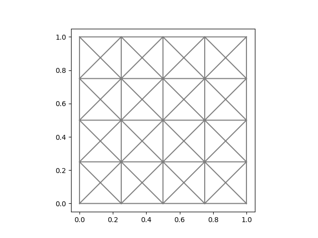
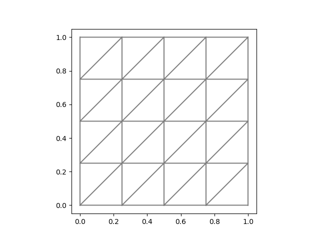
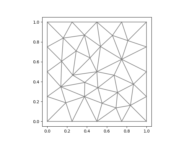
which corresponds to a Stokes problem, and homogeneous Dirichlet boundary conditions everywhere, that is $\Gamma_{N}=\emptyset$ (see, for instance, [11]). Since we also want to investigate the symmetry of the formulation, we consider three different mesh sequences: a symmetric and uniform mesh (CROSSED), a non-symmetric and uniform mesh (RIGHT), and a non structured non symmetric mesh (NONUNIF). The meshes are indexed with respect to the number $N$ of subdivisions of the square’s sides. The three meshes for $N=4$ are plotted in Figure 1.

In Table 1 we report the numerical results corresponding to computations performed with the two-field scheme (9) when using the three mesh sequences with the level of refinement varying from $N=4$ to $N=12$. We considered a second order scheme based on Raviart–Thomas elements for the approximation of $\Sigma_{h}$ (satisfying assumption (12)). The estimate of Theorem 3 predicts fourth order of convergence for the eigenvalues which is confirmed by our tests. It is interesting to observe that the fist computed eigenvalue is always real in our tests.

We performed the same computations for the three-field formulation presented in (10). Also in this case we use a second order scheme based on Raviart–Thomas elements (satisfying assumption (13)). The corresponding results are reported in Table 2. It turns out that also in this case the first computed eigenvalue is always real and that the convergence properties match the theoretical results with the exception of the convergence rate for $N=12$ on the non-uniform mesh. In order to check better this phenomenon, we computed one more refinement which is reported in Table 3. It is clear that the overall convergence matches the expected fourth order rate and that the non uniform behavior is due to the fact that the mesh sequence is not structured.

Since the eigenvalue problems corresponding to the considered formulations are not symmetric, it is interesting to investigate whether the computed eigenvalues are complex or real. From the results that we are going show, it is clear that in some cases the computed eigenvalues have a non-vanishing imaginary part; this implies that in general the discrete formulations cannot be reduced to symmetric problems. On the other hand, in most cases the computed eigenvalues are real; this occurs, in particular on the symmetric meshes.

In Table 4 we report the first five eigenvalues computed with the three-field scheme on the non-uniform mesh for $N=10$ (similar results could be presented for the two-field scheme as well). It is apparent that the second and the third eigenvalue are complex conjugate.

For the sake of comparison, Table 5 shows the same results on the mesh for $N=11$ and we can see that in this case all the first five eigenvalues are real. It is also interesting to observe that the second and the third eigenvalues on the mesh for $N=10$ have the same real part, while the corresponding eigenvalues on the mesh for $N=11$ are real and different from each other. Clearly they are an approximation of the double eigenvalue $\omega_{2}=\omega_{3}$. In any case, this is perfectly compatible with the statements of Theorems 3 and 4 where the difference $|\omega_{j}-\omega_{j,h}|$ has to be understood in the sense of the distance in the complex plane.

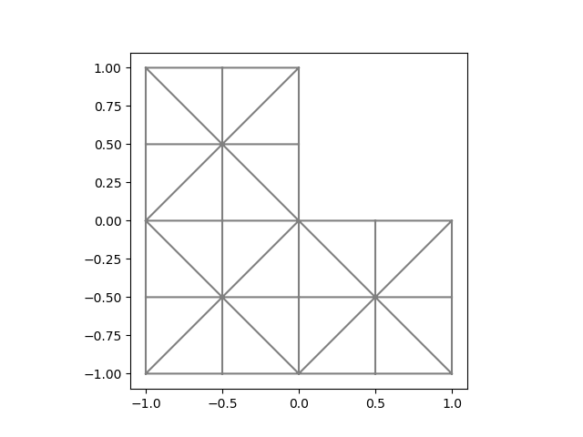
We conclude our numerical tests with computations on the L-shaped domain where the re-entrant corner causes singularities in the solution. We consider a uniform mesh (see Figure 2 for the case $N=4$).

An estimate of the first eigenvalues in this case has been provided in [5] and corresponds to $\omega=32.13269464746$. Tables 6 and 7 report on the computed approximation with the two- and three-field approximations (9) and (10), respectively. As expected, the singularity of the eigenfunction corresponding to the first eigenvalue causes a reduction of the order of convergence.

Also in this case the first computed eigenvalue is real, however, also in presence of a symmetric mesh, it turns out that there might be complex eigenvalues. For instance, Table 8 reports some higher eigenvalues computed for $N=8$. Also in this case the complex eigenvalues converge towards real number according to the statement of Theorems 3 and 4; moreover, the presence of complex eigenvalues depends on the mesh and on the level of refinements. The effect of the mesh on complex eigenvalues will be the object of further investigation.

References

- [1] Fenics project, https://fenicsproject.org/.
- [2] Douglas N. Arnold, Daniele Boffi, and Richard S. Falk, Quadrilateral finite elements, SIAM J. Numer. Anal. 42 (2005), no. 6, 2429–2451.
- [3] Ivo Babuška and John Osborn, Eigenvalue problems, Handbook of numerical analysis, Vol. II, Handb. Numer. Anal., II, North-Holland, Amsterdam, 1991, pp. 641–787.
- [4] Fleurianne Bertrand and Daniele Boffi, First order least-squares formulations for eigenvalue problems, arXiv:2002.08145 [math.NA], 2020.
- [5] Fleurianne Bertrand, Daniele Boffi, and Rui Ma, An adaptive finite element scheme for the Hellinger–Reissner elasticity mixed eigenvalue problem, submitted, 2020.
- [6] Fleurianne Bertrand, Zhiqiang Cai, and Eun Young Park, Least-squares methods for elasticity and Stokes equations with weakly imposed symmetry, Comput. Methods Appl. Math. 19 (2019), no. 3, 415–430.
- [7] Daniele Boffi, Finite element approximation of eigenvalue problems, Acta Numer. 19 (2010), 1–120.
- [8] Zhiqiang Cai and Jaeun Ku, The norm error estimates for the div least-squares method, SIAM J. Numer. Anal. 44 (2006), no. 4, 1721–1734.
- [9] Zhiqiang Cai and Gerhard Starke, Least-squares methods for linear elasticity, SIAM J. Numer. Anal. 42 (2004), no. 2, 826–842.
- [10] K. Andrew Cliffe, Tony J. Garratt, and Alastair Spence, Eigenvalues of block matrices arising from problems in fluid mechanics, SIAM J. Matrix Anal. Appl. 15 (1994), no. 4, 1310–1318.
- [11] Joscha Gedicke and Arbaz Khan, Arnold-Winther mixed finite elements for Stokes eigenvalue problems, SIAM J. Sci. Comput. 40 (2018), no. 5, A3449–A3469.
- [12] Vicente Hernandez, Jose E. Roman, and Vicente Vidal, SLEPc: A scalable and flexible toolkit for the solution of eigenvalue problems, ACM Trans. Math. Software 31 (2005), no. 3, 351–362.