Learning to Win Lottery Tickets in BERT Transfer via Task-agnostic Mask Training
Abstract
Recent studies on the lottery ticket hypothesis (LTH) show that pre-trained language models (PLMs) like BERT contain matching subnetworks that have similar transfer learning performance as the original PLM. These subnetworks are found using magnitude-based pruning. In this paper, we find that the BERT subnetworks have even more potential than these studies have shown. Firstly, we discover that the success of magnitude pruning can be attributed to the preserved pre-training performance, which correlates with the downstream transferability. Inspired by this, we propose to directly optimize the subnetwork structure towards the pre-training objectives, which can better preserve the pre-training performance. Specifically, we train binary masks over model weights on the pre-training tasks, with the aim of preserving the universal transferability of the subnetwork, which is agnostic to any specific downstream tasks. We then fine-tune the subnetworks on the GLUE benchmark and the SQuAD dataset. The results show that, compared with magnitude pruning, mask training can effectively find BERT subnetworks with improved overall performance on downstream tasks. Moreover, our method is also more efficient in searching subnetworks and more advantageous when fine-tuning within a certain range of data scarcity. Our code is available at https://github.com/llyx97/TAMT.
1 Introduction
The NLP community has witnessed a remarkable success of pre-trained language models (PLMs). After being pre-trained on unlabelled corpus in a self-supervised manner, PLMs like BERT Devlin et al. (2019) can be fine-tuned as a universal text encoder on a wide range of downstream tasks. However, the growing performance of BERT is driven, to a large extent, by scaling up the model size, which hinders the fine-tuning and deployment of BERT in resource-constrained scenarios.
At the same time, the lottery ticket hypothesis (LTH) Frankle and Carbin (2019) emerges as an active sub-field of model compression. The LTH states that randomly initialized dense networks contain sparse matching subnetworks, i.e., winning tickets (WTs), that can be trained in isolation to similar test accuracy as the full model. The original work of LTH and subsequent studies have demonstrated that such WTs do exist at random initialization or an early point of training Frankle et al. (2019, 2020). This implicates that it is possible to reduce training and inference cost via LTH.

Recently, Chen et al. (2020) extend the original LTH to the pre-training and fine-tuning paradigm, exploring the existence of matching subnetworks in pre-trained BERT. Such subnetworks are smaller in size, while they can preserve the universal transferability of the full model. Encouragingly, Chen et al. (2020) demonstrate that BERT indeed contains matching subnetworks that are transferable to multiple downstream tasks without compromising accuracy. These subnetworks are found using iterative magnitude pruning (IMP) Han et al. (2015) on the pre-training task of masked language modeling (MLM), or by directly compressing BERT with oneshot magnitude pruning (OMP), both of which are agnostic to any specific task.
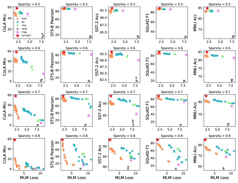
In this paper, we follow Chen et al. (2020) to study the question of LTH in BERT transfer learning. We find that there is a correlation, to certain extent, between the performance of a BERT subnetwork on the pre-training task (right after pruning), and its downstream performance (after fine-tuning). As shown by Fig. 1, the OMP subnetworks significantly outperform random subnetworks at 50% sparsity in terms of both MLM loss and downstream score. However, with the increase of model sparsity, the downstream performance and pre-training performance degrade simultaneously. This phenomenon suggests that we might be able to further improve the transferability of BERT subnetworks by discovering the structures that better preserve the pre-training performance.
To this end, we propose to search transferable BERT subnetworks via Task-Agnostic Mask Training (TAMT), which learns selective binary masks over the model weights on pre-training tasks. In this way, the structure of a subnetwork is directly optimized towards the pre-training objectives, which can preserve the pre-training performance better than heuristically retaining the weights with large magnitudes. The training objective of the masks is a free choice, which can be designed as any loss functions that are agnostic to the downstream tasks. In particular, we investigate the use of MLM loss and a loss based on knowledge distillation (KD) Hinton et al. (2015).
To examine the effectiveness of the proposal, we train the masks on the WikiText dataset Merity et al. (2017) for language modeling and then fine-tune the searched subnetworks on a wide variety of downstream tasks, including the GLUE benchmark Wang et al. (2019) for natural language understanding (NLU) and the SQuAD dataset Rajpurkar et al. (2016) for question answering (QA). The empirical results show that, through mask training, we can indeed find subnetworks with lower pre-training loss and better downstream transferability than OMP and IMP. Compared with IMP, which also involves training (the weights) on the pre-training task, mask training requires much fewer training iterations to reach the same performance. Moreover, the subnetworks found by mask training are generally more robust when being fine-tuned with reduced data, as long as the training data is not extremely scarce.
In summary, our contributions are:
-
•
We find that the pre-training performance of a BERT subnetwork correlates with its downstream transferability, which provides a useful insight for the design of methods to search transferable BERT subnetworks.
-
•
Based on the above finding, we propose to search subnetworks by learning binary masks over the weights of BERT, which can directly optimize the subnetwork structure towards the given pre-training objective.
-
•
Experiments on a variety of NLP tasks show that subnetworks found by mask training have better downstream performance than magnitude pruning. This suggests that BERT subnetworks have more potential, in terms of universal downstream transferability, than existing work has shown, which can facilitate our understanding and application of LTH on BERT.
2 Related Work
2.1 The Lottery Ticket Hypothesis
The lottery ticket hypothesis Frankle and Carbin (2019) suggests the existence of matching subnetworks, at random initialization, that can be trained in isolation to reach the performance of the original network. However, the matching subnetworks are found using IMP, which typically requires more training cost than the full network. There are two remedies to overcome this problem: Morcos et al. (2019) proposed to transfer the WT structure from source tasks to related target tasks, so that no further searching is required for the target tasks. You et al. (2020) draw early-bird tickets (prune the original network) at an early stage of training, and only train the subnetwork from then on.
Some recent works extend the LTH from random initialization to pre-trained initialization Prasanna et al. (2020); Chen et al. (2020); Liang et al. (2021); Chen et al. (2021b). Particularly, Chen et al. (2020) find that WTs, i.e., subnetworks of the pre-trained BERT, derived from the pre-training task of MLM using IMP are universally transferable to the downstream tasks. The same question of transferring WTs found in pre-training tasks is also explored in the CV field by Chen et al. (2021a); Caron et al. (2020). EarlyBERT Chen et al. (2021b) investigates drawing early-bird tickets of BERT. In this work, we follow the question of transferring WTs and seek to further improve the transferability of BERT subnetworks.
2.2 BERT Compression
In the literature of BERT compression, pruning LeCun et al. (1989); Han et al. (2015) and KD Hinton et al. (2015) are two widely-studied techniques. BERT can be pruned in either unstructured Gordon et al. (2020); Sanh et al. (2020); Mao et al. (2020) or structured Michel et al. (2019); Hou et al. (2020) ways. Although unstructured pruning is not hardware-friendly for speedup purpose, it is a common setup in LTH, and some recent efforts have been made in sparse tensor acceleration Elsen et al. (2020); Tambe et al. (2020). In BERT KD, various knowledge are explored, which includes the soft-labels Sanh et al. (2019), the hidden states Sun et al. (2019); Hou et al. (2020); Liu et al. (2021) and the attention relations Jiao et al. (2020), among others. Usually, pruning and KD are combined to compress the fine-tuned BERT. By contrast, the LTH compresses BERT before fine-tuning.
Another way to obtain more efficient BERT with the same transferability as the original one is to pre-train a compact model from scratch. This model can be trained either with the MLM objective Turc et al. (2019) or using pre-trained BERT as the teacher to perform KD Wang et al. (2020a); Sun et al. (2020); Jiao et al. (2020). By contrast, the LTH extracts subnetworks from BERT, which is about exposing the knowledge already learned by BERT, rather than learning new knowledge from scratch. Compared with training a new PLM, the LTH in BERT is still underexplored in the literature.
2.3 Learning Subnetwork Structure via Binary Mask Training
To make the subnetwork structure trainable, we need to back-propagate gradients through the binary masks. This can be achieved through the straight-through estimator Bengio et al. (2013) or drawing the mask variables from a hard-concrete distribution Louizos et al. (2018) and then using the re-parameterization trick. Mask training has been utilized in model compression Wang et al. (2020b); Sanh et al. (2020), and parameter-efficient training Mallya et al. (2018); Zhao et al. (2020); Radiya-Dixit and Wang (2020). However, unlike these works that learn the mask for each task separately (task-specific), we learn the subnetwork structure on pre-training task and transfer it to multiple downstream tasks (task-agnostic).

3 Methodology
3.1 BERT Architecture
BERT consists of an embedding layer and Transformer layers Vaswani et al. (2017). Each Transformer layer has two sub-layers: the self-attention layer and the feed-forward network (FFN).
The self-attention layer contains parallel attention heads and each head can be formulated as:
|
|
(1) |
where is the input; and are the hidden size and the length of input , respectively. are the query, key and value matrices, and . In practice, the matrices for different heads will be combined into three large matrices . The outputs of the heads are then concatenated and linearly projected by to obtain the final output of the self-attention layer.
The FFN consists of two weight matrices , with a GELU activation Hendrycks and Gimpel (2016) in between, where is the hidden dimension of FFN. Dropout Srivastava et al. (2014), residual connection He et al. (2016) and layer normalization Ba et al. (2016) are also applied following each sub-layer. Eventually, for each downstream task, a classifier is used to give the final prediction based on the output of the Transformer module.
3.2 Subnetwork and Magnitude Pruning
Consider a model with weights , we can obtain its subnetwork by applying a binary mask to , where denotes element-wise multiplication. In terms of BERT, we extract the subnetwork from the pre-trained weights . Specifically, we consider the matrices of the Transformer sub-layers and the word embedding matrix, i.e., .
Magnitude pruning Han et al. (2015) is initially used to compress a trained neural network by setting the low-magnitude weights to zero. It can be conducted in two different ways: 1) Oneshot magnitude pruning (OMP) directly prunes the trained weights to target sparsity while 2) iterative magnitude pruning (IMP) performs pruning and re-training iteratively until reaching the target sparsity. OMP and IMP are also widely studied in the literature of LTH as the method to find the matching subnetworks, with an additional operation of resetting the weights to initialization.
3.3 Problem Formulation: Transfer BERT Subnetwork
As depicted in Fig. 2, given downstream tasks , the subnetwork is fine-tuned on each task, together with the randomly initialized task-specific linear classifier . We formulate the training algorithm for task as a function (e.g., Adam or SGD), which trains the model for steps and produces . After fine-tuning, the model is evaluated against the metric (e.g., Accuracy or F1) for task .
In this work, we focus on finding a BERT subnetwork, that maximally preserves the overall downstream performance given a particular sparsity , especially at the sparsity that magnitude pruning performs poorly. This can be formalized as:
| (2) |
where and are the norm of the mask and the total number of model weights respectively.
3.4 Task-agnostic Mask Training
3.4.1 Mask Training with Binarization and Gradient Estimation
In order to learn the binary masks, we adopt the technique for training binarized neural networks Hubara et al. (2016), following Zhao et al. (2020); Mallya et al. (2018). This technique involves mask binarization in the forward pass and gradient estimation in the backward pass.
As shown in Fig. 2, each weight matrix is associated with a binary mask , which is derived from a real-valued matrix via binarization:
| (3) |
where is the threshold that controls the sparsity. In the forward pass of a subnetwork, is used in replacement of the original weights .
Since are discrete variables, the gradient signals cannot be back-propagated through the binary mask. We therefore use the straight-through estimator Bengio et al. (2013) to approximate the gradients and update the real-valued mask:
| (4) |
where is the loss function and is the learning rate. In other words, the gradients of is estimated using the gradients of . In the process of mask training, all the original weights are frozen.
3.4.2 Mask Initialization and Sparsity Control
The real-valued masks can be initialized in various forms, e.g., random initialization. Considering that magnitude pruning can preserve the pre-training knowledge to some extent, and OMP is easy to implement with almost zero computation cost, we directly initialize using OMP:
| (5) |
where is the binary mask derived from OMP and is a hyper-parameter. In this way, the weights with large magnitudes will be retained at initialization according to Eq. 3, because the corresponding . In practice, we perform OMP over the weights locally based on the given sparsity, which means the magnitudes are ranked inside each weight matrix.
As being updated, some of its entries with zero initialization will gradually surpass the threshold, and vice versa. If the threshold is fixed throughout training, there is no guarantee that the binary mask will always satisfy the given sparsity. Therefore, we rank according to their absolute values during mask training, and dynamically adjust the threshold to satisfy the sparsity constraint.
3.4.3 Mask Training Objectives
We explore the use of two objectives for mask training, namely the MLM loss and the KD loss.
The MLM is the original task used in BERT pre-training. It randomly replaces a portion of the input tokens with the token, and requires the model to reconstruct the original tokens based on the entire masked sequence. Concretely, the MLM objective is computed as cross-entropy loss on the predicted masked tokens. During MLM learning, we allow the token classifier (i.e., the in Fig. 2) to be trainable, in addition to the masks.
In KD, the compressed model (student) is trained with supervision from the original model (teacher). Under our framework of mask training, the training signal can also be derived from the unpruned BERT. To this end, we design the KD objective by encouraging the subnetwork to mimic the representations of the original BERT, which is shown to be a useful source of knowledge in BERT KD Sun et al. (2019); Hou et al. (2020). Specifically, the distillation loss is formulated as the cosine similarity between the teacher’s and student’s representations:
| (6) |
where is the hidden state of the token at the layer; and denote the teacher and student respectively; is the cosine similarity.
4 Experiments
4.1 Experimental Setups
4.1.1 Models
We examine two PLMs from the BERT family, i.e., Devlin et al. (2019) and Liu et al. (2019). They have basically the same structure, while differ in the vocabulary size, which results in approximately 110M and 125M parameters respectively. The main results of Section 4.2.1 study both two models. For the analytical studies, we only use .


4.1.2 Baselines, Datasets and Evaluation
We compare our mask training method with IMP, OMP as well as subnetworks with random structures. Following Chen et al. (2020), we use the MLM loss during IMP training. For TAMT, we consider three variants, namely TAMT-MLM that uses MLM as training objective, TAMT-KD that uses the KD objective (Eq. 6), and TAMT-MLM+KD that equally combines MLM and KD.
We build our pre-training set using the WikiText-103 dataset Merity et al. (2017) for language modeling. For downstream fine-tuning, we use six datasets, i.e., CoLA, SST-2, RTE, MNLI, MRPC and STS-B from the GLUE benchmark for NLU and the SQuAD v1.1 dataset for QA.
Evaluations are conducted on the dev sets. For the downstream tasks, we follow the standard evaluation metrics Wang et al. (2019). For the pre-training tasks, we calculate the MLM and KD loss on the dev set of WikiText-103. More information about the datasets and evaluation metrics can be found in Appendix B.1.
4.1.3 Implementation Details
Both TAMT and IMP are conducted on the pre-training dataset. For mask training, we initialize the mask using OMP as described in Section 3.4.2. We also provide a comparison between OMP and random initialization in Section 4.2.4. The initial threshold and are set to and 2 respectively, which work well in our experiments. For IMP, we increase the sparsity by every 1/10 of total training iterations, until reaching the target sparsity, following Chen et al. (2020). Every pruning operation in IMP is followed by resetting the remaining weights to . In the fine-tuning stage, all the models are trained using the same set of hyper-parameters unless otherwise specified.
For TAMT, IMP and random pruning, we generate three subnetworks with different seeds, and the result of each subnetwork is also averaged across three runs, i.e., the result of every method is the average of nine runs in total. For OMP, we can only generate one subnetwork, which is fine-tuned across three runs. More implementation details and computing budgets can be found in Appendix B.2.

4.2 Results and Analysis
4.2.1 Main Results
Fig. 3 and Fig. 4 present the downstream performance of BERT and RoBERTa subnetworks, respectively. We can derive the following observations:
There is a clear gap between random subnetworks and the other ones found with certain inductive bias. At sparsity for BERT and for RoBERTa, all the methods, except for “Rand”, maintain of the full model’s overall performance. As sparsity grows, the OMP subnetworks degrade significantly. IMP, which is also based on magnitude, exhibits relatively mild declines.
TAMT further outperforms IMP with perceivable margin. For BERT subnetworks, the performance of TAMT variants are close to each other, which have advantage over IMP across sparsity. When it comes to RoBERTa, the performance of TAMT-KD is undesirable at sparsity, which only slightly outperforms IMP. In comparison, TAMT-MLM consistently surpasses IMP and TAMT-KD on RoBERTa.
Combining MLM and KD leads to comparable average performance as TAMT-MLM for BERT, while slightly improves over TAMT-MLM for RoBERTa. This suggests that the two training objectives could potentially benefit, or at least will not negatively impact each other. In Section 4.2.2, we will show that the MLM and KD objectives indeed exhibit certain consistency.
At sparsity, all the methods perform poorly, with average scores approximately half of the full model. On certain tasks like CoLA, RTE and MRPC, drastic performance drop of all methods can even be observed at lower sparsity (e.g., ). This is probably because the number of training data is too scarce in these tasks for sparse PLMs to perform well. However, we find that the advantage of TAMT is more significant within a range of data scarsity, which will be discussed in Section 4.2.6.
We also note that RoBERTa, although outperforms BERT as a full model, is more sensitive to task-agnostic pruning. A direct comparison between the two PLMs is provided in Appendix A.2.
4.2.2 The Effect of Pre-training Performance
As we discussed in Section 1, our motivation of mask training is to improve downstream transferability by preserving the pre-training performance. To examine whether the effectiveness of TAMT is indeed derived from the improvement on pre-training tasks, we calculate the MLM/KD dev loss for the subnetworks obtained from the mask training process, and associate it with the downstream performance. The results are shown in Fig. 5, where the "Avg Score" includes CoLA, SST-2, MNLI, STS-B and SQuAD. In the following sections, we also mainly focus on these five tasks. We can see from Fig. 5 that:
There is a positive correlation between the pre-training and downstream performance, and this trend can be observed for subnetworks across different sparsities. Compared with random pruning, the magnitude pruning subnetworks and TAMT subnetworks reside in an area with lower MLM/KD loss and higher downstream score at sparsity. As sparsity increases, OMP subnetworks gradually move from the upper-left to the lower-right area of the plots. In comparison, IMP is better at preserving the pre-training performance, even though it is not deliberately designed for this purpose. For this reason, hypothetically, the downstream performance of IMP is also better than OMP.
TAMT-MLM and TAMT-KD have the lowest MLM and KD loss respectively, which demonstrates that the masks are successfully optimized towards the given objectives. As a result, the downstream performance is also elevated from the OMP initialization, which justifies our motivation. Moreover, training the mask with KD loss can also optimize the performance on MLM, and vice versa, suggesting that there exists some consistency between the objectives of MLM and KD.
It is also worth noting that the correlation between pre-training and fine-tuning performance is not ubiquitous. For example, among the subnetworks of OMP, IMP and TAMT at sparsity, the decrease in KD/MLM loss produces little or no downstream improvement; at sparsity, OMP underperforms random pruning in MLM, while its downstream performance is better. These phenomenons suggest that some properties about the BERT winning tickets are still not well-understood by us.


4.2.3 The Effect of Pre-training Cost
We have shown that mask training is more effective than magnitude pruning. Now let us take a closer look at the results of TAMT and IMP with different iterations of pre-training, to evaluate their efficiency in subnetwork searching. For TAMT, we directly obtain the subnetworks from varied pre-training iterations. For IMP, we change the pruning frequency to control the number of training iterations before reaching the target sparsity.
Fig. 6 presents the downstream results with increased pre-training iterations and time. We can see that for all the methods, the fine-tuning performance steadily improves as pre-training proceeds. Along this process, TAMT advances at a faster pace, reaching the best score achieved by IMP with fewer iterations and fewer time. This indicates that directly optimizing the pre-training objectives is more efficient than the iterative process of weight pruning and re-training.
4.2.4 The Effect of Mask Initialization
In the main results, we use OMP as the default initialization, in order to provide a better start point for TAMT. To validate the efficacy of this setting, we compare OMP initialization with random initialization. Concretely, we randomly sample some entries of the real-valued masks to be zero, according to the given sparsity, and use the same and for the non-zero entries as in Eq. 5.
The results are shown in Fig. 7. We can see that, for random initialization, TAMT can still steadily improve the downstream performance as pre-training proceeds. However, the final results of TAMT-MLM/KD (Rand_init) are significantly worse than TAMT-MLM/KD, which demonstrates the necessity of using OMP as initialization.
4.2.5 Similarity between Subnetworks
The above results show that the subnetworks found by different methods perform differently. We are therefore interested to see how they differ in the mask structure. To this end, we compute the similarity between OMP mask and the masks derived during the training of TAMT and IMP. Following Chen et al. (2020), we measure the Jaccard similarity between two binary masks and as , and the mask distance is defined as .
From the results of Fig. 8, we can find that: 1) With different objectives, TAMT produces different mask structures. The KD loss results in masks in the close proximity of OMP initialization, while the MLM masks deviate away from OMP. 2) Among the four methods, IMP and TAMT-MLM have the highest degree of dissimilarity, despite the fact that they both involve MLM training. 3) Although IMP, TAMT-KD and TAMT-MLM are different from each other in terms of subnetwork structure, all of them clearly improves over the OMP baseline. Therefore, we hyphothesize that the high-dimensional binary space might contain multiple regions of winning tickets that are disjoint with each other. Searching methods with different inductive biases (e.g., mask training versus pruning and KD loss versus MLM loss) are inclined to find different regions of interest.

4.2.6 Results of Reducing Fine-tuning Data
To test the fine-tuning results with reduced data, we select four tasks (CoLA, SST-2, MNLI and SQuAD) with the largest data sizes and shrink them from the entire training set to 1,000 samples.
Fig. 9 summarizes the results of subnetworks found using different methods, as well as results of full BERT as a reference. We can see that the four datasets present different patterns. For MNLI and SQuAD, the advantage of TAMT first increases and then decreases with the reduction of data size. The turning point appears at around 10,000 samples, after which the performance of all methods, including the full BERT, degrade drastically (note that the horizontal axis is in log scale). For SST-2, the performance gap is enlarged continuously until we have only 1,000 data. With regard to CoLA, the gap between TAMT and IMP shrinks as we reduce the data size, which is not desirable. However, a decrease in the gap between full BERT and IMP is also witnessed when the data size is reduced under 5,000 samples. This is in part because the Mcc of IMP is already quite low even with the entire training set, and thus the performance decrease of IMP is limited compared with TAMT. However, the results on CoLA, as well as the results on MNLI and SQuAD with less than 10,000 samples, also suggest an inherent difficulty of learning with limited data for subnetworks at high sparsity, which is also discussed in the main results.
5 Conclusions
In this paper, we address the problem of searching transferable BERT subnetworks. We first show that there exist correlations between the pre-training performance and downstream transferablility of a subnetwork. Motivated by this, we devise a subnetwork searching method based on task-agnostic mask training (TAMT). We empirically show that TAMT with MLM loss or KD loss achieve better pre-training and downstream performance than the magnitude pruning, which is recently shown to be successful in finding universal BERT subnetworks. TAMT is also more efficient in mask searching and produces more robust subnetworks when being fine-tuned within a certain range of data scarsity.
6 Limitations and Future Work
Under the framework of TAMT, there are still some unsolved challenges and interesting questions worth studying in the future work: First, we focus on unstructured sparsity in this work, which is hardware-unfriendly for speedup purpose. In future work, we are interested in investigating TAMT with structured pruning or applying unstructured BERT subnetworks on hardware platforms that support sparse tensor acceleration Elsen et al. (2020); Tambe et al. (2020). Second, despite the overall improvement achieved by TAMT, it fails at extreme sparsity or when the labeled data for a task is too scarce. Therefore, another future direction is to further promote the performance of universal PLM subnetworks on these challenging circumstances. To achieve this goal, thirdly, a feasible way is to explore other task-agnostic training objectives for TAMT beyond MLM and hidden state KD, e.g., self-attention KD Jiao et al. (2020) and contrastive learning Gao et al. (2021). An in-depth study on the selection of TAMT training objective might further advance our understanding of TAMT and the LTH of BERT.
Acknowledgments
This work was supported by the National Natural Science Foundation of China under Grants 61976207 and 61906187.
References
- Ba et al. (2016) Lei Jimmy Ba, Jamie Ryan Kiros, and Geoffrey E. Hinton. 2016. Layer normalization. CoRR, abs/1607.06450.
- Bengio et al. (2013) Yoshua Bengio, Nicholas Léonard, and Aaron C. Courville. 2013. Estimating or propagating gradients through stochastic neurons for conditional computation. CoRR, abs/1308.3432.
- Caron et al. (2020) Mathilde Caron, Ari Morcos, Piotr Bojanowski, Julien Mairal, and Armand Joulin. 2020. Pruning convolutional neural networks with self-supervision. CoRR, abs/2001.03554.
- Chen et al. (2021a) Tianlong Chen, Jonathan Frankle, Shiyu Chang, Sijia Liu, Yang Zhang, Michael Carbin, and Zhangyang Wang. 2021a. The lottery tickets hypothesis for supervised and self-supervised pre-training in computer vision models. In CVPR, pages 16306–16316.
- Chen et al. (2020) Tianlong Chen, Jonathan Frankle, Shiyu Chang, Sijia Liu, Yang Zhang, Zhangyang Wang, and Michael Carbin. 2020. The lottery ticket hypothesis for pre-trained BERT networks. In NeurIPS, pages 15834–15846.
- Chen et al. (2021b) Xiaohan Chen, Yu Cheng, Shuohang Wang, Zhe Gan, Zhangyang Wang, and Jingjing Liu. 2021b. Earlybert: Efficient BERT training via early-bird lottery tickets. In ACL/IJCNLP, pages 2195–2207. Association for Computational Linguistics.
- Devlin et al. (2019) Jacob Devlin, Ming-Wei Chang, Kenton Lee, and Kristina Toutanova. 2019. BERT: pre-training of deep bidirectional transformers for language understanding. In NAACL-HLT, pages 4171–4186.
- Elsen et al. (2020) Erich Elsen, Marat Dukhan, Trevor Gale, and Karen Simonyan. 2020. Fast sparse convnets. In CVPR, pages 14617–14626. Computer Vision Foundation / IEEE.
- Frankle and Carbin (2019) Jonathan Frankle and Michael Carbin. 2019. The lottery ticket hypothesis: Finding sparse, trainable neural networks. In ICLR. OpenReview.net.
- Frankle et al. (2019) Jonathan Frankle, Gintare Karolina Dziugaite, Daniel M. Roy, and Michael Carbin. 2019. The lottery ticket hypothesis at scale. CoRR, abs/1903.01611.
- Frankle et al. (2020) Jonathan Frankle, Gintare Karolina Dziugaite, Daniel M. Roy, and Michael Carbin. 2020. Linear mode connectivity and the lottery ticket hypothesis. In ICML, volume 119 of Proceedings of Machine Learning Research, pages 3259–3269. PMLR.
- Gao et al. (2021) Tianyu Gao, Xingcheng Yao, and Danqi Chen. 2021. Simcse: Simple contrastive learning of sentence embeddings. In EMNLP, pages 6894–6910. Association for Computational Linguistics.
- Gordon et al. (2020) Mitchell A. Gordon, Kevin Duh, and Nicholas Andrews. 2020. Compressing BERT: studying the effects of weight pruning on transfer learning. In RepL4NLP@ACL, pages 143–155.
- Han et al. (2015) Song Han, Jeff Pool, John Tran, and William Dally. 2015. Learning both weights and connections for efficient neural network. In Advances in Neural Information Processing Systems 28, pages 1135–1143. Curran Associates, Inc.
- He et al. (2016) Kaiming He, Xiangyu Zhang, Shaoqing Ren, and Jian Sun. 2016. Deep residual learning for image recognition. In CVPR, pages 770–778. IEEE Computer Society.
- Hendrycks and Gimpel (2016) Dan Hendrycks and Kevin Gimpel. 2016. Bridging nonlinearities and stochastic regularizers with gaussian error linear units. CoRR, abs/1606.08415.
- Hinton et al. (2015) Geoffrey E. Hinton, Oriol Vinyals, and Jeffrey Dean. 2015. Distilling the knowledge in a neural network. CoRR, abs/1503.02531.
- Hou et al. (2020) Lu Hou, Zhiqi Huang, Lifeng Shang, Xin Jiang, Xiao Chen, and Qun Liu. 2020. Dynabert: Dynamic BERT with adaptive width and depth. In NeurIPS, pages 9782–9793.
- Hubara et al. (2016) Itay Hubara, Matthieu Courbariaux, Daniel Soudry, Ran El-Yaniv, and Yoshua Bengio. 2016. Binarized neural networks. In NIPS, pages 4107–4115.
- Jiao et al. (2020) Xiaoqi Jiao, Yichun Yin, Lifeng Shang, Xin Jiang, Xiao Chen, Linlin Li, Fang Wang, and Qun Liu. 2020. Tinybert: Distilling BERT for natural language understanding. In EMNLP (Findings), pages 4163–4174.
- LeCun et al. (1989) Yann LeCun, John S. Denker, and Sara A. Solla. 1989. Optimal brain damage. In NIPS, pages 598–605. Morgan Kaufmann.
- Liang et al. (2021) Chen Liang, Simiao Zuo, Minshuo Chen, Haoming Jiang, Xiaodong Liu, Pengcheng He, Tuo Zhao, and Weizhu Chen. 2021. Super tickets in pre-trained language models: From model compression to improving generalization. In ACL/IJCNLP, pages 6524–6538. Association for Computational Linguistics.
- Liu et al. (2019) Yinhan Liu, Myle Ott, Naman Goyal, Jingfei Du, Mandar Joshi, Danqi Chen, Omer Levy, Mike Lewis, Luke Zettlemoyer, and Veselin Stoyanov. 2019. Roberta: A robustly optimized BERT pretraining approach. CoRR, abs/1907.11692.
- Liu et al. (2021) Yuanxin Liu, Fandong Meng, Zheng Lin, Weiping Wang, and Jie Zhou. 2021. Marginal utility diminishes: Exploring the minimum knowledge for BERT knowledge distillation. In ACL/IJCNLP, pages 2928–2941.
- Loshchilov and Hutter (2019) Ilya Loshchilov and Frank Hutter. 2019. Decoupled weight decay regularization. In ICLR (Poster). OpenReview.net.
- Louizos et al. (2018) Christos Louizos, Max Welling, and Diederik P. Kingma. 2018. Learning sparse neural networks through l_0 regularization. In ICLR (Poster). OpenReview.net.
- Mallya et al. (2018) Arun Mallya, Dillon Davis, and Svetlana Lazebnik. 2018. Piggyback: Adapting a single network to multiple tasks by learning to mask weights. In ECCV (4), volume 11208 of Lecture Notes in Computer Science, pages 72–88. Springer.
- Mao et al. (2020) Yihuan Mao, Yujing Wang, Chufan Wu, Chen Zhang, Yang Wang, Quanlu Zhang, Yaming Yang, Yunhai Tong, and Jing Bai. 2020. Ladabert: Lightweight adaptation of BERT through hybrid model compression. In COLING, pages 3225–3234.
- Merity et al. (2017) Stephen Merity, Caiming Xiong, James Bradbury, and Richard Socher. 2017. Pointer sentinel mixture models. In ICLR (Poster). OpenReview.net.
- Michel et al. (2019) Paul Michel, Omer Levy, and Graham Neubig. 2019. Are sixteen heads really better than one? In NeurIPS, pages 14014–14024.
- Morcos et al. (2019) Ari S. Morcos, Haonan Yu, Michela Paganini, and Yuandong Tian. 2019. One ticket to win them all: generalizing lottery ticket initializations across datasets and optimizers. In NeurIPS, pages 4933–4943.
- Prasanna et al. (2020) Sai Prasanna, Anna Rogers, and Anna Rumshisky. 2020. When BERT plays the lottery, all tickets are winning. In EMNLP, pages 3208–3229.
- Radiya-Dixit and Wang (2020) Evani Radiya-Dixit and Xin Wang. 2020. How fine can fine-tuning be? learning efficient language models. In AISTATS, volume 108 of Proceedings of Machine Learning Research, pages 2435–2443. PMLR.
- Rajpurkar et al. (2016) Pranav Rajpurkar, Jian Zhang, Konstantin Lopyrev, and Percy Liang. 2016. Squad: 100, 000+ questions for machine comprehension of text. In EMNLP, pages 2383–2392.
- Sanh et al. (2019) Victor Sanh, Lysandre Debut, Julien Chaumond, and Thomas Wolf. 2019. Distilbert, a distilled version of BERT: smaller, faster, cheaper and lighter. CoRR, abs/1910.01108.
- Sanh et al. (2020) Victor Sanh, Thomas Wolf, and Alexander M. Rush. 2020. Movement pruning: Adaptive sparsity by fine-tuning. In NeurIPS, pages 20378–20389.
- Srivastava et al. (2014) Nitish Srivastava, Geoffrey E. Hinton, Alex Krizhevsky, Ilya Sutskever, and Ruslan Salakhutdinov. 2014. Dropout: a simple way to prevent neural networks from overfitting. J. Mach. Learn. Res., 15(1):1929–1958.
- Sun et al. (2019) Siqi Sun, Yu Cheng, Zhe Gan, and Jingjing Liu. 2019. Patient knowledge distillation for BERT model compression. In EMNLP/IJCNLP, pages 4322–4331.
- Sun et al. (2020) Zhiqing Sun, Hongkun Yu, Xiaodan Song, Renjie Liu, Yiming Yang, and Denny Zhou. 2020. Mobilebert: a compact task-agnostic BERT for resource-limited devices. In ACL, pages 2158–2170. Association for Computational Linguistics.
- Tambe et al. (2020) Thierry Tambe, Coleman Hooper, Lillian Pentecost, En-Yu Yang, Marco Donato, Victor Sanh, Alexander M. Rush, David Brooks, and Gu-Yeon Wei. 2020. Edgebert: Optimizing on-chip inference for multi-task NLP. CoRR, abs/2011.14203.
- Turc et al. (2019) Iulia Turc, Ming-Wei Chang, Kenton Lee, and Kristina Toutanova. 2019. Well-read students learn better: The impact of student initialization on knowledge distillation. CoRR, abs/1908.08962.
- Vaswani et al. (2017) Ashish Vaswani, Noam Shazeer, Niki Parmar, Jakob Uszkoreit, Llion Jones, Aidan N. Gomez, Lukasz Kaiser, and Illia Polosukhin. 2017. Attention is all you need. In NIPS, pages 5998–6008.
- Wang et al. (2019) Alex Wang, Amanpreet Singh, Julian Michael, Felix Hill, Omer Levy, and Samuel R. Bowman. 2019. GLUE: A multi-task benchmark and analysis platform for natural language understanding. In ICLR (Poster). OpenReview.net.
- Wang et al. (2020a) Wenhui Wang, Furu Wei, Li Dong, Hangbo Bao, Nan Yang, and Ming Zhou. 2020a. Minilm: Deep self-attention distillation for task-agnostic compression of pre-trained transformers. In NeurIPS, pages 5776–5788.
- Wang et al. (2020b) Ziheng Wang, Jeremy Wohlwend, and Tao Lei. 2020b. Structured pruning of large language models. In EMNLP, pages 6151–6162. Association for Computational Linguistics.
- Wolf et al. (2020) Thomas Wolf, Lysandre Debut, Victor Sanh, Julien Chaumond, Clement Delangue, Anthony Moi, Pierric Cistac, Tim Rault, Rémi Louf, Morgan Funtowicz, Joe Davison, Sam Shleifer, Patrick von Platen, Clara Ma, Yacine Jernite, Julien Plu, Canwen Xu, Teven Le Scao, Sylvain Gugger, Mariama Drame, Quentin Lhoest, and Alexander M. Rush. 2020. Transformers: State-of-the-art natural language processing. In Proceedings of the 2020 Conference on Empirical Methods in Natural Language Processing: System Demonstrations, pages 38–45, Online.
- You et al. (2020) Haoran You, Chaojian Li, Pengfei Xu, Yonggan Fu, Yue Wang, Xiaohan Chen, Richard G. Baraniuk, Zhangyang Wang, and Yingyan Lin. 2020. Drawing early-bird tickets: Toward more efficient training of deep networks. In ICLR. OpenReview.net.
- Zhao et al. (2020) Mengjie Zhao, Tao Lin, Fei Mi, Martin Jaggi, and Hinrich Schütze. 2020. Masking as an efficient alternative to finetuning for pretrained language models. In EMNLP, pages 2226–2241.

Appendix A More Results and Analysis
A.1 Single Task Downstream Performance of OMP and Random Pruning
In Fig. 1 of the main body of paper, we show that the pre-training and overall downstream performance of OMP, as well as the gap between “OMP" and “Rand", degrade simultaneously as sparsity increases. The detailed results of each downstream task are presented in Fig. 10. As we can see, the general pattern for every task is similar, with the exception that the gap between “OMP" and “Rand" slightly increases before high sparsity on tasks RTE, MNLI and SQuAD.
Pre-training Fine-tuning IMP-MLM TAMT-MLM TAMT-KD TAMT-MLM+KD MNLI SST-2 CoLA STS-B MRPC RTE SQuAD # Train Samples 103M 103M 103M 103M 392K 67K 8.5K 5.7K 3.6K 2.4K 88K # Eval Samples 217K 217K 217K 217K 9.8K 0.8K 1K 1.5K 0.4K 0.2K 10K Max Epochs 2 - - - 3 3 3 3 3 3 2 Eval Iter - - - - 500 50 50 50 50 50 1K Batch Size 16 16 16 16 32 32 32 32 32 32 16 Max Length 512 512 512 512 128 128 128 128 128 128 384 Lr (linear decay) 5e-5 5e-5 2e-5 5e-5 2e-5 2e-5 2e-5 2e-5 2e-5 2e-5 3e-5 Eval Metric Dev Loss Dev Loss Dev Loss - Matched Acc Acc Matthew’s Corr Pearson Corr Acc Acc F1 Optimizer AdamW Loshchilov and Hutter (2019)
20% 30% 40% 50% 60% 70% 80% 90% IMP 2.79K 5.58K 8.38K 11.17K 13.96K 16.75K 19.54K 22.34K TAMT 3K 6K 8K 11K 14K 17K 20K 22K
IMP TAMT-MLM TAMT-KD 4h6m26s 3h54m58s 4h46m46s 4h33m9s 4h17m15s 4h51m55s
A.2 Comparison Between BERT and RoBERTa Subnetworks
In the main results of Fig. 3 and Fig. 4, we compare the fine-tuning performance of subnetworks of the same PLM but found using different methods. In this section, we give a comparison between subnetwords of and . As shown in Fig. 11, RoBERTa consistently outperforms BERT as a full model. However, as we prune the pre-trained weights accroding to the magnitudes, the performance of RoBERTa declines more sharply than BERT, leading to worse results of RoBERTa subnetworks when crossing a certain sparsity threshold. This phenomenon suggests that, compared with BERT, RoBERTa is less robust to task-agnostic magnitude pruning. More empirical and theoretical analysis are required to understand the underlying reasons.
A.3 Pre-training Performance and Single Task Downstream Performance
The relation between pre-training performance and overall downstream performance is illustrated in Fig. 5. Here in this appendix, we provide the detailed results about each single downstream task, as shown in Fig. 12 and Fig. 13. As we can see, the pattern in each single task is general the same as we discussed in Section 4.2.2. When the model sparsity is higher than , TAMT promotes the performance of OMP in terms of both pre-training tasks and downstream tasks, and improves over IMP with perceivable margin. As shown in Fig. 3 and Fig. 4 of the main paper, both IMP and TAMT display no obvious improvement over OMP on MRPC and RTE (but no degradation as well). Therefore, we do not report the comparison on these two datasets.
A.4 Pre-training Iteration and Single Task Downstream Performance
In Fig. 6, we show the overall downstream performance at sparsity with the increase of mask training iterations. Here, we report the results of each single downstream task from sparsities, which are shown in Fig. 14, Fig. 15 and Fig. 16. We can see that: 1) The single task performance of both TAMT-MLM and TAMT-KD grows faster than IMP at and sparsity, with the only exception of STS-B, where TAMT-MLM and IMP are comparable in the early stage of pre-training. 2) The MLM and KD objectives are good at different sparsity levels and different tasks. TAMT-KD performs the best at sparsity, surpassing TAMT-MLM on all the five tasks. In contrast, TAMT-MLM is better at higher sparsities. 3) At sparsity, the searching efficiency of the KD objective is not desirable, which requires more pre-training steps to outperform IMP on CoLA, STS-B, SQuAD and the overall performance. However, the advantage of TAMT-MLM is still obvious at sparsity.
A.5 Subnetwork Similarity at Different Sparsities
In Section 4.2.5, we analyse the similarity between subnetworks at sparsity. In Fig. 17, we present additional results of subnetworks at different sparsities. We can see that the general pattern, as discussed in Section 4.2.5, is the same across , and sparsities. However, as sparsity grows, different searching methods becomes more distinct from each other. For instance, the similarity between TAMT-MLM and IMP subnetworks decreases from 0.75 at sparsity to less than 0.6 at sparsity. This is understandable because the higher the sparsity, the lower the probability that two subnetworks will share the same weight.
Appendix B More Information about Experimental Setups
B.1 Datasets and Evaluation
For pre-training, we adopt the WikiText-103 dataset 111WikiText-103 is available under the Creative Commons Attribution-ShareAlike License (https://en.wikipedia.org/wiki/Wikipedia:Text_of_Creative_Commons_Attribution-ShareAlike_3.0_Unported_License) for language modeling. WikiText-103 is a collection of articles on Wikipedia and has over 100M tokens. Such data scale is relatively small for PLM pre-training. However, we find that it is sufficient for mask training and IMP to discover subnetworks with perceivable downstream improvement.
For the downstream tasks, we use six datasets from the GLUE benchmark and the SQuAD v1.1 dataset 222SQuAD is available under the CC BY-SA 4.0 license.. The GLUE benchmark is intended to train, evaluate, and analyze NLU systems. Our experiments include the tasks of CoLA for linguistic acceptability, SST-2 for sentiment analysis, RTE and MNLI for natural language inference, MRPC and STS-B for semantic matching/similarity. The SQuAD dataset is for the task of question answering. It consists of questions posed by crowdworkers on a set of Wikipedia articles. Tab. 1 summarizes the dataset statistics and evaluation metrics. All the datasets are in English language.
B.2 Implementation Details
The hyper-parameters for pre-training and fine-tuning are shown in Tab. 1. The pre-training setups of IMP basically follow Chen et al. (2020), except for the number of training epochs, because we use different pre-training datasets. Since we aim at finding universal PLM subnetworks that are agnostic to the downstream tasks, we do not perform hyper-parameter search for TAMT based on the downstream performance. The pre-training hyper-parameters in Tab. 1 are determined as they can guarantee stable convergence on the pre-training tasks.
For fair comparison between TAMT and IMP, we control the number of pre-training iterations (i.e., the number of gradient descent steps) to be the same. Considering that the IMP subnetworks of different sparsities are obtained from different pre-training iterations, we adjust the pre-training iterations of TAMT accordingly. Specifically, we set the maximum number of pre-training epochs to 2 for IMP, which equals to 27.92K training iterations. Thus, the sparsity is increased by 10% every 2.792K iterations. Tab. 2 shows the number of pre-training iterations for IMP and TAMT subnetworks at sparsity. Note that the final training iteration does not equal to 27.92K at sparsity according to Tab. 2. This is because we prune to sparsity at the iteration, which follows the implementation of Chen et al. (2020).
The hyper-parameters for downstream fine-tuning follow the standard setups of Wolf et al. (2020); Chen et al. (2020). We use the same set of hyper-parameters for all the subnetworks, as well as the full models. We perform evaluations during the fine-tuning process, and the best result is reported as the downstream performance.
Training and evaluation are implemented on Nvidia V100 GPU. The codes are based on the Pytorch framework333https://pytorch.org/ and the huggingface Transformers library444https://github.com/huggingface/transformers Wolf et al. (2020). Tab. 3 shows the pre-training time of IMP and TAMT.