Learning to Localize Using a LiDAR Intensity Map
Abstract
In this paper we propose a real-time, calibration-agnostic and effective localization system for self-driving cars. Our method learns to embed the online LiDAR sweeps and intensity map into a joint deep embedding space. Localization is then conducted through an efficient convolutional matching between the embeddings. Our full system can operate in real-time at 15Hz while achieving centimeter level accuracy across different LiDAR sensors and environments. Our experiments illustrate the performance of the proposed approach over a large-scale dataset consisting of over 4000km of driving.
Keywords: Deep Learning, Localization, Map-based Localization
1 Introduction
One of the fundamental problems in autonomous driving is to be able to accurately localize the vehicle in real time. Different precision requirements exist depending on the intended use of the localization system. For routing the self-driving vehicle from point A to point B, precision of a few meters is sufficient. However, centimeter-level localization becomes necessary in order to exploit high definition (HD) maps as priors for robust perception, prediction, and safe motion planning.
Despite many decades of research, reliable and accurate localization remains an open problem, especially when very low latency is required. Geometric methods, such as those based on the iterative closest-point algorithm (ICP) [1, 2] can lead to high-precision localization, but remain vulnerable in the presence of geometrically non-distinctive or repetitive environments, such as tunnels, highways, or bridges. Image-based methods [3, 4, 5, 6] are also capable of robust localization, but are still behind geometric ones in terms of outdoor localization precision. Furthermore, they often require capturing the environment in different seasons and times of the day as the appearance might change dramatically.
A promising alternative to these methods is to leverage LiDAR intensity maps [7, 8], which encode information about the appearance and semantics of the scene. However, the intensity of commercial LiDARs is inconsistent across different beams and manufacturers, and prone to changes due to environmental factors such as temperature. Therefore, intensity based localization methods rely heavily on having very accurate intensity calibration of each LiDAR beam. This requires careful fine-tuning of each vehicle to achieve good performance, sometimes even on a daily basis. Calibration can be a very laborious process, limiting the scalability of this approach. Online calibration is a promising solution, but current approaches fail to deliver the desirable accuracy. Furthermore, maps have to be re-captured each time we change the sensor, e.g., to exploit a new generation of LiDAR.
In this paper, we address the aforementioned problems by learning to perform intensity based localization. Towards this goal, we design a deep network that embeds both LiDAR intensity maps and online LiDAR sweeps in a common space where calibration is not required. Localization is then simply done by searching exhaustively over 3-DoF poses (2D position on the map manifold plus rotation), where the score of each pose can be computed by the cross-correlation between the embeddings. This allows us to perform localization in a few milliseconds on the GPU.
We demonstrate the effectiveness of our approach in both highway and urban environments over 4000km of roads. Our experiments showcase the advantages of our approach over traditional methods, such as the ability to work with uncalibrated data and the ability to generalize across different LiDAR sensors.
2 Related Work
Simultaneous Localization and Mapping:
Given a sequence of sensory inputs (e.g., LiDAR point clouds, color and/or depth images) simultaneous localization and mapping (SLAM) approaches [9, 10, 11] reconstruct a map of the environment and estimate the relative poses between each input and the map. Unfortunately, since the estimation error is usually biased, accumulated errors cause gradual estimation drift as the robot moves, resulting in large errors. Loop closure has been largely used to fix this issue. However, in many scenarios such as highways, it is unlikely that trajectories are closed. GPS measurements can help reduce the drift issue through fusion but commercial GPS sensors are not able to achieve centimeter-level accuracy.
Localization Using Light-weight Maps:
Light-weight maps, such as Google maps and OpenStreetMap, draw attention for developing affordable localization efforts. While only requiring small amounts of storage, they encode both the topological structure of the road network, as well as its semantics. Recent approaches incorporated them to compensate for large drift [12, 13] and keep the vehicle associated with the road. However, these methods are still not yet able to achieve centimeter-level accuracy.
Localization Using High-definition Maps:
Exploiting high-definition maps (HD maps) has gained attention in recent years on both indoor and outdoor localization [4, 7, 8, 14, 15, 16, 17, 18]. The general idea is to build an accurate map of the environment offline through aligning multiple sensor passes over the same area. In the online stage the system is able to achieve sub-meter level accuracy by matching the sensory input against the HD-map. In their pioneering work, Levinson et al. [7] built a LiDAR intensity map offline using Graph-SLAM [19] and used particle filtering and Pearson product-moment correlation to localize against it. In a similar fashion, Wan et al. [18] use BEV LiDAR intensity images in conjunction with differential GPS and an IMU to robustly localize against a pre-built map, using a Kalman filter to track the uncertainty of the fused measurements over time. Uncertainty in intensity changes can be handled through online calibration and by building probabilistic map priors [8]. However, these methods require accurate calibration (online or offline) which is difficult to achieve. Yoneda et al. [17] proposed to align online LiDAR sweeps against an existing 3D prior map using ICP. However, this approach suffers in the presence of repetitive geometric structures, such as highways and bridges. The work of Wolcott and Eustice [14] combines height and intensity information against a GMM-represented height-encoded map and accelerates registration using branch and bound. Unfortunately, the inference speed cannot satisfy the real-time requirements of self-driving. Visual cues from a camera can also be utilized to match against 3D prior maps [3, 4, 15]. However, these approaches either require computationally demanding online 3D map rendering [15] or lack robustness to visual apperance changes due to the time of day, weather, and seasons [3, 4]. Semantic cues such as lane markings can also be used to build a prior map and exploited for localization [16]. However, the effectiveness of such methods depends on perception performance and does not work for regions where such cues are absent.
Matching Networks:
Convolutional matching networks that compute similarity between local patches have been exploited for tasks such as stereo [20, 21, 22], flow estimation [23, 24], global feature correspondence [25], and 3D voxel matching [26]. In this paper, we extend this line of work for the task of localizing in a known map.
Learning to Localize:
Training machine learning models to conduct self-localization is an emerging field in robotics. The pioneering work of Shotton et al. [27] trained random forest to detect corresponding local features between a single depth image and a pre-scanned indoor 3d map. [28] utilized CNNs to detect text from large shopping malls to conduct indoor localization. Kendall et al. [29] proposed to directly regress a 6-DoF pose from a single image. Neural networks have also been used to learn representations for place recognition in outdoor scenes, achieve state-of-the-art performance in localization-by-retrieval [5]. Several algorithms utilize deep learning for end-to-end visual odometry [30, 31], showing promising results but still remaining behind traditional SLAM approaches in terms of performance.
Very recently, Bloesch et al. [32] learn a CNN-based feature representation from intensity images to encode depth, which is used to conduct incremental structure-from-motion inference. At the same time, the methods of Brachmann and Rother [33] and Radwan et al. [34] push the state of the art in learning-based localization to impressive new levels, reaching centimeter-level accuracy in indoor scenarios, such as those in the 7Scenes dataset, but not outdoor ones.

3 Robust Localization Using LiDAR Data
In this section, we discuss our LiDAR intensity localization system. We first formulate localization as deep recursive Bayesian estimation problem and discuss each probabilistic term. We then present our real-time inference algorithm followed by a description of how our model is trained.
3.1 LiDAR Localization as a Deep Recursive Bayesian Inference
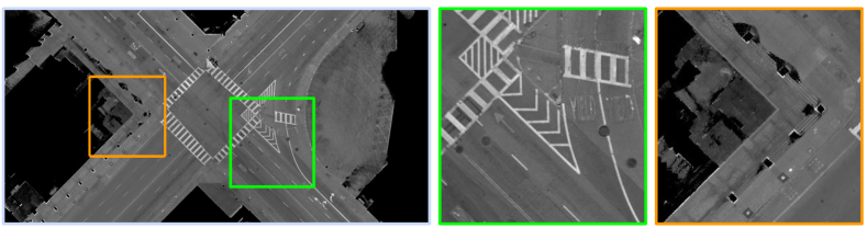
We perform high-precision localization against pre-built LiDAR intensity maps. The maps are constructed from multiple passes through the same area, which allows us to perform additional post-processing steps, such as dynamic object removal. The accumulation of multiple passes also produces maps which are much denser than individual LiDAR sweeps. The maps are encoded as orthographic bird’s eye view (BEV) images of the ground. We refer the reader to Fig. 1 for a sample fragment of the maps used by our system.
Let be the pose of the self-driving vehicle (SDV). We assume that our sensors are calibrated and neglect the effects of suspension, unbalanced tires, and vibration. This enables us to simplify the vehicle’s 6-DoF pose to only 3-DoF, namely a 2D translation and a heading angle, i.e., , where and . At each time step , our LiDAR localizer takes as input the previous pose most likely estimate and uncertainty , the vehicle dynamics , the online LiDAR image , and the pre-built LiDAR intensity map . In order to generate , we aggregate the most recent LiDAR sweeps using the IMU and wheel odometry. This produces denser online LiDAR images than just using the most recent sweep, helping localization. Since is small, drift is not an issue.
We then formulate the localization problem as deep recursive bayesian inference problem. We encode the fact that the online LiDAR sweep should be consistent with the map at the vehicle’s location, consistent with GPS readings and that the belief updates should be consistent with the motion model. Thus
| (1) |
where is a set of learnable parameters, , and are the LiDAR, GPS, and vehicle dynamics observation respectively. is the posterior distribution of the vehicle pose at time given all the sensor observations until step ; is a normalization factor. We do not need to calculate it explicitly because we discretize the belief space, so normalization is trivial.


LiDAR Matching Model:
Given a candidate pose , our LiDAR matching probability encodes the agreement between the current online LiDAR observation and the map indexed at the hypothesized pose . To compute the probability, we first project both the map and the online LiDAR intensity image into an embedding space using two deep neural networks. We then warp the online embedding according to each pose hypothesis, and compute the cross-correlation between the warped online embedding and the map embedding. Formally, this can be written as:
| (2) |
where and are the deep embedding networks of the online LiDAR image and the map, respectively, and and are the networks’ parameters. represents a 2D rigid warping function meant to transform the online LiDAR’s embedding into the map’s coordinate frame according to the given pose hypothesis . Finally, represents a cross-correlation operation.
Our embedding functions and are customized fully convolutional neural networks. The first branch takes as input the bird’s eye view (BEV) rasterized image of the most recent LiDAR sweeps (compensated by ego-motion) and produces a dense representation at the same resolution as the input. The second branch takes as input a section of the LiDAR intensity map, and produces an embedding with the same number of channels as the first one, and the spatial resolution of the map.
GPS Observation Model:
The GPS observation model encodes the likelihood of GPS observation given a location proposal. We approximate uncertainty of GPS sensory observation using a Gaussian distribution:
| (3) |
where and is the GPS observation converted from Universal Transverse Mercator (UTM) coordinate to map coordinate.
Vehicle Motion Model:
Our motion model encodes the fact that the inferred vehicle velocity should agree with the vehicle dynamics, given previous time’s belief. In particular, wheel odometry and IMU are used as input to an extended Kalman filter to generate an estimate of the velocity of the vehicle. We then define the motion model to be
| (4) |
where
| (5) |
with is a Gaussian error function. is the covariance matrix and is our three-dimensional search range centered at previous step’s . , are the 2D pose composition operator and inverse pose composition operator respectively, which, following Kümmerle et al. [35] are defined as
Network Architectures:
The and functions are computed via multi-layer fully convolutional neural networks. We experiment with a 6-layer network based on the patch matching architecture used by Luo et al. [21] and with LinkNet by Chaurasia and Culurciello [36]. We use instance normalization [37] after each convolutional layer instead of batch norm, due to its capability of reducing instance-specific mean and covariance shift. Our embedding output has the same resolution as the input image, with a (potentially) multi-dimensional embedding per pixel. The dimension is chosen based on the trade-off between performance and runtime. We refer the reader to Fig. 3 for an illustration of a single-channel embedding. All our experiments use single-channel embeddings for both online LiDAR, as well as the maps, unless otherwise stated.
3.2 Online Localization
Estimating the pose of the vehicle at each time step requires solving the maximum a posteriori problem:
| (6) |
This is a complex inference over the continuous variable , which is non-convex and requires intractable integration. These types of problems are typically solved with sampling approaches such as particle filters, which can easily fall into local minima. Moreover, most particle solvers have non-deterministic run times, which is problematic for safety-critical real-time applications like self-driving cars.
Instead, we follow the histogram filter approach to compute through a search-based method which is much more efficient, given the characteristics of the problem. To this end, we discretize the 3D search space over as a grid, and compute the term for every cell of our search space. We center the search space at the so-called dead reckoning pose , which represents the pose of the vehicle at time estimated using IMU and wheel encoders. Inference happens in the vehicle coordinate frame, with being the longitudinal offset along the car’s trajectory, , the latitudinal offset, and the heading offset. The search range is selected in order to find a compromise between the computational cost and the capability of handling large drift.
In order to do inference in real-time, we need to compute each term efficiently. The GPS term is a simple Gaussian kernel. The motion computation is quadratic w. r. t. the number of discretized states. Given the fact that it is a small neighborhood around the dead reckoning pose, the computation is very fast in practice. The most computationally demanding component of our model is the fact that we need to enumerate all possible locations in our search range to compute the LiDAR matching term . However, we observe that computing the inner product scores between two 2D deep embeddings across all translational positions in our search range is equivalent to convolving the map embedding with the online embedding as a kernel. This makes the search over and much faster to compute. As a result, the entire optimization of can be performed using convolutions, where is the number of discretization cells in the rotation () dimension.
State-of-the-art GEMM/Winograd based (spatial) GPU convolution implementations are often optimized for small convolutional kernels. Using these for the GPU-based convolutional matching implementation is still too slow for our real-time operation goal. This is due to the fact that our “convolution kernel” (i.e., the online embedding) is very large in practice (in our experiments the size of our online LiDAR embedding is , the same size as the online LiDAR image). In order to speed this up, we perform this operation in the Fourier domain, as opposed to the spatial one, according to convolution theorem: , where “” denotes an element-wise product. This reduces the theoretical complexity from to , which translates to massive improvements in terms of run time, as we will show in Section 4.
Therefore, we only need to run the embedding networks once, rotate the computed online LiDAR embedding times, and convolve each rotation with the map embedding to get the probability for all the pose hypotheses in the form of a score map . Our solution is therefore globally optimal over our discretized search space including both rotation and translation. In practice, the rotation of our online LiDAR embedding is implemented using a spatial transformer module [38], and generating all rotations takes 5ms in total (we use in all our experiments).
In order to handle robustness to observation noise and bring smooth localization results to avoid sudden jumps, we exploit a soft version of the argmax [8], which is a trade-off between center of mass and argmax:
| (7) |
where is a temperature hyper-parameter larger than 1. This gives us an estimation that takes the uncertainty of the prediction into account at time .
3.3 Learning
The localization system is end-to-end differentiable, enabling us to learn all parameters jointly using back-propagation. We find that a simple cross-entropy loss is sufficient to train the system, without requiring any additional, potentially expensive terms, such as a reconstruction loss. We define the cross-entropy loss between the ground-truth position and the inferred score map as where the labels are represented as one-hot encodings of the ground truth position, i.e., a tensor with the same shape as the score map , with a 1 at the correct pose.
 |
 |
 |
| Error vs Traveling Dist | Lateral Histogram | Longitudinal Histogram |
 |
 |
 |
| Lateral | Longitudinal | Total Translational |
4 Experimental Results
Dataset:
We collected a new dataset comprising over 4,000km of driving through a variety of urban and highway environments in multiple cities/states in North America, collected with two types of LiDAR sensors. According to the scenarios we split our dataset into Highway-LidarA and Misc-LidarB, where Highway-LidarA contains over 400 sequences for a total of over 3,000km of driving for training and validation. We select a representative and challenging subset of 282km of driving for testing, ensuring that there is no geographic overlap between the splits. All these sequences are collected by a LiDAR type A. Misc-LidarB contains 79 sequences with 200km of driving over a mix of highway and city collected by a different LiDAR type B in a different state. LiDARs A and B differ substantially in their intensity output profiles, as shown in Fig. 6.
 |
Experimental Setup:
We randomly extracted 230k training samples from the training sequences. For each training sample, we aggregate the five most recent online LiDAR sweeps to generate the BEV intensity image using vehicle dynamics, corresponding to 0.5 seconds of LiDAR scan. In such a short time drift is negligible. Our ground-truth poses are acquired through an expensive high precision offline matching procedure with up to several centimeter uncertainty. We rasterize the aggregated LiDAR points to create a LiDAR intensity image. Both the online intensity image and the intensity map are discretized at a spatial resolution of 5cm covering a region. During matching, we use the same spatial resolution, plus a rotational resolution of 0.5∘, with a total search range of ∘around the dead reckoning pose. We report the median error as well as the failure rate. The median error reflects how accurate the localization is in the majority of cases while the failure rates reflect the worst case performance In particular, we define “failure” if there is at least a frame with localization error over 1m. In addition to these per-sequence metrics, we also plot the per-frame cumulative localization error curve in Fig. 5.
| Median Error (cm) | Failure Rate (%) | |||||||
|---|---|---|---|---|---|---|---|---|
| Method | Lat | Lon | Total | m | m | End | ||
| Dynamics | Yes | No | 439.21 | 863.68 | 1216.01 | 0.46 | 98.14 | 100.00 |
| Raw LiDAR | Yes | No | 1245.13 | 590.43 | 1514.42 | 1.84 | 81.02 | 92.49 |
| ICP | Yes | No | 1.52 | 5.04 | 5.44 | 3.50 | 5.03 | 7.14 |
| Ours (LinkNet) | No | No | 3.87 | 4.99 | 7.76 | 0.35 | 0.35 | 0.72 |
| Ours (LinkNet) | Yes | No | 3.81 | 4.53 | 7.18 | 1.06 | 1.06 | 1.44 |
| Ours (LinkNet) | Yes | Yes | 3.00 | 4.33 | 6.47 | 0.00 | 0.00 | 0.00 |
| Median Error (cm) | Failure Rate (%) | |||||||
|---|---|---|---|---|---|---|---|---|
| Method | Lat | Lon | Total | m | m | End | ||
| Dynamics Only | Yes | No | 195.73 | 322.31 | 468.53 | 6.13 | 68.66 | 84.26 |
| ICP | Yes | No | 2.57 | 15.29 | 16.42 | 0.46 | 28.43 | 37.53 |
| Ours (Transfer) | Yes | No | 6.95 | 6.38 | 11.73 | 0.00 | 0.71 | 1.95 |
Implementation Details:
We manually chose the following hyper-parameters through validation, namely the motion model variance , GPS’s observation variance , temperature constant . We also conduct two ablation studies. Our first ablation verifies whether the motion prior defined in Eq. (4) is helpful. We evaluate algorithm with and without this term, denoted as in Table 1. Our second ablation evaluates whether a probabilistic MLE proposed in Eq. (7) helps improve performance, denoted as . The none-probabilistic is achieved through changing the soft-argmax in Eq. (7) to a hard argmax. We implement our full inference algorithm in PyTorch 0.4. The networks are trained using Adam over four NVIDIA 1080Ti GPUs with initial learning rate at 0.001.
Comparison to Other Methods:
We compare our algorithm against several baselines. The raw matching consists of performing the matching-based localization in a similar manner to our method but only use the raw intensity BEV online and map images, instead of the learned embeddings. The ICP baseline conducts point-to-plane ICP between the raw 3D LiDAR points against the 3D pre-scanned localization prior at 10Hz, initialized in a similar manner as us using the previous estimated location plus the vehicle dynamics. This ensures good quality of initialization, as required by algorithms from ICP family.
Localization Performance:
As shown in Table 1, our approach achieves the best performance among all the competing algorithms in terms of failure rate. Both probabilistic inference and motion prior further improves the robustness of our method. Our ICP baseline is competitive in terms of median error, especially along lateral direction, but the failure rate is significantly higher. It is also more computationally demanding and requires 3D maps. Both dynamics-only and raw intensity matching result in large drift. Moreover, we have observed that deeper architectures and the probabilistic inference are generally helpful. Fig. 4 shows the localization error as a function of the travel distance aggregated across all sequences from the Highway-LidarA test set. The solid line denotes the median and the shaded region denotes the area, together with the distribution of lateral and longitudinal errors per frame. Fig. 5 compares our approach to ICP in terms of cumulative errors with -percentile error reported. From this we can see our method significantly outperforms ICP in terms of the worst-case behavior.
Domain Shift:
In order to show that our approach generalize well across LiDAR sensors, we conduct a second experiment, where we train our network on Highway-LidarA, which is purely highway, collected using LiDAR A, and test on the test set of Misc-LidarB which is highway + city, collected by a different LiDAR (type B) in a different state. In order to better highlight the difference, in Fig. 6 we show two LiDARs intensity value distributions and their raw intensity images, collected at the same location. Table 2 showcases the results of this experiment. From the table we can see our neural network is able to generalize both across LiDAR models and across environment types.
Runtime Analysis:
We conduct a runtime analysis over both embedding networks and matching. Our LinkNet based embedding networks take less than 10ms each for a forward pass over both online and map images. We also compare the cuDNN implementation of FFT-conv and standard spatial convolution. FFT reduces the run time of the matching by an order of magnitude bringing it down from to for a single-channel embedding. This enables us to run the localization algorithm at 15 Hz, thereby achieving our real-time operation goal.
5 Conclusion
We proposed a real-time, calibration-agnostic, effective localization method for self-driving cars. Our method projects the online LiDAR sweeps and intensity map into a joint embedding space. Localization is conducted through efficient convolutional matching between the embeddings. This approaches allows our full system to operate in real-time at 15Hz while achieving centimeter-level accuracy without intensity calibration. The method also generalizes well to different LiDAR types without the need to re-train. The experiments illustrate the performance of the proposed approach over two comprehensive test sets covering over 500km of driving in diverse conditions.
Acknowledgments
We would like to thank Min Bai, Julieta Martinez, Joyce Yang, and Shrinidhi Kowshika Lakshmikanth for their help with proofreading, experiments, and dataset generation. We would also like to thank our anonymous reviewers for the detailed feedback they provided on our work, which helped us improve our system and paper in multiple ways.
References
- Besl and McKay [1992] P. J. Besl and N. D. McKay. Method for registration of 3-d shapes. In Sensor Fusion IV: Control Paradigms and Data Structures, 1992.
- Rusinkiewicz and Levoy [2001] S. Rusinkiewicz and M. Levoy. Efficient variants of the icp algorithm. In 3DIM, 2001.
- Cummins and Newman [2008] M. Cummins and P. Newman. Fab-map: Probabilistic localization and mapping in the space of appearance. IJRR, 2008.
- Ziegler et al. [2014] J. Ziegler, H. Lategahn, M. Schreiber, C. G. Keller, C. Knoppel, J. Hipp, M. Haueis, and C. Stiller. Video based localization for bertha. In IV, 2014.
- Arandjelovic et al. [2016] R. Arandjelovic, P. Gronat, A. Torii, T. Pajdla, and J. Sivic. Netvlad: Cnn architecture for weakly supervised place recognition. In CVPR, 2016.
- Sattler et al. [2017] T. Sattler, A. Torii, J. Sivic, M. Pollefeys, H. Taira, M. Okutomi, T. Pajdla, T. Sattler, A. Torii, J. Sivic, M. Pollefeys, H. Taira, and A. Large-scale. Are Large-Scale 3D Models Really Necessary for Accurate Visual Localization? pages 1637–1646, 2017. doi:10.1109/CVPR.2017.654.
- Levinson et al. [2007] J. Levinson, M. Montemerlo, and S. Thrun. Map-based precision vehicle localization in urban environments. In RSS, 2007.
- Levinson and Thrun [2010] J. Levinson and S. Thrun. Robust vehicle localization in urban environments using probabilistic maps. In ICRA, 2010.
- Engel et al. [2014] J. Engel, T. Schöps, and D. Cremers. Lsd-slam: Large-scale direct monocular slam. In ECCV, 2014.
- Mur-Artal et al. [2015] R. Mur-Artal, J. M. M. Montiel, and J. D. Tardos. Orb-slam: a versatile and accurate monocular slam system. IEEE Transactions on Robotics, 2015.
- Zhang and Singh [2014] J. Zhang and S. Singh. Loam: Lidar odometry and mapping in real-time. In RSS, 2014.
- Brubaker et al. [2013] M. Brubaker, A. Geiger, and R. Urtasun. Lost! leveraging the crowd for probabilistic visual self-localization. In CVPR, 2013.
- Ma et al. [2017] W.-C. Ma, S. Wang, M. A. Brubaker, S. Fidler, and R. Urtasun. Find your way by observing the sun and other semantic cues. In ICRA, 2017.
- Wolcott and Eustice [2015] R. W. Wolcott and R. M. Eustice. Fast LIDAR localization using multiresolution Gaussian mixture maps. In ICRA, 2015.
- Wolcott and Eustice [2014] R. W. Wolcott and R. M. Eustice. Visual localization within lidar maps for automated urban driving. In IROS, 2014.
- Schreiber et al. [2013] M. Schreiber, C. Knöppel, and U. Franke. Laneloc: Lane marking based localization using highly accurate maps. In IV, 2013.
- Yoneda et al. [2014] K. Yoneda, H. Tehrani, T. Ogawa, N. Hukuyama, and S. Mita. Lidar scan feature for localization with highly precise 3-d map. In IV, 2014.
- Wan et al. [2017] G. Wan, X. Yang, R. Cai, H. Li, H. Wang, and S. Song. Robust and Precise Vehicle Localization based on Multi-sensor Fusion in Diverse City Scenes. arXiv, 2017.
- Thrun and Montemerlo [2006] S. Thrun and M. Montemerlo. The graph slam algorithm with applications to large-scale mapping of urban structures. IJRR, 2006.
- Zbontar and LeCun [2015] J. Zbontar and Y. LeCun. Computing the stereo matching cost with a convolutional neural network. In CVPR, 2015.
- Luo et al. [2016] W. Luo, A. G. Schwing, and R. Urtasun. Efficient deep learning for stereo matching. In CVPR, 2016.
- Han et al. [2015] X. Han, T. Leung, Y. Jia, R. Sukthankar, and A. C. Berg. Matchnet: Unifying feature and metric learning for patch-based matching. In CVPR, 2015.
- Xu et al. [2017] J. Xu, R. Ranftl, and V. Koltun. Accurate optical flow via direct cost volume processing. CVPR, 2017.
- Bai et al. [2016] M. Bai, W. Luo, K. Kundu, and R. Urtasun. Exploiting semantic information and deep matching for optical flow. In ECCV, 2016.
- Zagoruyko and Komodakis [2015] S. Zagoruyko and N. Komodakis. Learning to compare image patches via convolutional neural networks. In CVPR, 2015.
- Zeng et al. [2017] A. Zeng, S. Song, M. Nießner, M. Fisher, J. Xiao, and T. Funkhouser. 3dmatch: Learning local geometric descriptors from rgb-d reconstructions. In CVPR, 2017.
- Shotton et al. [2013] J. Shotton, B. Glocker, C. Zach, S. Izadi, A. Criminisi, and A. Fitzgibbon. Scene coordinate regression forests for camera relocalization in rgb-d images. In CVPR, 2013.
- Wang et al. [2015] S. Wang, S. Fidler, and R. Urtasun. Lost shopping! monocular localization in large indoor spaces. In ICCV, 2015.
- Kendall et al. [2015] A. Kendall, M. Grimes, and R. Cipolla. Posenet: A convolutional network for real-time 6-dof camera relocalization. In ICCV, 2015.
- Zhou et al. [2017] T. Zhou, M. Brown, N. Snavely, and D. G. Lowe. Unsupervised learning of depth and ego-motion from video. arXiv, 2017.
- Wang et al. [2017] S. Wang, R. Clark, H. Wen, and N. Trigoni. Deepvo: Towards end-to-end visual odometry with deep recurrent convolutional neural networks. In ICRA, 2017.
- Bloesch et al. [2018] M. Bloesch, J. Czarnowski, R. Clark, S. Leutenegger, and A. J. Davison. Codeslam-learning a compact, optimisable representation for dense visual slam. CVPR, 2018.
- Brachmann and Rother [2017] E. Brachmann and C. Rother. Learning Less is More - 6D Camera Localization via 3D Surface Regression. arXiv, 2017.
- Radwan et al. [2018] N. Radwan, A. Valada, and W. Burgard. VLocNet++: Deep Multitask Learning for Semantic Visual Localization and Odometry. arXiv, 2018.
- Kümmerle et al. [2009] R. Kümmerle, B. Steder, C. Dornhege, M. Ruhnke, G. Grisetti, C. Stachniss, and A. Kleiner. On measuring the accuracy of slam algorithms. Autonomous Robots, 27(4):387, 2009.
- Chaurasia and Culurciello [2017] A. Chaurasia and E. Culurciello. Linknet: Exploiting encoder representations for efficient semantic segmentation. arXiv, 2017.
- Ulyanov et al. [2016] D. Ulyanov, A. Vedaldi, and V. S. Lempitsky. Instance normalization: The missing ingredient for fast stylization. arXiv, 2016.
- Jaderberg et al. [2015] M. Jaderberg, K. Simonyan, A. Zisserman, et al. Spatial transformer networks. In NIPS, 2015.
Appendix A Supplementary Material
A.1 Additional Ablation Study Results
Embedding Dimensions:
We also investigate the impact that the number of embedding channels has on matching performance and the runtime of the system. Table 3 shows the performance. As shown in this table, increasing the number of channels in the embeddings does not improve performance by a significant amount, whereas reducing the number of channels could reduce the runtime of matching by a large margin, which favors relative low-dimensionality in practice. Therefore, using single-channel embeddings (just like the input intensity images) is adequate.
Network Architectures
We experiment with two configurations of embedding networks. The first one, denoted as FCN, uses the shallow network described in Section 3 for both online and map branches. The second architecture uses a LinkNet [36] architecture for both the online and the map branches. The results are reported in Table 4. From the table, we can see LinkNet achieves better performance than FCN and the motion model consistently helps when using either architecture.
Reduced Training Dataset Size:
Given that the matching task is conceptually straightforward, requiring far less high-level reasoning capabilities compared to problems such as semantic segmentation, we perform a series of experiments where we train our matching network using smaller samples of our training dataset, and investigate the localization performance of our system in these cases. These results are presented in Table 5.
| Method | Matching Accuracy | Inference Time (ms) | |||
|---|---|---|---|---|---|
| Backbones | Matching (Slow) | Matching (FFT) | |||
| Raw matching | 13.95% | n/A | 26.66ms | 1.43ms | |
| 1 channel | 71.97% | 19.34ms | 26.66ms | 1.43ms | |
| 2 channels | 72.08% | 17.16ms | 55.03ms | 6.60ms | |
| 4 channels | 71.67% | 16.70ms | 110.46ms | 11.18ms | |
| 8 channels | 71.63% | 18.08ms | 168.96ms | 21.64ms | |
| 12 channels | 72.50% | 18.73ms | 330.75ms | 32.93ms | |
| Median Error (cm) | Failure Rate (%) | |||||||
|---|---|---|---|---|---|---|---|---|
| Method | Lat | Lon | Total | m | m | End | ||
| Ours (FCN) | No | No | 4.41 | 4.86 | 8.01 | 0.35 | 0.35 | 0.71 |
| Ours (FCN) | Yes | Yes | 5.50 | 6.00 | 9.52 | 1.06 | 1.42 | 2.52 |
| Ours (LinkNet) | No | No | 3.87 | 4.99 | 7.76 | 0.35 | 0.35 | 0.72 |
| Ours (LinkNet) | Yes | Yes | 3.19 | 4.86 | 7.09 | 0.00 | 0.00 | 0.35 |
| Median Error (cm) | Failure Rate (%) | |||||||
|---|---|---|---|---|---|---|---|---|
| Method | Lat | Lon | Total | m | m | End | ||
| LinkNet, 100% of data | Yes | Yes | 3.19 | 4.86 | 7.09 | 0.00 | 0.00 | 0.35 |
| LinkNet, 25% of data | Yes | Yes | 2.92 | 5.33 | 7.24 | 0.00 | 0.00 | 1.08 |
| LinkNet, 5% of data | Yes | Yes | 3.95 | 6.76 | 9.25 | 1.06 | 1.06 | 2.52 |
| LinkNet, 1% of data | Yes | Yes | 4.66 | 8.70 | 11.40 | 0.71 | 2.14 | 3.60 |
A.2 Additional Qualitative Results
A.3 Qualitative Results
Fig. 7 qualitatively compares the localization accuracy of our method with those discussed in the previous section. For further qualitative results, please refer to the video associated with this paper.


