Learning to Affiliate: Mutual Centralized Learning for Few-shot Classification

In a $N$-way $K$-shot episode, the goal is to predict a class label for a single query image given $N$ support classes, each of which contains $K$ support images for reference.

We first encode each input image into $r$ number of $d$-dimensional dense features $f_{\theta}(\cdot)\in\mathbb{R}^{d\times r}$. We use $\mathbf{q}=\{q_{1},...,q_{r}\}$ to denote dense features from a query image. Inspired by prototype learning [26], we average feature vectors from the same spatial locations of $K$ different images into support dense features for each $\mathbf{s}^{c}=\{s_{1}^{c},...,s_{r}^{c}\}$ category.

We use the bold font (e.g., $\mathbf{q}$ and $\mathbf{s}$) to denote a set of feature vectors and use the normal font (e.g., $q$ and $s$) to denote a single feature vector. We use $\mathbf{S}=\bigcup_{c\in C}\mathbf{s}^{c}$ to represent the union set of dense features from all supporting classes. The cardinalities for the sets $\mathbf{q}$, $\mathbf{s}^{c}$ and $\mathbf{S}$ are $r$, $r$ and $Nr$ respectively.

The target of dense features based FSL is to find the label of a query image, given its dense query features $\mathbf{q}$ and the union set of dense support features $\mathbf{S}$ from all categories.

We start by using the cosine similarity $\phi(v_{1},v_{2})=\langle\frac{v_{1}}{\|v_{1}\|},\frac{v_{2}}{\|v_{2}\|}\rangle$ to measure the closeness between the two feature vectors where $\langle\cdot,\cdot\rangle$ is the Frobenius inner product.

Given two dense features sets $\mathbf{q}$ and $\mathbf{S}$, we learn inter similarity matrix $\mathbf{\Phi}\in\mathbb{R}^{r\times Nr}$ between those two disjoint sets where the entry of $\left[\mathbf{\Phi}\right]_{qs}=\phi(q,s)$ indicates the similarity between vectors $q\in\mathbf{q}$ and $s\in\mathbf{S}$.

We build query-to-support affiliations from every query feature $q$ to all support features $s\in\mathbf{S}$ by a random walk probability $p_{sq}=\frac{e^{\gamma\phi(s,q)}}{\sum_{s^{\prime}\in\mathbf{S}}e^{\gamma\phi(s^{\prime},q)}}$. The probability matrix from all query to support features can be written by

where $\mathrm{exp}(\cdot)$ is the element-wise exponential function, $\gamma$ is a scaling temperature for a softmax like probability and $\mathbf{D}$ is a diagonal normalization matrix with its $(j,j)$-value to be the sum of the $j$-th column of $\mathrm{exp}(\gamma\mathbf{\Phi}^{\mathrm{T}})$. The subscript serves both as the matrix size and as an indication for the feature vector with which it is associated. For example, $\mathbf{P}_{\mathbf{Sq}}$ is of size $|\mathbf{S}|\times|\mathbf{q}|$ and it includes random walk probabilities from query features $\mathbf{q}$ to support features $\mathbf{S}$.

Likewise, we connect every support feature $s$ to all $q\in\mathbf{q}$ by a similar probability matrix:

where $\mathbf{W}$ is the analogous diagonal matrix with its $(j,j)$-value to be the sum of the $j$-th column of $\mathrm{exp}(\beta\mathbf{\Phi})$.

It should be noted that we use two different scaling parameters since $\mathbf{\Phi}$ is a non-square matrix due to the different cardinalities of dense feature sets $\mathbf{q}$ and $\mathbf{S}$. Although the matrices $\mathrm{exp}(\gamma\mathbf{\Phi}^{\mathrm{T}})$ and $\mathrm{exp}(\beta\mathbf{\Phi})$ would be symmetric if we ignore their different scaling parameters, the probability matrices $\mathbf{P}_{\mathbf{qS}}$, $\mathbf{P}_{\mathbf{Sq}}$ are both column-normalized by different $\mathbf{D}$, $\mathbf{W}$ respectively and are thus directional.

To learn the mutual affiliations between the two dense feature sets, we first associate each feature vector with a particle $z$ that forms a discrete feature space $\mathbf{z}=\mathbf{q}\cup\mathbf{S}$. Next, we let particles bidirectionally random walk between particles in that space according to $\mathbf{P}_{\mathbf{Sq}}$ and $\mathbf{P}_{\mathbf{qS}}$ (i.e., particles at query features set are only allowed to move to the support features set, and vice versa). We assume it time-homogeneous in a Markov process $\{X_{t}\}$ and the random walk probability from $z_{j}$ to $z_{i}$ for all $z_{i}$, $z_{j}$ in $\mathbf{z}$ can be formulated by:

To write it in matrix, we can obtain the Markov transition matrix $\mathbf{P}$:

that consists of the column-normalized $\mathbf{P}_{\mathbf{Sq}}$ and $\mathbf{P}_{\mathbf{qS}}$.

It can be proved (in supplementary) that, after infinity times of bidirectional random walks, the Markov chain with anti-diagonal $\mathbf{P}$ reaches the periodic stationary distribution:

where $\bm{\pi}(\mathbf{S})\in\mathbb{R}^{Nr}$, $\bm{\pi}(\mathbf{q})\in\mathbb{R}^{r}$ are the stationary distributions with equations $\bm{\pi}(\mathbf{S})=\mathbf{P_{Sq}}\mathbf{P_{qS}}\bm{\pi}(\mathbf{S})$ and $\bm{\pi}(\mathbf{q})=\mathbf{P_{qS}P_{Sq}}\bm{\pi}(\mathbf{q})$ respectively. $\bm{e}_{|\cdot|}$ is a vector of ones with different length indicated by its subscript.

The motivation of using these stationary distributions to encode mutual affiliations is straightforward: support features would be frequently visited in the long times of bidirectional random walk if they shared the same local characteristics with the query ones. In other words, the support class that owns the most mutual affiliations with querying image would be predicted due to their mutual closeness.

To formulate it in FSL, we first assume particles are uniformly distributed in the discrete finite space $\mathbf{z}$. Then, we use the expected number of visits from all particles $z\in\mathbf{z}$ to support features $\mathbf{s}^{c}\subset\mathbf{S}$ of class $c$ in the long times of bidirectional random walks $\{X_{t}\}$ to measure the amount of local characteristics that class $c$ owns for the query image:

where $\mathds{1}[\cdot]$ is an indicator function that equals 1 if its argument is true and zero otherwise. $[\cdot]_{ij}$ indicates the entry of the matrix from particle $j$ to particle $i$ and $[\cdot]_{i}$ indicates the entry of the vector that associated to feature $i$.

We give the derivation when the Markov chain length $t$ is even in the first equality of Eqn.(LABEL:eq:MEL) and prove that the odd $t$ reaches the same result in the supplementary material. The second equality is from the absorbing property of the periodic Markov chain where the power of matrix gets saturated to Eqn.(5) for the increasing $t$. Since $\bm{\pi}(\mathbf{S})$ is the stationary distribution of column-stochastic $\mathbf{P_{Sq}P_{qS}}$ under the probability constraint $\bm{e}^{\mathrm{T}}_{Nr}\bm{\pi}(\mathbf{S})=1$, $\mathbf{Pr}(\tilde{y})$ is a valid distribution for classifications.

If we interpret the random walk probability matrix $\mathbf{P}$ as an adjacency matrix $\{a_{v_{1},v_{2}}\}$ of a directed bipartite graph $G:=(V=\{\mathbf{q},\mathbf{S}\},E)$, we find that the dense features’ accessibility in the time-homogeneous bidirectional random walk would be equivalent to learning a single-mode eigenvector centrality on the graph $G$. The bipartite graph is also called the affiliation network in social network analysis [3, 4, 5] that models two types of entities "actors" and "society" related by affiliation of the former in the latter. The concept of centrality in social network analysis is generally used to investigate the acquaintanceships among people that often stem from one or more shared affiliations.

To see this in graph theory, we start with a brief overview of the eigenvector centrality that reflects score $x$ of vertex $v$ for both $q\in\mathbf{q}$ and $s\in\mathbf{S}$ in the affiliation network with adjacency $\{a_{v_{1},v_{2}}\}$:

where $\mathbb{V}(\cdot)$ is a set of neighbors for the given vertex and $\lambda$ is a constant.

With a small rearrangement, Eqn.(7) can be rewritten in vector notation with an eigenvector equation $\mathbf{Px}=\lambda\mathbf{x}$. The additional requirement that all the entries of the eigenvector be non-negative implies (by the Perron–Frobenius theorem [21]) that only the greatest eigenvalue results in the desired centrality measure. For the column-stochastic adjacency matrix $\mathbf{P}$ in our method, the largest eigenvalue $\lambda$ is 1.

Single-mode centrality [5] is a special form of graph centrality that measures the extent to which nodes in one vertex set are relatively central only to other nodes in the same vertex set on bipartite graph. For example, the single-mode centrality for different $s$ in $\mathbf{S}$ is defined by $\hat{\mathbf{x}}_{\mathbf{S}}=\mathbf{x}_{\mathbf{S}}/\sum_{s\in\mathbf{S}}x_{s}$. Lemma 1 (proved in supplementary material) shows that dense features’ accessibility $\bm{\pi}(\mathbf{S})$ of bidirectional random walks in Eqn.(LABEL:eq:MEL) is equivalent to the single-mode eigenvector centrality of support set $\mathbf{S}$ on bipartite data.

Based on this reinterpretation, it is straightforward to introduce the attenuation (damping) factor $\alpha$ in Markov bidirectional random walks motivated by the Katz centrality [13], where connections made with distant neighbors are penalized by $\alpha$. The dense features’ accessibility with attenuation factor $\alpha$ for few-shot classifications is defined by

where $\epsilon=(Nr+r)\sum_{t=1}^{\infty}\alpha^{t}=(Nr+r)\alpha/(1-\alpha)$ is a constant for a valid distribution.

Although we simply consider the single-mode centrality on $\mathbf{S}$ for an end-to-end classification purpose, it is also beneficial to learn its conjugate centrality $\bm{\pi}(\mathbf{q})$ on $\mathbf{q}$ in the affiliation network (by the analogous $\bm{\pi}(\mathbf{q})=\mathbf{x}_{\mathbf{q}}/\sum_{q\in\mathbf{q}}x_{q}$ in Lemma 1). We will show that both single-mode centralities on two dense features sets could serve as plug-and-play for finding centralized local characteristics in existing methods (hence the term Mutual Centralized Learning, MCL).

The algorithm of Mutual Centralized Learning (MCL) in Eqn.(LABEL:eq:MEL) involves the computation of Markov stationary distribution $\bm{\pi}(\mathbf{S})$ with equation $\bm{\pi}(\mathbf{S})=\mathbf{P_{Sq}P_{qS}}\bm{\pi}(\mathbf{S})$. Theoretically, the $\bm{\pi}(\mathbf{S})$ is the eigenvector of $\mathbf{P_{Sq}P_{qS}}$ with the eigenvalue 1 under a probability constraint $\bm{e}_{Nr}^{\mathrm{T}}\bm{\pi}(\mathbf{S})=1$.

The above constraints could lead to a solution of $\bm{\pi}(\mathbf{S})$ by solving the overdetermined linear system

where $\bm{I}$ is an identity matrix and $\mathbf{0}$ is a vector of zeros. Although we can solve it by various methods like pseudo-inverse or QR decomposition and back substitution, it is empirically found time-consuming as these operators are either numerically unstable or not paralleled well in modern deep-learning packages.

To handle it, we present an alternative solution based on Lemma 1 as follows: We first calculate the Katz centrality by its closed-form solution [13]:

and then solve single-mode Katz centrality in Eqn.(8) by the definition of the single-mode centrality:

Since Katz centrality degrades to the eigenvector centrality when $\alpha$ approaches 1 [13] (indicates no attenuation), we can obtain the approximation of eigenvector centrality by a large $\alpha=0.999$:

and the analogous single-mode eigenvector centrality in Eqn.(LABEL:eq:MEL) can then be approximated by:

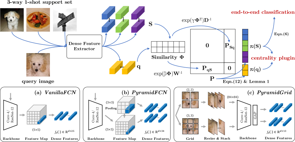
We use the negative log-likelihood loss to update parameters in different feature extractors and the whole picture of MCL for few-shot classifications is shown in Figure 2. We provide the detailed algorithm/pseudo-codes in the supplementary material for reference.

Since the underlying centrality learned by MCL reveals the different importance of local features on an affiliation network, it is thus plausible to plug it into global feature based methods by replacing their native global average pooling (GAP) with the centrality weighted pooling as follows:

a. Extract dense features for each input image.

b. Compute the eigenvector centrality $\mathbf{x}^{\mathrm{Eigen}}$ by Eqn.(12).

c. Compute $\bm{\pi}(\mathbf{S})$ and $\bm{\pi}(\mathbf{q})$ according to definition of the single-mode centrality in Lemma 1.

d. Use $\bm{\pi}(\mathbf{q})$ as weights on query dense features and weighted accumulate them to a single feature vector.

e. Use the class-wise normalized centrality from $\bm{\pi}(\mathbf{S})$ to accumulate dense features for each supporting class.

Once we get the centrality weighted features for the query image and support classes, it is straightforward to perform traditional global feature based methods like before.

Table 1 details the comparisons of MCL with global feature based methods [25, 14, 34, 7, 19] as well as dense feature based methods [16, 35, 33] on mini-/tieredImageNet.

Besides these methods, we also exploit label propagation [36] in dense feature based inductive FSL like in [17] to demonstrate that traditional transductive methods could be easily adapted to inductive settings if we treat dense feature vectors as a set of unlabeled data. As shown, our MCL is highly competitive with recent state-of-the-art results. In particular, our MCL-Katz achieves 67.51% (1-shot) and 83.99% (5-shot) on miniImageNet with the simplest VanillaFCN.

Comparisons with dense feature based methods. The last three panes of Table 1 illustrate that proposed bidirectional MCL outperforms query-to-support DN4’s nearest neighboring, DeepEMD’s optimal matching and FRN’s latent feature reconstructions in various tasks. Although the optimal matching flow is unidirectional in DeepEMD, they adopt a cross-reference attention that encodes the bidirectional relevance to a certain extent. If we treat dense features as nodes in the graph and use their similarities as edges, a major difference is that they treat nodes equally to derive different weights on edges while we use the fixed edges to derive the centrality of nodes directly for classifications.

Comparisons with global feature based methods. The centrality investigated in this work is also capable to be plugged into global feature based methods as local features are not equally important before global average pooling. As shown in the first pane of Table 1, our proposed centrality weighted pooling could provide at most 3.4% and 4.5% performance gains for ProtoNet and RelationNet respectively. We show in Table 4 that the improvements are also consistent if we solely apply it on the query and support dense features.

We follow the same setting (shown in supplementary) as in FRN [33] to train all the models from scratch on those fine-grained datasets. We re-implement DN4 [16], DeepEMD [35] to thoroughly compare with dense features based methods. Apart from the basic comparisons (both backbones on CUB and Conv-4 backbone on meta-iNat/tiered-meta-iNat) in [33], we conduct extra ResNet-12 experiments for all the comparing methods on meta-iNat and tiered-meta-iNat in our unified framework for a thorough comparison.

Results in Table 2 demonstrate that both our end-to-end MCL (VanillaFCN) and the centrality plugin are broadly effective in various fine-grained few-shot classification tasks.

Different choices of $\gamma$,$\beta$. Since $\mathbf{\Phi}$ is non-square due to the different cardinalities of set $\mathbf{S}$ and $\mathbf{q}$, we use two different scaling parameters in Eqn.(1) and Eqn.(2). By the column-wise normalization, $\gamma$ and $\beta$ can be interpreted as the reciprocal of temperatures in softmax random walk probability. Large $\gamma$, $\beta$ will have a hard random walk probability that leads to a concentrated centrality in the affiliation network. However, extremely large $\gamma$, $\beta$ (e.g., one-hot probability when they approaching infinity) would inevitably bias the episodic training due to the potential gradient explosion.

Since the cardinality of set $\mathbf{S}$ is larger than that of $\mathbf{q}$, we empirically use a larger $\gamma$ than $\beta$ as we need a harder probability in random walks from query to the large set of support features. In the experiments, we carefully select $\gamma$ and $\beta$ (generally $\gamma$=$20$ and $\beta$=$10$ for 1-shot models and $\gamma$=$40$ and $\beta$=$20$ for 5-shot models) from several combinations of parameters by their validation performance.

Influence of Katz attenuation factor $\alpha$. When $\alpha$ is small, the contribution given by paths longer than one rapidly declines, and the centrality will be determined by short paths (mostly in-degrees). When $\alpha$ is large, long paths are devalued smoothly, and the centrality would be more influenced by endogenous topology. When $\alpha$ approaching 0, the classification will be only determined by the unidirectional query-to-support random walk where the contributions from paths longer than one just vanished. We show comparisons in Table 3 to demonstrate that performances are improved by introducing mutual affiliations in a bidirectional manner.

In the experiments, we simply use $\alpha=0.5$ for MCL-Katz methods, and the performances could be further improved by selecting different $\alpha$ as shown in supplementary.

Intuitively, bidirectional methods would be slower than unidirectional ones since their back-and-forth computations. However, our MCL would definitely reach to the periodic equilibrium state as shown in Eqn.(5). Thus, we could directly solve it by the Katz approximation.

At first glance, the most expensive step in Eqn.(10) is inverting $\bm{I}-\alpha\mathbf{P}$ that costs $O(N^{3}r^{3})$ where $N$ is the number of supporting classes and $r$ is the number of dense features for each image input. Fortunately, $\bm{I}-\alpha\mathbf{P}$ is a very special matrix that equals a diagonal matrix minus an anti-diagonal matrix. In this case, we can reformulate it by block-wise matrix inversion:

where $\mathbf{\Delta}$ is defined by $\bm{I}-\alpha^{2}\mathbf{P_{Sq}}\mathbf{P_{qS}}$. The most expensive step then becomes a inversion of $\mathbf{\Delta}\in\mathbb{R}^{r\times r}$ and the time complexity is reduced to $O(r^{3})$.

As shown in Table 6, we compare the inference speed between MCL and other unidirectional dense feature based methods with different image resolutions on 5-way 1-shot FSL tasks with ResNet-12. Each class contains 15 query images in an episode. It can be observed that our bidirectional MCL did not introduce many computational overheads compared to unidirectional methods, and Katz approximation does accelerate computing the stationary distribution.

To better understand our centrality based methods, we visualize the Grad-CAM [24] of the last convolutional layer in ResNet-12 for both plugin and end-to-end methods. We show in Table 5(a) that our MCL helps ProtoNet concentrate on the most relevant regions of interest. Table 5(b) demonstrates that the most centralized support features in MCL are not only from the ground truth but also mutually affiliated with task-relevant objects in the query images. We consider it qualitatively validates our underlying idea that support features would be frequently visited in the long times of bidirectional random walks if they shared the same local characteristics with the query image.

References

- [1] Arman Afrasiyabi, Jean-François Lalonde, and Christian Gagn’e. Associative alignment for few-shot image classification. In European Conference on Computer Vision, pages 18–35. Springer, 2020.
- [2] Luca Bertinetto, Joao F Henriques, Philip Torr, and Andrea Vedaldi. Meta-learning with differentiable closed-form solvers. In International Conference on Learning Representations, 2018.
- [3] Phillip Bonacich. Factoring and weighting approaches to status scores and clique identification. Journal of mathematical sociology, 2(1):113–120, 1972.
- [4] Phillip Bonacich. Simultaneous group and individual centralities. Social networks, 13(2):155–168, 1991.
- [5] Stephen P Borgatti and Martin G Everett. Network analysis of 2-mode data. Social networks, 19(3):243–269, 1997.
- [6] Wei-Yu Chen, Yen-Cheng Liu, Zsolt Kira, Yu-Chiang Frank Wang, and Jia-Bin Huang. A closer look at few-shot classification. In International Conference on Learning Representations, 2019.
- [7] Yinbo Chen, Xiaolong Wang, Zhuang Liu, Huijuan Xu, and Trevor Darrell. A new meta-baseline for few-shot learning. arXiv preprint arXiv:2003.04390, 2020.
- [8] Guneet Singh Dhillon, Pratik Chaudhari, Avinash Ravichandran, and Stefano Soatto. A baseline for few-shot image classification. In International Conference on Learning Representations, 2019.
- [9] Kaize Ding, Jianling Wang, Jundong Li, Kai Shu, Chenghao Liu, and Huan Liu. Graph prototypical networks for few-shot learning on attributed networks. In Proceedings of the 29th ACM International Conference on Information & Knowledge Management, pages 295–304, 2020.
- [10] Carl Doersch, Ankush Gupta, and Andrew Zisserman. Crosstransformers: spatially-aware few-shot transfer. arXiv preprint arXiv:2007.11498, 2020.
- [11] Victor Garcia and Joan Bruna. Few-shot learning with graph neural networks. arXiv preprint arXiv:1711.04043, 2017.
- [12] Fusheng Hao, Fengxiang He, Jun Cheng, Lei Wang, Jianzhong Cao, and Dacheng Tao. Collect and select: Semantic alignment metric learning for few-shot learning. In Proceedings of the IEEE/CVF International Conference on Computer Vision, pages 8460–8469, 2019.
- [13] Leo Katz. A new status index derived from sociometric analysis. Psychometrika, 18(1):39–43, 1953.
- [14] Kwonjoon Lee, Subhransu Maji, Avinash Ravichandran, and Stefano Soatto. Meta-learning with differentiable convex optimization. In Proceedings of the IEEE/CVF Conference on Computer Vision and Pattern Recognition, pages 10657–10665, 2019.
- [15] Wenbin Li, Lei Wang, Jing Huo, Yinghuan Shi, Yang Gao, and Jiebo Luo. Asymmetric distribution measure for few-shot learning. In Proceedings of the Twenty-Ninth International Conference on International Joint Conferences on Artificial Intelligence, pages 2957–2963, 2021.
- [16] Wenbin Li, Lei Wang, Jinglin Xu, Jing Huo, Yang Gao, and Jiebo Luo. Revisiting local descriptor based image-to-class measure for few-shot learning. In Proceedings of the IEEE/CVF Conference on Computer Vision and Pattern Recognition, pages 7260–7268, 2019.
- [17] Yann Lifchitz, Yannis Avrithis, and Sylvaine Picard. Local propagation for few-shot learning. In 2020 25th International Conference on Pattern Recognition (ICPR), pages 10457–10464. IEEE, 2021.
- [18] Yann Lifchitz, Yannis Avrithis, Sylvaine Picard, and Andrei Bursuc. Dense classification and implanting for few-shot learning. In Proceedings of the IEEE/CVF Conference on Computer Vision and Pattern Recognition, pages 9258–9267, 2019.
- [19] Bin Liu, Yue Cao, Yutong Lin, Qi Li, Zheng Zhang, Mingsheng Long, and Han Hu. Negative margin matters: Understanding margin in few-shot classification. In European Conference on Computer Vision, pages 438–455. Springer, 2020.
- [20] Yanbin Liu, Juho Lee, Minseop Park, Saehoon Kim, Eunho Yang, Sung Ju Hwang, and Yi Yang. Learning to propagate labels: Transductive propagation network for few-shot learning. In International Conference on Learning Representations, 2019.
- [21] Oskar Perron. Zur theorie der matrices. Mathematische Annalen, 64(2):248–263, 1907.
- [22] Mengye Ren, Eleni Triantafillou, Sachin Ravi, Jake Snell, Kevin Swersky, Joshua B Tenenbaum, Hugo Larochelle, and Richard S Zemel. Meta-learning for semi-supervised few-shot classification. In International Conference on Learning Representations, 2018.
- [23] Ravi Sachin and Larochell Hugo. Optimization as a model for few-shot learning. ICLR, 2017.
- [24] Ramprasaath R Selvaraju, Michael Cogswell, Abhishek Das, Ramakrishna Vedantam, Devi Parikh, and Dhruv Batra. Grad-cam: Visual explanations from deep networks via gradient-based localization. In Proceedings of the IEEE international conference on computer vision, pages 618–626, 2017.
- [25] Christian Simon, Piotr Koniusz, Richard Nock, and Mehrtash Harandi. Adaptive subspaces for few-shot learning. In CVPR, pages 4136–4145, 2020.
- [26] Jake Snell, Kevin Swersky, and Richard Zemel. Prototypical networks for few-shot learning. In NIPS, pages 4077–4087, 2017.
- [27] Qianru Sun, Yaoyao Liu, Tat-Seng Chua, and Bernt Schiele. Meta-transfer learning for few-shot learning. In Proceedings of the IEEE/CVF Conference on Computer Vision and Pattern Recognition, pages 403–412, 2019.
- [28] Flood Sung, Yongxin Yang, Li Zhang, Tao Xiang, Philip HS Torr, and Timothy M Hospedales. Learning to compare: Relation network for few-shot learning. In CVPR, pages 1199–1208, 2018.
- [29] Hung-Yu Tseng, Hsin-Ying Lee, Jia-Bin Huang, and Ming-Hsuan Yang. Cross-domain few-shot classification via learned feature-wise transformation. In International Conference on Learning Representations, 2020.
- [30] Oriol Vinyals, Charles Blundell, Timothy Lillicrap, Koray Kavukcuoglu, and Daan Wierstra. Matching networks for one shot learning. In Proceedings of the 30th International Conference on Neural Information Processing Systems, pages 3637–3645, 2016.
- [31] Peter Welinder, Steve Branson, Takeshi Mita, Catherine Wah, Florian Schroff, Serge Belongie, and Pietro Perona. Caltech-ucsd birds 200. 2010.
- [32] Davis Wertheimer and Bharath Hariharan. Few-shot learning with localization in realistic settings. In Proceedings of the IEEE/CVF Conference on Computer Vision and Pattern Recognition, pages 6558–6567, 2019.
- [33] Davis Wertheimer, Luming Tang, and Bharath Hariharan. Few-shot classification with feature map reconstruction networks. In Proceedings of the IEEE/CVF Conference on Computer Vision and Pattern Recognition, pages 8012–8021, 2021.
- [34] Han-Jia Ye, Hexiang Hu, De-Chuan Zhan, and Fei Sha. Few-shot learning via embedding adaptation with set-to-set functions. In CVPR, pages 8808–8817, 2020.
- [35] Chi Zhang, Yujun Cai, Guosheng Lin, and Chunhua Shen. Deepemd: Differentiable earth mover’s distance for few-shot learning. arXiv e-prints, pages arXiv–2003, 2020.
- [36] Dengyong Zhou, Olivier Bousquet, Thomas N. Lal, Jason Weston, and Bernhard Schölkopf. Learning with local and global consistency. In Advances in Neural Information Processing Systems 16, volume 16, pages 321–328, 2003.
Appendix A Proof of Eqn.(5)
Proof of periodic:
Consider the eigenvalue of by the determinant equation