Learning the irreversible progression trajectory of Alzheimer’s disease

We downloaded longitudinal structural MRI, amyloid PET and other clinical data from the Alzheimer’s Disease Neuroimaging Initiative (ADNI) database (https://adni.loni.usc.edu/). The ADNI is a longitudinal study launched in 2003 to track the progression of AD by using clinical and cognitive tests, MRI, FDG-PET, amyloid PET, CSF, and blood biomarkers. More details can be found in previous reports[13, 14]. The study population was composed of participants from the ADNI-1, ADNI-2, and ADNI-GO[15]. Subjects with reversed diagnoses in follow-up visits, such as conversion from AD back to EMCI, were excluded from this study. In total, we have 7702 data points from 1793 subjects for structural MRI, and 2377 data points from 1054 subjects for amyloid PET. For both modalities, summary measures from brain regions of interest (ROI) were directly obtained from the ADNI. For structural MRI, volumes of 16 subcortical ROIs and thickness of 68 cortical ROIs were included. For amyloid PET, standardized uptake value ratio (SUVR) of 68 cortical ROIs, indicating the level of amyloid deposition, were included and further normalized using COMPOSITE_REF_SUVR (a summary measure provided by ADNI) as reference. Subcortical regions were excluded for amyloid analysis since their amyloid burden is found non-specific and not related to AD risk [16]. Using the weight derived from baseline HC subjects, all imaging measures were pre-adjusted to remove the potential bias introduced by age, gender and years of education. Intracranial volume (ICV) was used as an additional covariate for volume and thickness measures. table 1 shows the detailed demographic information, where age is taken from baseline (BL) (i.e., first visit).

All imaging features were standardized to zero mean and unit standard deviation for subsequent analysis. Each data point is associated with a label of group HC/EMCI/LMCI/AD. Due to limited AD data and the difficulties in distinguishing MCI stages, the classification tasks of AD stages usually focus on binary subtasks [17, 18, 19, 20]. We consider the binary problems including the three consecutive stages: (1) HC/EMCI; (2) EMCI/LMCI; (3) LMCI/AD, and (4) HC/AD, which classifies samples of completely healthy and dementia.

We consider the dataset ${\mathcal{D}}=\{(X_{i},Y_{i})\}_{i=1}^{M}$ of $M$ subjects, where $Y_{i}$ denotes the stages HC/EMCI/LMCI/AD. Each subject contains a series of longitudinal data $X_{i}=[{\bm{x}}_{i,1},\cdots,{\bm{x}}_{i,K_{i}}]^{T}$, where ${\bm{x}}_{i,k}\in{\mathbb{R}}^{d}$ is a single data point consisting of $d$ features. Therefore the entire dataset can also be written as ${\mathcal{D}}={\mathcal{X}}\times{\mathcal{Y}}\in{\mathbb{R}}^{(\sum_{i=1}^{M}K_{i})\times d}\times{\mathbb{R}}^{N}$.

A classifier for such data is denoted as $f_{\theta}:{\mathbb{R}}^{d}\rightarrow{\mathbb{R}}$, parameterized by $\theta$. The ERM classifier is obtained by $\theta^{*}=\arg\min_{\theta}L_{\textrm{cls}}(\theta)$, where $L_{\textrm{cls}}$ is the classification loss. For the tabular data of MRI and amyloid-PET, various models are applicable for the prediction of different stages, including non-deep models [21] such as linear logistic regressions (LR) and the variants Lasso, Ridge, elastic net, linear discriminant analysis (LDA), random forests, XGBoost [22], etc. Recent studies show that deep neural networks such as multilayer perceptron (MLP) [23] can also be as powerful as, or even outperform non-deep models on tabular tasks [24]. In fact, deep models have been extensively used in both supervised and unsupervised tasks for AD [18, 25, 26, 27]. When $f$ is a deep model, it can be decomposed as $f({\bm{x}})={\bm{w}}^{T}{\bm{g}}({\bm{x}})+b$, where ${\bm{g}}:{\mathbb{R}}^{d}\rightarrow{\mathbb{R}}^{p}$ is the feature extraction from the input data to the penultimate output before the last linear classification layer. And ${\bm{w}}\in{\mathbb{R}}^{p},b\in{\mathbb{R}}$ represent the weights and the bias terms of the last linear layer.

The progression of the disease is known as irreversible and should always follow the continuum of AD for all subjects. Therefore, given subject $i$ with data $X_{i}=[{\bm{x}}_{i,1},\cdots,{\bm{x}}_{i,K_{i}}]^{T}$, $Y_{i}=[y_{i,1},\cdots,y_{i,K_{i}}]^{T}$, the predictions of all samples are expected to follow the trajectory. That is, $f({\bm{x}}_{i,j})\leq f({\bm{x}}_{i,j+1})$ for all $\forall j,1<j<{K_{i}-1}$. Note that the binary labels are indeed monotonic, $y_{i,j}\leq y_{i,j+1}$. Nonetheless, since the labels are discrete, achieving high accuracy does not actually contradict the frequent breaks of the monotonicity. Even if with 100% accuracy such that $\bm{1}_{f({\bm{x}}_{i,j})>0}=y_{i,j}$ holds for all $\forall j,1<j<K_{i}$, the trajectory can still be nowhere monotonically increasing except for when the subjects deteriorate into the next stage. In fact, we carry out experiments in section 3 that show the prediction trajectories can be very capricious without regularization.

Neighbor Regularization. In order to achieve the monotonic prediction such that $f({\bm{x}}_{i,k})\leq f({\bm{x}}_{i,k+1})$, it suffices to require $f({\bm{x}}_{i,k+1})-f({\bm{x}}_{i,k})\geq 0$. However, the term is unbounded and cannot be maximized. Notice that through the last linear classification layer, it is equivalent to ${\bm{w}}^{T}\big{(}{\bm{g}}({\bm{x}}_{i,k+1})-{\bm{g}}({\bm{x}}_{i,k})\big{)}$. We thus consider the cosine similarity for bounded loss term, which results in the following neighbor regularization bounded in $[-K_{i},K_{i}]$.

$\displaystyle L_{nb}^{i}=-\sum_{k<K_{i}}\frac{{\bm{w}}^{T}({\bm{g}}({\bm{x}}_{i,k+1})-{\bm{g}}({\bm{x}}_{k}))}{\|{\bm{w}}\|\|{\bm{g}}({\bm{x}}_{i,k+1})-{\bm{g}}({\bm{x}}_{k})\|}$

(1)

$\displaystyle\begin{split}L_{reg}\approx-\sum_{i=1}^{M}\Big{[}\sum_{k_{1}<k_{2}\leq K_{i}}&\frac{{\bm{w}}^{T}(g({\bm{x}}_{i,k_{2}})-g({\bm{x}}_{i,k_{1}}))}{\|{\bm{w}}\|\|g({\bm{x}}_{i,k_{2}})-g({\bm{x}}_{i,k_{1}})\|}\\ &\big{(}\tau_{i}(k_{2})-\tau_{i}(k_{1})\big{)}\Big{]}/M\end{split}$

(2)

In practice, we randomly sample a small batch of subjects for MRI data as the size of the dataset is much larger. For amyloid-PET data, we regularize the entire dataset in each iteration. The loss function is then written as $L(\theta)=L_{\textrm{cls}}(\theta)+\gamma L_{reg}(\theta)$, where $\gamma=2\times 10^{-4}$ is the balance coefficient.

$\displaystyle r(f,{\mathcal{X}})=$

$\displaystyle\mathbb{E}_{X\sim{\mathcal{X}}}\Big{[}\frac{1}{\binom{|X|}{2}}\sum_{k_{1}<k_{2}\leq|X|}\bm{1}_{[f(X_{k_{2}})<f(X_{k_{1}})]}\Big{]}$

(3)

The ratio $r\in[0,1]$ is expected to be the smaller the better, and it reaches $r=0$ if and only if the $f$ is nowhere decreasing over all subjects of ${\mathcal{X}}$.

We first compare the expressiveness and the violation ratio of each model. The detailed accuracy and the violation ratio of both amyloid-PET and MRI data for all tested models are reported as tables in the appendix. Instead, here we visualize the results as accuracy–violation ratio in fig. 2, where different colors illustrate the four tasks, different shapes of markers represent different models, and the crossings represent the proposed RMLP. It is expected that the models should achieve both high accuracy and a low violation ratio. As a result, on the figure, they should be located the more closely to the top left corner, the better. For accuracy, the results show that due to the complexity of the tabular data, no model shows salient advantages over others and vice versa. However, when it comes to the violation ratio, RMLP outperforms others significantly. As demonstrated by their locations, overall the regularization achieves better monotonicity, while preserving comparable expressiveness.

Note that the violation ratio is computed by counting the number of violation pairs, and dividing by the total number of pairs. This measurement might overlook local details – how bad are the violations? When $f({\bm{x}}_{i,k+1})<f({\bm{x}}_{i,k})$, the larger the gap is, the more detrimental it is to the trustworthiness of the model. Therefore, we compute the normalized violation gap for neighboring pairs

$\displaystyle\begin{split}\omega_{nb}=\mathbb{E}_{X\sim{\mathcal{X}}}\big{[}\sum_{k=1}^{|X|-1}&\frac{f(X_{k})-f(X_{k+1})}{\max_{j<|X|}\big{(}f(X_{j})-f(X_{j+1})\big{)}}\\ &\bm{1}_{[f(X_{k+1})<f(X_{k})]}\big{]}\end{split}$

(4)

and also that for complete pairs $\omega_{cp}$. This is the sum of the violation gap between consecutive/all pairs of follow-up visits for all subjects, normalized by the maximum individual gap. The normalization is performed due to varying scales of predictions from different models. Besides, it should be noticed that it is the neighbor pairs that really determine the monotonicity. Therefore, we report the relation among neighbor/complete violation ratio $r_{nb},r_{cp}$ and neighbor/complete gap $\omega_{nb},\omega_{cp}$ of Amyloid-PET data in fig. 3, following the same legend as before. It can be found that they show a strong linear correlation with $p$-value smaller than $10^{-7}$. This suggests that the discrete violation ratio is locally consistent with the violation gap and vice versa. The results of MRI data can be found in the appendix.

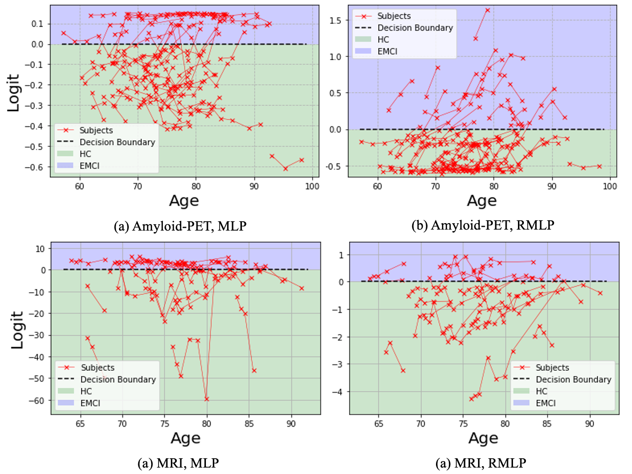
In fig. 4, we qualitatively compare the trajectories of test subjects for the task HC vs EMCI embedded by MLP (left) and RMLP(right), since they share the same structure and thereby illustrate the effectiveness of the regularization more clearly. Here we demonstrate the results from both amyloid-PET (top) and MRI (bottom) data. It can be found that although with similar performance on the accuracy, predicted risk by unregularized MLP is much more volatile across follow-up visits compared with RMLP. In particular, for subjects with multiple visits with the same diagnosis like HC or EMCI, the monotonicity of increasing risk is also preserved, suggesting the great potential of the proposed technique in modeling the subtle progression in the very early stage. The trajectories of other tasks follow the same trend, where the violation ratio is reduced similarly as shown in figs. 2 and 3.

References

- [1] Harald Hampel, John Hardy, Kaj Blennow, Christopher Chen, George Perry, Seung Hyun Kim, Victor L Villemagne, Paul Aisen, Michele Vendruscolo, Takeshi Iwatsubo, et al., “The amyloid- pathway in alzheimer’s disease,” Molecular psychiatry, vol. 26, no. 10, pp. 5481–5503, 2021.
- [2] Tong Tong, Katherine Gray, Qinquan Gao, Liang Chen, Daniel Rueckert, Alzheimer’s Disease Neuroimaging Initiative, et al., “Multi-modal classification of alzheimer’s disease using nonlinear graph fusion,” Pattern recognition, vol. 63, pp. 171–181, 2017.
- [3] Manhua Liu, Daoqiang Zhang, Dinggang Shen, Alzheimer’s Disease Neuroimaging Initiative, et al., “Ensemble sparse classification of alzheimer’s disease,” NeuroImage, vol. 60, no. 2, pp. 1106–1116, 2012.
- [4] Ahmad Wisnu Mulyadi, Wonsik Jung, Kwanseok Oh, Jee Seok Yoon, and Heung-Il Suk, “Xadlime: explainable alzheimer’s disease likelihood map estimation via clinically-guided prototype learning,” arXiv e-prints, pp. arXiv–2207, 2022.
- [5] Qi Wang, Kewei Chen, Yi Su, Eric M Reiman, Joel T Dudley, and Benjamin Readhead, “Deep learning-based brain transcriptomic signatures associated with the neuropathological and clinical severity of alzheimer’s disease,” Brain Communications, vol. 4, no. 1, pp. fcab293, 2022.
- [6] Silvia Basaia, Federica Agosta, Luca Wagner, Elisa Canu, Giuseppe Magnani, Roberto Santangelo, Massimo Filippi, Alzheimer’s Disease Neuroimaging Initiative, et al., “Automated classification of alzheimer’s disease and mild cognitive impairment using a single mri and deep neural networks,” NeuroImage: Clinical, vol. 21, pp. 101645, 2019.
- [7] Jiahong Ouyang, Qingyu Zhao, Edith V Sullivan, Adolf Pfefferbaum, Susan F Tapert, Ehsan Adeli, and Kilian M Pohl, “Longitudinal pooling & consistency regularization to model disease progression from mris,” IEEE journal of biomedical and health informatics, vol. 25, no. 6, pp. 2082–2092, 2020.
- [8] Shinya Tasaki, Jishu Xu, Denis R Avey, Lynnaun Johnson, Vladislav A Petyuk, Robert J Dawe, David A Bennett, Yanling Wang, and Chris Gaiteri, “Inferring protein expression changes from mrna in alzheimer’s dementia using deep neural networks,” Nature Communications, vol. 13, no. 1, pp. 655, 2022.
- [9] Andrew Slavin Ross, Michael C Hughes, and Finale Doshi-Velez, “Right for the right reasons: Training differentiable models by constraining their explanations,” arXiv preprint arXiv:1703.03717, 2017.
- [10] Laura Rieger, Chandan Singh, William Murdoch, and Bin Yu, “Interpretations are useful: penalizing explanations to align neural networks with prior knowledge,” in International conference on machine learning. PMLR, 2020, pp. 8116–8126.
- [11] Akhilan Boopathy, Sijia Liu, Gaoyuan Zhang, Cynthia Liu, Pin-Yu Chen, Shiyu Chang, and Luca Daniel, “Proper network interpretability helps adversarial robustness in classification,” in International Conference on Machine Learning. PMLR, 2020, pp. 1014–1023.
- [12] Yipei Wang and Xiaoqian Wang, “Self-interpretable model with transformation equivariant interpretation,” Advances in Neural Information Processing Systems, vol. 34, pp. 2359–2372, 2021.
- [13] Clifford R Jack Jr, Matt A Bernstein, Bret J Borowski, Jeffrey L Gunter, Nick C Fox, Paul M Thompson, Norbert Schuff, Gunnar Krueger, Ronald J Killiany, Charles S DeCarli, et al., “Update on the magnetic resonance imaging core of the alzheimer’s disease neuroimaging initiative,” Alzheimer’s & Dementia, vol. 6, no. 3, pp. 212–220, 2010.
- [14] Andrew J Saykin, Li Shen, Tatiana M Foroud, Steven G Potkin, Shanker Swaminathan, Sungeun Kim, Shannon L Risacher, Kwangsik Nho, Matthew J Huentelman, David W Craig, et al., “Alzheimer’s disease neuroimaging initiative biomarkers as quantitative phenotypes: Genetics core aims, progress, and plans,” Alzheimer’s & Dementia, vol. 6, no. 3, pp. 265–273, 2010.
- [15] Michael W Weiner, Dallas P Veitch, Paul S Aisen, Laurel A Beckett, Nigel J Cairns, Robert C Green, Danielle Harvey, Clifford R Jack, William Jagust, Enchi Liu, et al., “The alzheimer’s disease neuroimaging initiative: a review of papers published since its inception,” Alzheimer’s & Dementia, vol. 9, no. 5, pp. e111–e194, 2013.
- [16] Emily C Edmonds, Katherine J Bangen, Lisa Delano-Wood, Daniel A Nation, Ansgar J Furst, David P Salmon, Mark W Bondi, Alzheimer’s Disease Neuroimaging Initiative, et al., “Patterns of cortical and subcortical amyloid burden across stages of preclinical alzheimer’s disease,” Journal of the International Neuropsychological Society, vol. 22, no. 10, pp. 978–990, 2016.
- [17] Kanghan Oh, Young-Chul Chung, Ko Woon Kim, Woo-Sung Kim, and Il-Seok Oh, “Classification and visualization of alzheimer’s disease using volumetric convolutional neural network and transfer learning,” Scientific Reports, vol. 9, no. 1, pp. 1–16, 2019.
- [18] Tao Zhou, Kim-Han Thung, Xiaofeng Zhu, and Dinggang Shen, “Effective feature learning and fusion of multimodality data using stage-wise deep neural network for dementia diagnosis,” Human brain mapping, vol. 40, no. 3, pp. 1001–1016, 2019.
- [19] Zeng You, Runhao Zeng, Xiaoyong Lan, Huixia Ren, Zhiyang You, Xue Shi, Shipeng Zhao, Yi Guo, Xin Jiang, and Xiping Hu, “Alzheimer’s disease classification with a cascade neural network,” Frontiers in Public Health, vol. 8, pp. 584387, 2020.
- [20] Modupe Odusami, Rytis Maskeliūnas, Robertas Damaševičius, and Tomas Krilavičius, “Analysis of features of alzheimer’s disease: detection of early stage from functional brain changes in magnetic resonance images using a finetuned resnet18 network,” Diagnostics, vol. 11, no. 6, pp. 1071, 2021.
- [21] Ravid Shwartz-Ziv and Amitai Armon, “Tabular data: Deep learning is not all you need,” Information Fusion, vol. 81, pp. 84–90, 2022.
- [22] Tianqi Chen and Carlos Guestrin, “Xgboost: A scalable tree boosting system,” in Proceedings of the 22nd acm sigkdd international conference on knowledge discovery and data mining, 2016, pp. 785–794.
- [23] David E Rumelhart, Geoffrey E Hinton, and Ronald J Williams, “Learning internal representations by error propagation,” Tech. Rep., California Univ San Diego La Jolla Inst for Cognitive Science, 1985.
- [24] Yury Gorishniy, Ivan Rubachev, Valentin Khrulkov, and Artem Babenko, “Revisiting deep learning models for tabular data,” Advances in Neural Information Processing Systems, vol. 34, pp. 18932–18943, 2021.
- [25] Mr Amir Ebrahimighahnavieh, Suhuai Luo, and Raymond Chiong, “Deep learning to detect alzheimer’s disease from neuroimaging: A systematic literature review,” Computer methods and programs in biomedicine, vol. 187, pp. 105242, 2020.
- [26] Junhao Wen, Elina Thibeau-Sutre, Mauricio Diaz-Melo, Jorge Samper-González, Alexandre Routier, Simona Bottani, Didier Dormont, Stanley Durrleman, Ninon Burgos, Olivier Colliot, et al., “Convolutional neural networks for classification of alzheimer’s disease: Overview and reproducible evaluation,” Medical image analysis, vol. 63, pp. 101694, 2020.
- [27] Tausifa Jan Saleem, Syed Rameem Zahra, Fan Wu, Ahmed Alwakeel, Mohammed Alwakeel, Fathe Jeribi, and Mohammad Hijji, “Deep learning-based diagnosis of alzheimer’s disease,” Journal of Personalized Medicine, vol. 12, no. 5, pp. 815, 2022.