Learning the Integral Quadratic Constraints on Plant-Model Mismatch

Model-based control, with model predictive control [1] as a representative scheme, is known to be the mainstream control strategy in practice, especially for multivariable constrained control. Due to the inherent complexity of plant dynamics, the existence of disturbances and noises, as well as the expense of system identification, plant models are often far from precise, which leaves the identification of plant-model mismatch a major long-lasting issue [2, 3]. The problem of controller performance monitoring (or mismatch detection) [4, 5, 6, 7, 8] is closely related to the mismatch identification – typically, when the controller performance is found to be largely deteriorated, then mismatch needs to be characterized and compensated in the nominal model. Here, we focus on the identification problem.

From a pragmatic point of view, most model-based control schemes applied in industrial practice are linear model-based (see, e.g., [9, 10]), where transfer functions are used to represent input-output relations. Thus, we desire that plant-model mismatch is characterized in terms of the error on the nominal models in a Laplace domain. Indeed, if the plant and the nominal model can be both considered as transfer functions, then the mismatch can be identified using informative input signals with rich perturbations in the frequency range of interest [11, 12]. However, the actual plant dynamics may not be a linear one; arguably, if the plant was almost linear, then the identification of the plant model should have been accurate, making the mismatch detection and identification of less value. Thus, the plant-model mismatch is better described as one between a nonlinear plant and a linear nominal model. This can be addressed via information-theoretic [13], Gaussian process [14], or deep learning [15, 16] approaches. However, a nonlinearly described mismatch (e.g., a neural network) can be difficult to utilize in linear control, requiring significant changes or even completely replacement of the control algorithm.

Hence, we aim to characterize the underlying nonlinear plant-model mismatch “in a linear way”, so as to allow the controller design or tuning algorithm to remain in a linear framework. This is conceptually related to the classical problem of specifying the conditions for nonlinear systems to be robustly controlled by linear controllers. There exist a range of tools for this purpose, from specific to generic – absolute stability, Popov criteria, passivity, dissipativity, and integral quadratic constraint (IQC) [17]. Simply speaking, these conditions serve as “bounds” on the nonlinear non-idealities, giving rise to linear/quadratic inequalities to constrain the uncertainties and thus enabling the synthesis of robust control laws as linear ones [18, 19, 20]. In particular, the most generic characterization mentioned here, the IQC of a system, refers to the existence of dynamic multipliers on its input and output signals, such that the signal from the dynamic multipliers satisfy a quadratic dissipative inequality [21, 22, 23]. Hence, the problem of interest is how to learn the IQC on the plant-model mismatch from process input and output data.

The problem that we encounter here is similar to the ones pertaining to the learning of $L_{2}$-gain, passivity index, and dissipativity of an unknown (black-box) nonlinear system. For linear systems, these learning problems were explored based on Willems’ Fundamental Lemma [24, 25, 26]. In the author’s previous works [27, 28, 29], machine learning techniques are proposed for learning the dissipativity of nonlinear systems. A recent work from Bridgeman and her coworkers [30] gave preliminary analysis of the statistical learning theory underpinning dissipativity learning.

In this paper, we adopt the one-class support vector machine (OC-SVM) approach [27] for IQC learning and provide a generalization performance bound (similar to [30]). Specifically, in the IQC, the dynamic multiplier is fixed by choosing basis transfer functions (filters), so that the inequality specifying the IQC is parameterized by a symmetric matrix with a positive definite input diagonal block and a negative definite output diagonal block. The IQC is then expressed as linear inequality constraints involving such parameters and sampled trajectories of the plant as data. The learning of the parameters through OC-SVM yields the desired IQC characterization of the plant-model mismatch on the frequency domain.

The remaining paper is organized as follows. Preliminaries on nonlinear control theory is provided in §II. The proposed technique is then discussed in §III. A simple numerical example and a practical application are shown in §IV and §V, respectively¹¹1Codes at available at the author’s GitHub repository (https://github.com/WentaoTang-Pack/IQClearning). . Conclusions are given in §VI.

Notations. Upper case letters are used to represent matrices, transfer functions, or dynamical systems, and lower case letters are for scalars and column vectors. For a matrix $A\in\mathbb{R}^{n\times n}$ whose entries are written as $a_{ij}$ ($1\leq i,j\leq n$), its trace is $\mathrm{tr}\,A=\sum_{i=1}^{n}a_{ii}$ and its Frobenius norm is $\|A\|_{\mathrm{F}}=\left[\sum_{i=1}^{n}\sum_{j=1}^{n}|a_{ij}|^{2}\right]^{1/2}$. The inner product between two $n\times n$ matrices $A$ and $B$ is $\langle A,B\rangle:=\mathrm{tr}(A^{\top}B)=\sum_{i=1}^{n}\sum_{j=1}^{n}a_{ij}b_{ij}$. We denote by $A\succeq B$ for two symmetric matrices if $A-B$ is positive semidefinite. $I$ represents the unit matrix of appropriate dimension, or a static system where the outputs is identical to the inputs. For a complex scalar (or vector, or matrix) $a$ ($A$), we denote by $a^{\dagger}$ ($A^{\dagger}$) its conjugate (or conjugate transpose). We use $j=\sqrt{-1}$.

We consider an unknown plant dynamics (in the scope of this paper, the plant-model mismatch as a system itself) in the form of a nonlinear continuous-time system

$$\Sigma:\begin{cases}\dot{x}(t)=f(x(t),u(t))\\ y(t)=h(x(t),u(t))\end{cases}$$

defined on $t\in[0,+\infty)$, where $x(t)\in\mathbb{R}^{n_{x}}$, $u(t)\in\mathbb{R}^{n_{u}}$, and $y(t)\in\mathbb{R}^{n_{y}}$ are the states, inputs, and outputs, respectively. $f$ and $h$ are Lipschitz. We denote the Laplacian transforms of the time-domain signals by replacing $t$ with $s$ without changing the function symbol, e.g., $u(s)=\int_{0}^{\infty}u(t)e^{-st}dt$. Consider a matrix of stable proper real rational transfer functions $\Psi\in\mathcal{RH}_{\infty}^{n_{z}\times(n_{y}+n_{u})}$, called a dynamic multiplier, that act on inputs and outputs separately:

$$z(s)=\Psi(s)\begin{bmatrix}y(s)\\ u(s)\end{bmatrix}=\begin{bmatrix}\Psi_{y}(s)&0\\ 0&\Psi_{u}(s)\end{bmatrix}\begin{bmatrix}y(s)\\ u(s)\end{bmatrix}=\begin{bmatrix}z_{y}(s)\\ z_{u}(s)\end{bmatrix}.$$

When all the components of $u(\cdot)$, $y(\cdot)$ and $z(\cdot)$ are $L_{2}$-signals (square integrable on $[0,+\infty)$), a necessary condition for (1) is that it holds when $t_{1}-t_{0}\rightarrow+\infty$. According to the Parseval’s identity, this implies the following inequality, which involves a corresponding quadratic form on frequency domain integrated throughout the imaginary axis, called an integral quadratic constraint (IQC):

$$\int_{-\infty}^{+\infty}\begin{bmatrix}y^{\dagger}(j\omega)&u^{\dagger}(j\omega)\end{bmatrix}\Pi(j\omega)\begin{bmatrix}y(j\omega)\\ u(j\omega)\end{bmatrix}\geq 0,$$

(2)

where $\Pi(s)=\Psi^{\dagger}(s)M\Psi(s)$. However, (1) is defined for any $T\geq 0$. Hence, (1) is a stronger condition than (2). Therefore, (1) is also referred to as the hard IQC and (2) is called the corresponding soft IQC. $(\Psi,M)$ is said to be a hard factorization of the IQC specified by $\Pi$ [22].

Similar to the approach of [31], one can establish the following conclusion that an IQC system conforming to Definition 1 (i.e., one dissipative under a dynamic multiplier $\Psi$) should possess a storage function of the internal states. The proof is identical to the one in [31] or [28], except that $\Sigma$ should now be trivially substituted with $(\Sigma,\Psi)$.

The knowledge of IQC on the uncertainty of a system facilitates the analysis of robust stability, robust performance, and the design of the desired robust controllers (see, e.g., [21, 32]). It should, however, be pointed out that without a full model (or even with a nonlinear model), it is generally difficult to determine the IQC. Thus, in the context of identifying plant-model mismatch, we consider the problem of learning (estimating, inferring) the IQC from data.

Consider a simple case where the actual SISO system has an unknown delay not accounted for in the nominal model. The delay is $\theta\in[0,\theta_{0}]$ where the upper bound $\theta_{0}$ is known. As pointed out in [21], the plant-model mismatch $\Delta(s)=e^{-\theta s}-1$ (as a multiplicative uncertainty) satisfies IQCs of the form

$$\Pi(j\omega)=\begin{bmatrix}-\tau(j\omega)&0\\ 0&\tau(j\omega)\ell(j\omega)\end{bmatrix}$$

(6)

where $\tau(j\omega)\geq 0$ is a rational weighting function and $\ell$ is a real-valued rational function of $\omega$ satisfying $\ell(j\omega)\geq\ell_{0}(j\omega)$, in which

$$\ell_{0}(j\omega)=\max_{\theta\in[0,\theta_{0}]}|e^{-j\omega\theta}-1|^{2}=\begin{cases}4\sin^{2}\frac{\omega\theta_{0}}{2},&\omega<\pi/\theta_{0}\\ 4,&\omega\geq\pi/\theta_{0}\end{cases}.$$

Such majorization does exist, e.g., $\ell(\omega)=(4\omega^{4}+50\omega^{2})/(\omega^{4}+6.5\omega^{2}+50)$ in Megretski and Rantzer [21]. For simplicity, let $\tau\equiv 1$ be fixed and $\psi$ be learned from data. It is of interest to examine whether the learned dynamic multiplier is indeed of the theoretical form above.

Without loss of generality, say $\theta_{0}=1/2$. To generate the data, we let $u(t)$ be a sinusoidal wave $u(t)=A\sin\omega t$. Here we choose $A=1$ and $\log_{10}\omega$ is sampled from a uniform distribution on $[-2,2]$, in order to cover a sufficiently large range of frequencies. For IQC learning, $m=500$ trajectories are collected. We choose three transfer functions: $\varphi_{1}(s)=1/(s+1)$ (low-pass filter), $\varphi_{2}(s)=s/(s+1)$ (high-pass filter), and $\varphi_{3}(s)=\varphi_{1}(s)\varphi_{2}(s)$ (band-pass filter) to extract the input features, i.e., let $z_{1}=y$ and $z_{k+1}=\varphi_{k}(s)u$ ($k=1,2,3$). We aim to obtain a matrix of the form $M=\mathrm{diag}(-1,M_{u})$ where $M_{u}$ is a positive semidefinite $3\times 3$ matrix.

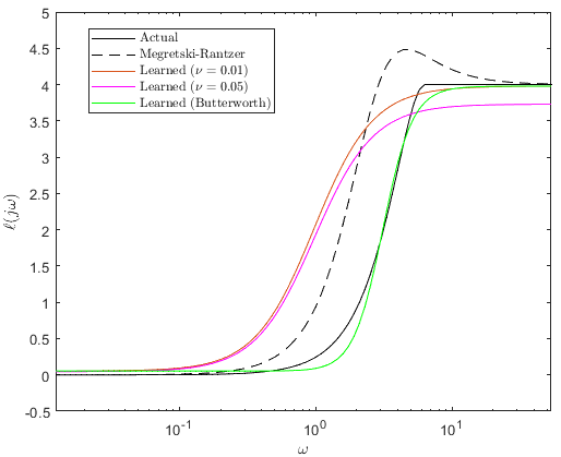
By solving the resulting optimization problem (5) in cvx (version 2.2 in Matlab R2024b), the $M$ matrix is found as

$$M=\begin{bmatrix}0.0245&-0.0120&0.0221\\ -0.0120&3.9616&0.0158\\ 0.0221&0.0158&0.0227\\ \end{bmatrix}\approx\mathrm{diag}(0,4,0)$$

which gives $\ell(j\omega)\approx 4\omega^{2}/(1+\omega^{2})$. The comparison of the learned IQC is compared with the theoretical one as well as the lowest possible curve $\ell_{0}(j\omega)$ in Fig. 2. Here the softness parameter $\nu=0.01$ is chosen, which results in a small violation of the OC-SVM margin $\sum_{i=1}^{m}\xi_{i}/m=9.34\times 10^{-4}$. When $\nu$ is increased to $0.05$, the average violation becomes $3.07\times 10^{-2}$, causing more high-frequency learning error. This indicates that OC-SVM is a suitable learning tool, at least when the dataset is clean and informative.

From the result, it is found that the learned IQC provides an approximately correct characterization of the underlying uncertainty, in the sense that except when $\omega\gtrsim\pi/\theta_{0}$, the IQC learned is an overestimation, and also upon $\omega\rightarrow 0$ and $\omega\rightarrow\infty$, the limits are close to the actual values. On the other hand, since the learned IQC dominantly relies on the high-pass features of the input to provide the S-shaped curve, the pole that is assigned to $\varphi_{2}(s)$, which is $1$, misaligns with the half-rise frequency $\pi/2\theta_{0}$ of $\ell_{0}(j\omega)$. Also, the rise of $\ell_{0}$ is steeper than a first-order high-pass filter. Hence, to attempt for a tighter estimation, we set $\varphi_{1}$ as the second Butterworth filter with cutoff frequency $\pi/2\theta_{0}$, and $\varphi_{2}$ as its high-pass counterpart. The resulting $\ell$ is shown in Fig. 2 as well. As expected, the learned IQC becomes more accurate; however, this assumes prior knowledge on a better pole assignment and better filter choice.

Empirically, we found that the learning result is insensitive to the sampling strategy in this simple example. When sampling $u(t)$ as random binary sequences (with a discretization time of $0.05$) or as truncated Fourier series with $5$ sinusoidal waves of uniformly distributed coefficients, the IQC learned remain identical to the ones shown above. Such robustness should be due to the a priori selection of a correct IQC structure (6) that relies on the user’s judgment.

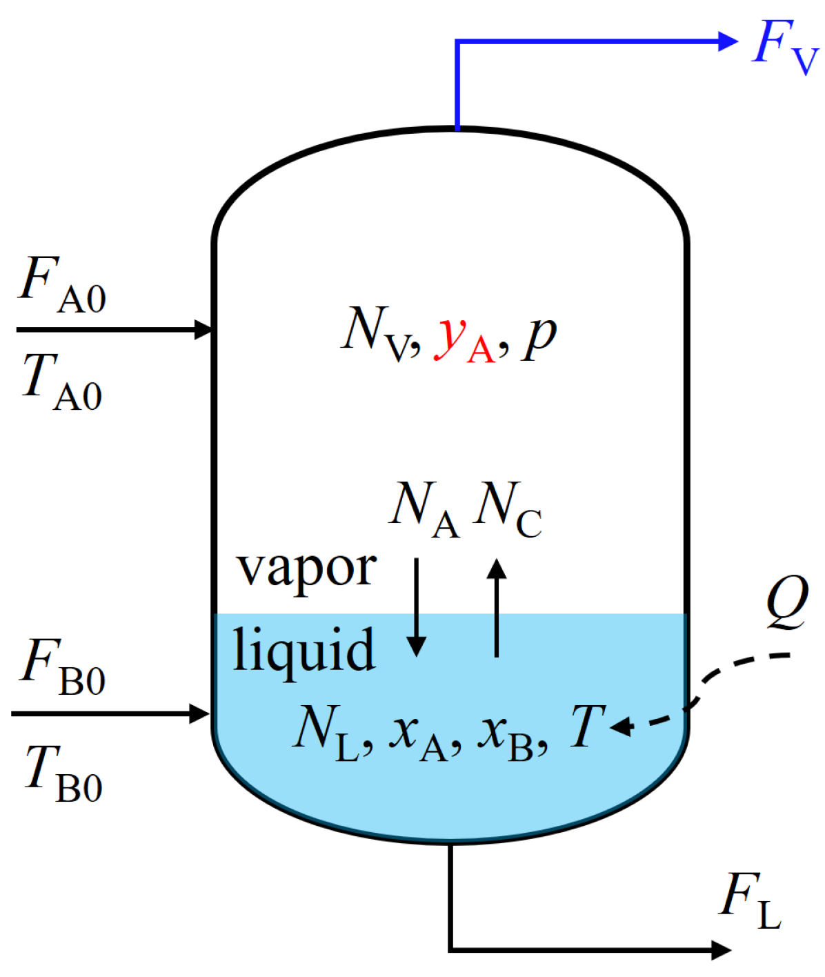
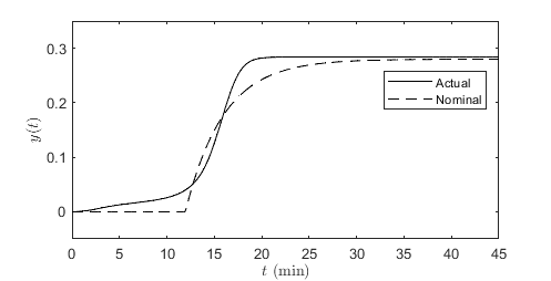
Consider the two-phase reactor in [35]. An illustration of the process is provided in Fig. 3(a) and the underlying true model, which is nonlinear, was detailed in [29]. We focus on the relation between the vapor flow rate $F_{\text{V}}$ as an input ($u$) and the substrate concentration in the vapor phase $y_{\text{A}}$ as an output ($y$). The step response of this process is shown in Fig. 3(b). Suppose that from this step response, a simplistic engineer considers the delayed first-order transfer function $\Pi_{0}(s)=K_{0}e^{-\theta_{0}s}/(\tau_{0}s+1)$ as the linear nominal model, where $K_{0}=0.28$, $\tau_{0}=4$, and $\theta_{0}=12$. The step response of the nominal model is plotted in contrast to the actual step response in Fig. 3(b). We are thus interested in characterizing the nonlinear plant-model mismatch $\Delta=\Pi-\Pi_{0}$.

We sample $m=500$ trajectories from the unknown nonlinear dynamics under input excitations $u(t)=A\sin\omega t$ for a duration of $45$ min, where $\log_{10}\omega\tau_{0}$ comes from a uniform distribution on $[-2,2]$ and $A=1/4$. Under these settings, the simulations are numerically stable. To learn the IQC, we choose the IQC structure as in (6) with $\tau(j\omega)\equiv 1$ and $M=\mathrm{diag}(1,M_{u})$. Thus, $\ell(j\omega)=\Psi_{u}(j\omega)^{\dagger}M_{u}\Psi_{u}(j\omega)$. The filters in $\Psi_{u}(s)$ are decided in the following way: (i) $9$ frequencies ($\omega_{1}=10^{-1},\omega_{2}=10^{-3/4},\cdots,\omega_{9}=10^{1}$) are first chosen; (ii) between each two frequencies $\omega_{k}$ and $\omega_{k+1}$, let $\varphi_{k}(s)=\frac{s/\omega_{k}}{s/\omega_{k}+1}\cdot\frac{1}{s/\omega_{k+1}+1}$; and (iii) let $\varphi_{0}(s)=\frac{1}{s/\omega_{1}+1}$ and $\varphi_{10}(s)=\frac{s/\omega_{9}}{s/\omega_{9}+1}$.

The resulting $\ell(\omega)$ of the learned IQC under different SVM softness parameters $\nu$, as well as when the high-pass and low-pass filters are substituted by the Butterworth second-order ones, are shown in Fig. 4. Similar to as observed in the previous section, when using simple filters, the curve of $\ell(j\omega)$ tend to be less steep, while Butterworth second-order filters better concentrate the frequency-domain uncertainties. With large $\nu$, the violation to the linear inequality constraints in the OC-SVM problem (5) can cause an erroneous high-frequency mismatch identification. It is therefore necessary to adopt a small enough $\nu$ to recover the anticipated conclusion that the mismatch should not be significant at very low or very high frequencies.

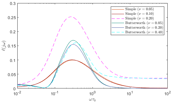
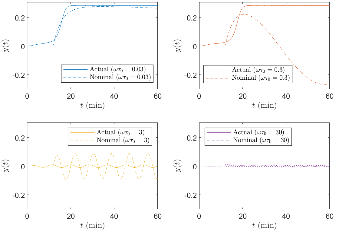
It thus appears from Fig. 4 that at a frequency $\omega\tau_{0}\approx 0.3$, the mismatch peaks. For a verification that the mismatch is indeed most severe around this frequency, we compare the actual and nominal responses under $u(t)=\cos\omega t$ for $\omega\tau_{0}=0.03,0.3,3,30$, shown in Fig. 5. One can intuitively observe here that while the nominal response is a delayed wave, the actual nonlinear dynamics does not even exhibit any oscillation for $\omega\tau_{0}=0.3$. Therefore, we conclude that the proposed IQC learning approach indeed provides an accurate description of the plant-model mismatch on the frequency domain.

In this work, a practical and efficient-to-implement approach to characterize the mismatch between a nonlinear plant and its nominal model in the form of a parameterized IQC. A numerical example and a realistic chemical process application demonstrate its capacity to accurately recover the mismatch information on the frequency domain. The IQC learned allows the synthesis of robust model-based controllers. With increasing practice of machine learning in the context of data-driven control [36], it is envisioned that the proposed method can find its use in state-of-the-art control technology. For nonlinear MPC, possible extensions of the current approach to corresponding nonlinear model structures will be studied in the future research.

The author thanks Dr. Pierre Carrette, Advanced Process Control R&D Lead at Shell Global Solutions, whom the author worked for several years ago, for the exposure to plant-model mismatch detection and identification problems.

References

- [1] J. B. Rawlings, D. Q. Mayne, and M. Diehl, Model predictive control: Theory, computation, and design. Nob Hill, 2nd ed., 2018.
- [2] P. Van den Hof, “Closed-loop issues in system identification,” Ann. Rev. Control, vol. 22, pp. 173–186, 1998.
- [3] A. S. Badwe, R. S. Patwardhan, S. L. Shah, S. C. Patwardhan, and R. D. Gudi, “Quantifying the impact of model-plant mismatch on controller performance,” J. Process Control, vol. 20, no. 4, pp. 408–425, 2010.
- [4] S. J. Qin, “Control performance monitoring – a review and assessment,” Comput. Chem. Eng., vol. 23, no. 2, pp. 173–186, 1998.
- [5] S. J. Qin and J. Yu, “Recent developments in multivariable controller performance monitoring,” J. Process Control, vol. 17, no. 3, pp. 221–227, 2007.
- [6] B. Huang and R. Kadali, Dynamic modeling, predictive control and performance monitoring: A data-driven subspace approach. Springer, 2008.
- [7] S. Kaw, A. K. Tangirala, and A. Karimi, “Improved methodology and set-point design for diagnosis of model-plant mismatch in control loops using plant-model ratio,” J. Process Control, vol. 24, no. 11, pp. 1720–1732, 2014.
- [8] X. Gao, F. Yang, C. Shang, and D. Huang, “A review of control loop monitoring and diagnosis: Prospects of controller maintenance in big data era,” Chin. J. Chem. Eng., vol. 24, no. 8, pp. 952–962, 2016.
- [9] D. M. Prett and M. Morari, The Shell process control workshop. Butterworth, 1987.
- [10] W. Tang, P. Carrette, Y. Cai, J. M. Williamson, and P. Daoutidis, “Automatic decomposition of large-scale industrial processes for distributed MPC on the Shell-Yokogawa Platform for Advanced Control and Estimation (PACE),” Comput. Chem. Eng., vol. 178, p. 108382, 2023.
- [11] A. S. Badwe, R. D. Gudi, R. S. Patwardhan, S. L. Shah, and S. C. Patwardhan, “Detection of model-plant mismatch in MPC applications,” J. Process Control, vol. 19, no. 8, pp. 1305–1313, 2009.
- [12] D. Ling, Y. Zheng, H. Zhang, W. Yang, and B. Tao, “Detection of model-plant mismatch in closed-loop control system,” J. Process Control, vol. 57, pp. 66–79, 2017.
- [13] Y. Chen and M. Ierapetritou, “A framework of hybrid model development with identification of plant-model mismatch,” AIChE J., vol. 66, no. 10, p. e16996, 2020.
- [14] Q. Wu and W. Du, “Online detection of model-plant mismatch in closed-loop systems with gaussian processes,” IEEE Trans. Ind. Inform., vol. 18, no. 4, pp. 2213–2222, 2021.
- [15] S. H. Son, J. W. Kim, T. H. Oh, D. H. Jeong, and J. M. Lee, “Learning of model-plant mismatch map via neural network modeling and its application to offset-free model predictive control,” J. Process Control, vol. 115, pp. 112–122, 2022.
- [16] F. Moayedi, A. Chandrasekar, S. Rasmussen, S. Sarna, B. Corbett, and P. Mhaskar, “Physics-informed neural networks for process systems: Handling plant-model mismatch,” Ind. Eng. Chem. Res., vol. 63, no. 31, pp. 13650–13659, 2024.
- [17] S. Sastry, Nonlinear systems: Analysis, stability, and control. Springer, 1999.
- [18] K. Zhou and J. C. Doyle, Essentials of robust control. Prentice Hall, 1998.
- [19] G. E. Dullerud and F. Paganini, A course in robust control theory: A convex approach. Springer, 2001.
- [20] R. Lozano, B. Brogliato, O. Egeland, and B. Maschke, Dissipative systems analysis and control: Theory and applications. Springer, 2013.
- [21] A. Megretski and A. Rantzer, “System analysis via integral quadratic constraints,” IEEE Trans. Autom. Control, vol. 42, no. 6, pp. 819–830, 1997.
- [22] P. Seiler, “Stability analysis with dissipation inequalities and integral quadratic constraints,” IEEE Trans. Autom. Control, vol. 60, no. 6, pp. 1704–1709, 2014.
- [23] J. Veenman, C. W. Scherer, and H. Köroğlu, “Robust stability and performance analysis based on integral quadratic constraints,” Eur. J. Control, vol. 31, pp. 1–32, 2016.
- [24] B. Wahlberg, M. B. Syberg, and H. Hjalmarsson, “Non-parametric methods for -gain estimation using iterative experiments,” Automatica, vol. 46, no. 8, pp. 1376–1381, 2010.
- [25] J. Berberich and F. Allgöwer, “A trajectory-based framework for data-driven system analysis and control,” in Eur. Control Conf. (ECC), pp. 1365–1370, IEEE, 2020.
- [26] A. Koch, J. Berberich, and F. Allgöwer, “Provably robust verification of dissipativity properties from data,” IEEE Trans. Autom. Control, vol. 67, no. 8, pp. 4248–4255, 2021.
- [27] W. Tang and P. Daoutidis, “Input-output data-driven control through dissipativity learning,” in Am. Control Conf. (ACC), pp. 4217–4222, IEEE, 2019.
- [28] W. Tang and P. Daoutidis, “Dissipativity learning control (DLC): A framework of input–output data-driven control,” Comput. Chem. Eng., vol. 130, p. 106576, 2019.
- [29] W. Tang and P. Daoutidis, “Dissipativity learning control (DLC): theoretical foundations of input–output data-driven model-free control,” Syst. Control Lett., vol. 147, p. 104831, 2021.
- [30] E. LoCicero, A. Penne, and L. Bridgeman, “Issues with input-space representation in nonlinear data-based dissipativity estimation,” arXiv preprint, 2024. arXiv:2411.13404.
- [31] D. Hill and P. Moylan, “The stability of nonlinear dissipative systems,” IEEE Trans. Autom. Control, vol. 21, no. 5, pp. 708–711, 1976.
- [32] J. Veenman and C. W. Scherer, “IQC-synthesis with general dynamic multipliers,” Int. J. Robust Nonlin. Control, vol. 24, no. 17, pp. 3027–3056, 2014.
- [33] L. Knockaert, “On orthonormal Müntz-Laguerre filters,” IEEE Trans. Signal Process., vol. 49, no. 4, pp. 790–793, 2001.
- [34] B. Schölkopf, J. C. Platt, J. Shawe-Taylor, A. J. Smola, and R. C. Williamson, “Estimating the support of a high-dimensional distribution,” Neur. Comput., vol. 13, no. 7, pp. 1443–1471, 2001.
- [35] A. Kumar and P. Daoutidis, “Feedback control of nonlinear differential-algebraic-equation systems,” AIChE J., vol. 41, no. 3, pp. 619–636, 1995.
- [36] W. Tang and P. Daoutidis, “Data-driven control: Overview and perspectives,” in Am. Control Conf. (ACC), pp. 1048–1064, IEEE, 2022.