Learning Stochastic Dynamics from Data
Abstract
We present a noise guided trajectory based system identification method for inferring the dynamical structure from observation generated by stochastic differential equations. Our method can handle various kinds of noise, including the case when the the components of the noise is correlated. Our method can also learn both the noise level and drift term together from trajectory. We present various numerical tests for showcasing the superior performance of our learning algorithm.
1 Introduction
Stochastic Differential Equation (SDE) is a fundamental modeling tool in various science and engineering fields Evans (2013); Särkkä” & Solin (2019). Compared with traditional deterministic models which often fall short in capturing the stochasticity in the nature, the significance of SDE lies in the ability to model complex systems influenced by random perturbations. Hence, SDE provides insights into the behavior of such systems under uncertainty. By incorporating a random component, typically through a Brownian motion, SDE provides a more realistic and flexible framework for simulating and predicting the behavior of these complex and dynamic systems.
We consider the models following the SDE of the following form, , where the state vector , the drift term , and the stochastic noise is a Brownian motion with covariance matrix which also depends on the state. In the field of mathematical finance, there are several SDE models that are widely used, for example, Black-Scholes Model Black & Scholes (1973) in option pricing, Vasicek Model Vasicek (1977) for analyzing interest rate dynamic and Heston Model Heston (2015) for volatility studies. Apart from the field of finance, SDE has its application in physics Coffey et al. (2004); Ebeling et al. (2008) and biology Székely & Burrage (2014); Dingli & Pacheco (2011) where SDE is used to study evolution of particles subjected to random forces and modeling physical and biological systems.
The calibration of these models is crucial for their effective application in areas like derivative pricing and asset allocation in finance, as well as in the analysis of particle systems in quantum mechanics and the study of biological system behaviors in biology. This requires the use of diverse statistical and mathematical techniques to ensure the models’ outputs align with empirical data, thereby enhancing their predictive and explanatory power. Since these SDE models have explicit function form of both drift and diffusion terms, the calibration or estimation of parameters is mostly done by minimizing the least square error between observation and model prediction Mrázek & Pospíšil (2017); Abu-Mostafa (2001). SDE has also been studied for more general cases where the drift term does not have an explicit form where it satisfies with being a vector a unknown parameters. These models can be estimated with the maximum likelihood estimator approach presented in Phillips (1972). The other approach is to obtain the likelihood function by Radon Nikodym derivative over the whole observation . Inspired by theorem in Särkkä” & Solin (2019) and the Girsanov theorem, we derive a likelihood function that incorporates state-dependent correlated noise. By utilizing such likelihood function, we are able to capture the essential structure of from data with complex noise structure.
The remainder of the paper is structured as follows, section 2 outlines the framework we use to learn the drift term and the noise level (if not state dependent), we demonstrates the effectiveness of our learning by testing it on various cases summarized in section 4 and additional examples presented in Appendix B, we conclude our paper in section 5 with a few pointers for ongoing and future developments.
2 Learning Framework
We consider the following SDE
| (1) |
where is a drift term, and represents the Brownian noise with a symmetric positive definite covariance matrix .
We consider the scenario when we are given continuous observation data in the form of for . We will find the minimizer to the following loss function
| (2) |
for ; the function space is designed to be convex and compact and it is also data-driven. This loss functional is derived from the Girsanov theorem as well as inspiration from Theorem from Särkkä” & Solin (2019).
In the case of uncorrelated noise, i.e. , where is the identity matrix and is a scalar function depends on the state, representing the noise level, 2 can be simplified to
| (3) |
Moreover, we provide three different performance measures of our estimated drift. First, if we have access to original drift function , then we will use the following error to compute the difference between (our estimator) to with the following norm
| (4) |
Here the weighted measure is defined on , where it defines the region of explored due to the dynamics defined by equation 1; therefore is given as follows
| (5) |
The norm given by equation 4 is useful only from the theoretical perspective, i.e. showing convergence. In real life situation, is most likely non-accessible. Hence we will look at a performance measure that compare the difference between (the observed trajectory evolves from with the unknown ) and (the estimated trajectory evolves from the same with the learned and the same random noise as used by the original dynamics). Then, the difference between the two trajectories is measured as follows
| (6) |
However, comparing two sets of trajectories (even with the same initial condition) on the same random noise is not realistic. We compare the distribution of the trajectories over different initial conditions and all possible noise at some chosen time snapshots using the Wasserstein distance.
3 Comparison to Others
When the noise level becomes a constant, i.e. , we end up a much simpler loss
which has been investigated in Lu et al. (2022). System identification of the drift term has been studied in many different scenarios, e.g. identification by enforcing sparsity such as SINDy Brunton et al. (2016), neural network based methods such as NeuralODE Chen et al. (2018) and PINN Raissi et al. (2019), regression based Cucker & Smale (2002), and high-dimensional reduction framework Lu et al. (2019). The uniqueness of our method is that we incorporate the covariance matrix into the learning and hence improving the estimation especially when the noise is correlated.
4 Examples
In this section, we demonstrate the application of our trajectory-based method for estimating drift functions, showcasing a variety of examples. We explore drift functions ranging from polynomials in one and two dimensions to combinations of polynomials and trigonometric functions, as well as a deep learning approach in one dimension. The observations, serving as the input dataset for testing our method, are generated by the Euler-Maruyama scheme, utilizing the drift functions as we just mentioned. The basis space is constructed employing either B-spline or piecewise polynomial methods for maximum degree p-max equals . For higher order dimensions where , each basis function is derived through a tensor grid product, utilizing one-dimensional basis defined by knots that segment the domain in each dimension. The parameters for the following examples are listed in table 1. Due to space constraints, additional examples are provided in appendix B.
The estimation results are evaluated using several different metrics. We record the noise terms, , from the trajectory generation process and compare the trajectories produced by the estimated drift functions, , under identical noise conditions. We examine trajectory-wise errors using equation 6 with relative trajectory error and plot both and to calculate the relative error using 4, where is derived by 5. Additionally, we assess the distribution-wise discrepancies between observed and estimated results, computing the Wasserstein distance at various time steps.
| Simulation Scheme | Euler-Maruyama | ||
| 1 | 0.6 | ||
| 0.001 | |||
| Uniform(0,10) | 10000 | ||
| p-max | 2 | Basis Type | B-Spline / PW-Polynomial |
4.1 Example: sine/cosine drift
We initiate our numerical study with a one-dimensional () drift function that incorporates both polynomial and trigonometric components, given by .
Figure 1 illustrates the comparison between the true drift function and the estimated drift function , alongside a comparison of trajectories. Notably, Figure 1(a) on the left includes a background region depicting the histogram of , which represents the distribution of observations over the domain of . This visualization reveals that in regions where has a higher density of observations—indicated by higher histogram values—the estimation of tends to be more accurate. Conversely, in less dense regions of the dataset (two ends of the domain), the estimation accuracy of diminishes.
Table 2 presents a detailed quantitative analysis of the estimation results, including the norm difference between and , as well as the trajectory error. Furthermore, the table compares the distributional distances between and at selected time steps, with the Wasserstein distance results included.

| Number of Basis | 8 | Wasserstein Distance | |
|---|---|---|---|
| Maximum Degree | 2 | 0.0291 | |
| Relative Error | 0.007935 | 0.0319 | |
| Relative Trajectory Error | 0.0020239 0.002046 | 0.0403 | |
4.2 Example: Deep Neural Networks
We continue our numerical investigation with a one-dimensional () drift function which is given by . Figure 2 illustrates the comparison between the true drift function and the estimated drift function , alongside a comparison of trajectories. Recall the setup of figures are similar to the ones presented in previous section.

The error for learning turns out to be bigger, especially towards the two end points of the interval. However, the errors happen mostly during the two end points of the data interval, where the distribution of the data appears to be small, i.e. few data present in the learning. We are able to recover most the trajectory.
5 Conclusion
We have presented a novel approach of learning the drift and diffusion from a noise-guide likelihood function. Such learning can handle general noise structure as long as the covariance information of the noise is known. Unknown noise structure when the covariance is a simple scalar is still learnable through quadratic variation. However learning state-dependent covariance noise is ongoing. Testing on high-dimensional drift term is ongoing. Our loss only incorporates likelihood on the observation data. It is possible to add various penalty terms to enhance the model performance, such as the sparsity assumption enforced in SINDy and other related deep learning methods such as NeuralODE and PINN.
Acknowledgments
ZG developed the algorithm, analyzed the data and implemented the software package. ZG develops the theory with IC and MZ. MZ designed the research. All authors wrote the manuscript. MZ is partially supported by NSF- and the startup fund provided by Illinois Tech.
References
- Abu-Mostafa (2001) Y.S. Abu-Mostafa. Financial model calibration using consistency hints. IEEE Transactions on Neural Networks, 12(4):791–808, 2001. doi: 10.1109/72.935092.
- Black & Scholes (1973) Fischer Black and Myron Scholes. The pricing of options and corporate liabilities. Journal of Political Economy, 81(3):637–654, 1973. ISSN 00223808, 1537534X. URL http://www.jstor.org/stable/1831029.
- Brunton et al. (2016) S. L. Brunton, J. L. Proctor, and N. Kutz. Discovering governing equations from data by sparse identification of nonlinear dynamical systems. PNAS, 113(15):3932 – 3937, 2016.
- Chen et al. (2018) Ricky T. Q. Chen, Yulia Rubanova, Jesse Bettencourt, and David K Duvenaud. Neural ordinary differential equations. In S. Bengio, H. Wallach, H. Larochelle, K. Grauman, N. Cesa-Bianchi, and R. Garnett (eds.), Advances in Neural Information Processing Systems, volume 31. Curran Associates, Inc., 2018. URL https://proceedings.neurips.cc/paper_files/paper/2018/file/69386f6bb1dfed68692a24c8686939b9-Paper.pdf.
- Coffey et al. (2004) William Coffey, Yuri Kalmykov, and John Waldron. The Langevin Equation: With Applications to Stochastic Problems in Physics, Chemistry and Electrical Engineering. 09 2004. ISBN 978-981-238-462-1. doi: 10.1142/9789812795090.
- Cucker & Smale (2002) Felipe Cucker and Steve Smale. On the mathematical foundations of learning. Bulletin of the American mathematical society, 39(1):1–49, 2002.
- Dingli & Pacheco (2011) D. Dingli and J.M. Pacheco. Stochastic dynamics and the evolution of mutations in stem cells. BMC Biol, 9:41, 2011.
- Ebeling et al. (2008) Werner Ebeling, Ewa Gudowska-Nowak, and Igor M. Sokolov. On Stochastic Dynamics in PHysics - Remarks on History and Terminology. Acta Physica Polonica B, 39(5):1003 – 1018, 2008.
- Evans (2013) Lawrence C. Evans. An Introduction to Stochastic Differential Equations. American Mathematical Society, 2013.
- Heston (2015) Steven L. Heston. A Closed-Form Solution for Options with Stochastic Volatility with Applications to Bond and Currency Options. The Review of Financial Studies, 6(2):327–343, 04 2015. ISSN 0893-9454. doi: 10.1093/rfs/6.2.327. URL https://doi.org/10.1093/rfs/6.2.327.
- Lu et al. (2019) Fei Lu, Ming Zhong, Sui Tang, and Mauro Maggioni. Nonparametric inference of interaction laws in systems of agents from trajectory data. Proceedings of the National Academy of Sciences, 116(29):14424–14433, 2019.
- Lu et al. (2022) Fei Lu, Maruo Maggioni, and Sui Tang. Learning interaction kernels in stochastic systems of interacting particles from multiple trajectories. Foundations of Computational Mathematics, 22:1013 – 1067, 2022.
- Mrázek & Pospíšil (2017) Milan Mrázek and Jan Pospíšil. Calibration and simulation of heston model. Open Mathematics, 15(1):679–704, 2017. doi: doi:10.1515/math-2017-0058. URL https://doi.org/10.1515/math-2017-0058.
- Phillips (1972) P. C. B. Phillips. The structural estimation of a stochastic differential equation system. Econometrica, 40(6):1021–1041, 1972. ISSN 00129682, 14680262. URL http://www.jstor.org/stable/1913853.
- Raissi et al. (2019) M. Raissi, P. Perdikaris, and G.E. Karniadakis. Physics-informed neural networks: A deep learning framework for solving forward and inverse problems involving nonlinear partial differential equations. Journal of Computational Physics, 378:686–707, 2019. ISSN 0021-9991. doi: https://doi.org/10.1016/j.jcp.2018.10.045. URL https://www.sciencedirect.com/science/article/pii/S0021999118307125.
- Särkkä” & Solin (2019) Simo Särkkä” and Arno Solin. Applied Stochastic Differential Equations. Institute of Mathematical Statistics Textbooks. Cambridge University Press, 2019.
- Székely & Burrage (2014) Tamás Székely and Kevin Burrage. Stochastic simulation in systems biology. Computational and Structural Biotechnology Journal, 12(20):14–25, 2014. ISSN 2001-0370. doi: https://doi.org/10.1016/j.csbj.2014.10.003. URL https://www.sciencedirect.com/science/article/pii/S2001037014000403.
- Vasicek (1977) Oldrich Vasicek. An equilibrium characterization of the term structure. Journal of Financial Economics, 5(2):177–188, 1977. ISSN 0304-405X. doi: https://doi.org/10.1016/0304-405X(77)90016-2. URL https://www.sciencedirect.com/science/article/pii/0304405X77900162.
Appendix A Implementation
In this section, we will discuss in details how the algorithm is implemented for our learning framework presented in section 2. In real applications, continuous data is rarely obtainable, we will have to deal with discrete observation data, i.e. with being i.i.d sample from , where and . We use a discretized version of 2,
| (7) | ||||
for . Moreover, we also assume that is a finite-dimensional function space, i.e. . Then for any , , where is a constant vector coefficient and is a basis of and the domain is constructed by finding out the of the components of for . We consider two scenarios for constructing , one is to use pre-determined basis such as piecewise polynomials, Clamped B-spline, Fourier basis, or a mixture of all of the aforementioned ones; the other is to use neural networks, where the basis functions are also trained from data. Next, we can put the basis representation of back to equation 7, we obtain the following loss based on the coefficients
| (8) | ||||
In the case of covariance matrix being a diagonal matrix, i.e.
Then equation 8 can be re-written as
Here is the component of any vector . We define , and as
and as
Then equation 8 can be re-written as
Since each is decoupled from each other, we just need to solve simultaneously
Then we can obtain . However when does not have a diagonal structure, we will have to resolve to gradient descent methods to minimize equation 8 in order to find the coefficients for a total number of parameters. However, if a data-driven basis is desired, then we set to be the space neural networks with the same depth, same number of neurons and same activation functions on the hidden layers. Furthermore, we find from minimizing equation 7 using any deep learning optimizer such as Stochastic Gradient Descent or Adam from well-known deep learning packages.
Appendix B Additional Examples
For , we also worked on polynomial drift function . The estimation results are depicted in 3 and detailed in Table 3.

| Number of Basis | 10 | Wasserstein Distance | |
|---|---|---|---|
| Maximum Degree | 2 | 0.0153 | |
| Relative Error | 0.0087649 | 0.0154 | |
| Relative Trajectory Error | 0.00199719 0.00682781 | 0.0278 | |
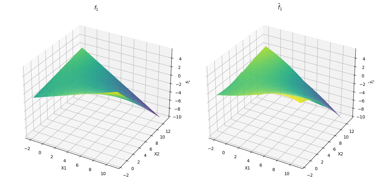
For , we examine two types of drift function : polynomial and trigonometric. Denote
where and for .
For polynomial drift function , we set
Figure 4, Figure 5(a), 5(b) and Table 4 shows evaluation of the polynomial drift function estimation result.
For trigonometric drift function , we set
Figure 6, Figure 7(a), 7(b) and Table 5 shows evaluation of the trigonometric drift function estimation result.


| Number of Basis | 36 | Wasserstein Distance | |
|---|---|---|---|
| Maximum Degree | 2 | 0.0891 | |
| Relative Error | 0.02118531 | 0.0872 | |
| Relative Trajectory Error | 0.00306613 0.00375144 | 0.0853 | |


| Number of Basis | 36 | Wasserstein Distance | |
|---|---|---|---|
| Maximum Degree | 2 | 0.1011 | |
| Relative Error | 0.02734505 | 0.1119 | |
| Relative Trajectory Error | 0.0041613 0.0079917 | 0.1293 | |