Learning Sparse Fixed-Structure Gaussian Bayesian Networks

Arnab Bhattcharyya
National University of Singapore
[email protected] Davin Choo
National University of Singapore
[email protected] Rishikesh Gajjala
Indian Institute of Science, Bangalore
[email protected] Sutanu Gayen
National University of Singapore
[email protected] Yuhao Wang
National University of Singapore
[email protected]

Abstract

Gaussian Bayesian networks (a.k.a. linear Gaussian structural equation models) are widely used to model causal interactions among continuous variables. In this work, we study the problem of learning a fixed-structure Gaussian Bayesian network up to a bounded error in total variation distance. We analyze the commonly used node-wise least squares regression LeastSquares and prove that it has the near-optimal sample complexity. We also study a couple of new algorithms for the problem:

•

BatchAvgLeastSquares takes the average of several batches of least squares solutions at each node, so that one can interpolate between the batch size and the number of batches. We show that BatchAvgLeastSquares also has near-optimal sample complexity.
•

CauchyEst takes the median of solutions to several batches of linear systems at each node. We show that the algorithm specialized to polytrees, CauchyEstTree, has near-optimal sample complexity.

Experimentally¹¹1Code is available at https://github.com/YohannaWANG/CauchyEst, we show that for uncontaminated, realizable data, the LeastSquares algorithm performs best, but in the presence of contamination or DAG misspecification, CauchyEst/CauchyEstTree and BatchAvgLeastSquares respectively perform better.

1 Introduction

Linear structural equation models (SEMs) are widely used to model interactions among multiple variables, and they have found applications in diverse areas, including economics, genetics, sociology, psychology and education; see [Mue99, Mul09] for pointers to the extensive literature in this area. Gaussian Bayesian networks are a popularly used form of SEMs where: (i) there are no hidden/unobserved variables, (ii) each variable is a linear combination of its parents plus a Gaussian noise term, and (iii) all noise terms are independent. The structure of a Bayesian network refers to the directed acyclic graph (DAG) that prescribes the parent nodes for each node in the graph.

This work studies the task of learning a Gaussian Bayesian network given its structure. The problem is obviously quite fundamental and has been subject to extensive prior work. The usual formulation of this problem is in terms of parameter estimation, where one wants a consistent estimator that exactly recovers the parameters of the Bayesian network in the limit, as the the number of samples approaches infinity. In contrast, we consider the problem from the viewpoint of distribution learning [KMR⁺94]. Analogous to Valiant’s famous PAC model for learning Boolean functions [Val84], the goal here is to learn, with high probability, a distribution $\widehat{\mathcal{P}}$ that is close to the ground-truth distribution $\mathcal{P}$ , using an efficient algorithm. In this setting, pointwise convergence of the parameters is no longer a requirement; the aim is rather to approximately learn the induced distribution. Indeed, this relaxed objective may be achievable when the former may not be (e.g., for ill-conditioned systems) and can be the more relevant requirement for downstream inference tasks. Diakonikolas [Dia16] surveys the current state-of-the-art in distribution learning from an algorithmic perspective.

Consider a Gaussian Bayesian network $\mathcal{P}$ with $n$ variables with parameters in the form of coefficients²²2We write $i\leftarrow j$ to emphasize that $X_{j}$ is the parent of $X_{i}$ in the Bayesian network. $a_{i\leftarrow j}$ ’s and variances $\sigma_{i}$ ’s. For each $i\in[n]$ , the linear structural equation for variable $X_{i}$ , with parent indices $\pi_{i}\subseteq[n]$ , is as follows:

X_{i}=\eta_{i}+\sum_{j\in\pi_{i}}a_{i\leftarrow j}X_{j},\qquad\eta_{i}\sim N(0,\sigma_{i}^{2})

for some unknown parameters $a_{i\leftarrow j}$ ’s and $\sigma_{i}$ ’s. If a variable $X_{i}$ has no parents, then $X_{i}\sim N(0,\sigma_{i}^{2})$ is simply an independent Gaussian. Our goal is to efficiently learn a distribution $\mathcal{Q}$ such that

\mathrm{d_{TV}}(\mathcal{P},\mathcal{Q})\leq\varepsilon

while minimizing the number of samples we draw from $\mathcal{P}$ as a function of $n$ , $\varepsilon$ and relevant structure parameters. Here, $\mathrm{d_{TV}}$ denotes the total variation or statistical distance between two distributions:

\mathrm{d_{TV}}(\mathcal{P},\mathcal{Q})=\frac{1}{2}\int_{\mathbb{R}^{n}}\left\lvert\mathcal{P}(x)-\mathcal{Q}(x)\right\rvert dx.

One way to approach the problem is to simply view $\mathcal{P}$ as an $n$ -dimensional multivariate Gaussian. In this case, it is known that the Gaussian $\mathcal{Q}\sim N(0,\widehat{\Sigma})$ defined by the empirical covariance matrix $\widehat{\Sigma}$ , computed with $\mathcal{O}(n^{2}/\varepsilon^{2})$ samples from $\mathcal{P}$ , is $\varepsilon$ -close in TV distance to $\mathcal{P}$ with constant probability [ABDH⁺20, Appendix C]. This sample complexity is also necessary for learning general $n$ -dimensional Gaussians and hence general Gaussian Bayesian networks on $n$ variables.

We focus therefore on the setting where the structure of the network is sparse.

Assumption 1.1.

Each variable in the Bayesian network has at most $d$ parents. i.e. $\left\lvert\pi_{i}\right\rvert\leq d,\forall i\in[n]$ .

Sparsity is a common and very useful assumption for statistical learning problems; see the book [HTW19] for an overview of the role of sparsity in regression. More specifically, in our context, the assumption of bounded in-degree is popular (e.g., see [Das97, BCD20]) and also very natural, as it reflects the belief that in the correct model, each linear structural equation involves a small number of variables³³3More generally, one would want to assume a bound on the “complexity” of each equation. In our context, as each equation is linear, the complexity is simply proportional to the in-degree..

1.1 Our contributions

1.

Analysis of MLE LeastSquares and a distributed-friendly generalization BatchAvgLeastSquares

The standard algorithm for parameter estimation of Gaussian Bayesian networks is to perform node-wise least squares regression. It is easy to see that LeastSquares is the maximum likelihood estimator. However, to the best of our knowledge, there did not exist an explicit sample complexity bound for this estimator. We show that the sample complexity for learning $\mathcal{P}$ to within TV distance $\varepsilon$ using LeastSquares requires only $\widetilde{\mathcal{O}}(nd/\varepsilon^{2})$ samples, which is nearly optimal.

We also give a generalization dubbed BatchAvgLeastSquares which solves multiple batches of least squares problems (on smaller systems of equations), and then returns their mean. As each batch is independent from the others, they can be solved separately before their solutions are combined. Our analysis will later show that we can essentially interpolate between “batch size” and “number of batches” while maintaining a similar total sample complexity – LeastSquares is the special case of a single batch. Notably, we do not require any additional assumptions about the coefficients or variance terms in the analyses of LeastSquares and BatchAvgLeastSquares.
2.

New algorithms based on Cauchy random variables: CauchyEst and CauchyEstTree

We develop a new algorithm CauchyEst. At each node, CauchyEst solves several small linear systems of equations and takes the component-wise median of the obtained solution to obtain an estimate of the coefficients for the corresponding structural equation. In the special case of bounded-degree polytree structures, where the underlying undirected Bayesian network is acyclic, we specialize the algorithm to CauchyEstTree for which we give theoretical guarantees. Polytrees are of particular interest because inference on polytree-structured Bayesian networks can be performed efficiently [KP83, Pea86]. On polytrees, we show that the sample complexity of CauchyEstTree is also $\widetilde{\mathcal{O}}(nd/\varepsilon^{2})$ . Somewhat surprisingly, our analysis (as the name of the algorithm reflects) involves Cauchy random variables which usually do not arise in the context of regression.
3.

Hardness results

In Section 5, we show that our sample complexity upper-bound is nearly optimal in terms of the dependence on the parameters $n$ , $d$ , and $\epsilon$ . In particular, we show that learning the coefficients and noises of a linear structural equation model (on $n$ variables, with in-degree at most $d$ ) up to an $\epsilon$ -error in $\mathrm{d_{TV}}$ -distance with probability 2/3 requires $\Omega(nd\epsilon^{-2})$ samples in general. We use a packing argument based on Fano’s inequality to achieve this result.
4.

Extensive experiments on synthetic and real-world networks

We experimentally compare the algorithms studied here as well as other well-known methods for undirected Gaussian graphical model regression, and investigate how the distance between the true and learned distributions changes with the number of samples. We find that the LeastSquares estimator performs the best among all algorithms on uncontaminated datasets. However, CauchyEst, CauchyEstTree and BatchMedLeastSquares outperform LeastSquares and BatchAvgLeastSquares by a large margin when a fraction of the samples are contaminated. In non-realizable/agnostic learning case, BatchAvgLeastSquares, CauchyEst, and CauchyEstTree performs better than the other algorithms.

1.2 Outline of paper

In Section 2, we relate KL divergence with TV distance and explain how to decompose the KL divergence into $n$ terms so that it suffices for us to estimate the parameters for each variable independently. We also give an overview of our two-phased recovery approach and explain how to use recovered coefficients to estimate the variances via VarianceRecovery. For estimating coefficients, Section 3 covers the estimators based on linear least squares (LeastSquares and BatchAvgLeastSquares) while Section 4 presents our new Cauchy-based algorithms (CauchyEst and CauchyEstTree). To complement our algorithmic results, we provide hardness results in Section 5 and experimental evaluation in Section 6.

For a cleaner exposition, we defer some formal proofs to Appendix B.

1.3 Further related work

Bayesian networks, both in discrete and continuous settings, were formally introduced by Pearl [Pea88] in 1988 to model uncertainty in AI systems. For the continuous case, Pearl considered the case when each node is a linear function of its parents added with an independent Gaussian noise [Pea88, Chapter 7]. The parameter learning problem – recovering the distribution of nodes conditioned on its parents from data – is well-studied in practice, and maximum likelihood estimators are known for various simple settings such as when the conditional distribution is Gaussian or the variables are discrete-valued. See for example the implementation of fit in the R package bnlearn [Scu20].

The focus of our paper is to give formal guarantees for the parameter learning in the PAC framework introduced by Valiant [Val84] in 1984. Subsequently, Haussler [Hau18] generalized this framework for studying parameter and density estimation problems of continuous distributions. Dasgupta [Das97] first looked at the problem of parameter learning for fixed structure Bayesian networks in the discrete and continuous settings and gave finite sample complexity bounds for these problems based on the VC-dimensions of the hypothesis classes. In particular, he gave an algorithm for learning the parameters of a Bayes net on $n$ binary variables of bounded in-degree in $\mathrm{d_{KL}}$ distance using a quadratic in $n$ samples. Subsequently, tight (linear) sample complexity upper and lower bounds were shown for this problem [BGMV20, BGPV20, CDKS20]. To the best of our knowledge, a finite PAC-style bound for fixed-structure Gaussian Bayesian networks was not known previously.

The question of structure learning for Gaussian Bayesian networks has been extensively studied. A number of works [PB14, GH17, CDW19, PK20, Par20, GDA20] have proposed increasingly general conditions for ensuring identifiability of the network structure from observations. Structure learning algorithms that work for high-dimensional Gaussian Bayesian networks have also been proposed by others (e.g., see [AZ15, AGZ19, GZ20]).

2 Preliminaries

In this section, we discuss why we upper bound the total variational distance using KL divergence and give a decomposition of the KL divergence into $n$ terms, one associated with each variable in the Bayesian network. This decomposition motivates why our algorithms and analysis focus on recovering parameters for a single variable. We also present our general two-phased recovery approach and explain how to estimate variances using recovered coefficients in Section 2.6.

2.1 Notation

A Bayesian network (Bayes net in short) $\mathcal{P}$ is a joint distribution $\mathcal{P}$ over $n$ variables $X_{1},\ldots,X_{n}$ defined by the underlying directed acyclic graph (DAG) $G$ . The DAG $G=(V,E)$ encodes the dependence between the variables where $V=\left\{X_{1},\ldots,X_{n}\right\}$ and $(X_{j},X_{i})\in E$ if and only if $X_{j}$ is a parent of $X_{i}$ . For any variable $X_{i}$ , we use the set $\pi_{i}\subseteq[n]$ to represent the indices of $X_{i}$ ’s parents. Under this notation, each variable $X_{i}$ of $\mathcal{P}$ is independent of $X_{i}$ ’s non-descendants conditioned on $\pi_{i}$ . Therefore, using Bayes rule in the topological order of $G$ , we have

\mathcal{P}(X_{1},\ldots,X_{n})=\prod_{i=1}^{n}\Pr_{\mathcal{P}}(X_{i}\mid\pi_{i})

Without loss of generality, by renaming variables, we may assume that each variable $X_{i}$ only has ancestors with indices smaller than $i$ . We also define $p_{i}=\left\lvert\pi_{i}\right\rvert$ as the number of parents of $X_{i}$ and $d_{avg}=\frac{1}{n}\sum_{i=1}^{n}p_{i}$ to be average in-degree. Furthermore, a DAG $G$ is a polytree if the undirected version of $G$ is a acyclic.

We study the realizable setting where our unknown probability distribution $\mathcal{P}$ is Markov with respect to the given Bayesian network. We denote the true (hidden) parameters associated with $\mathcal{P}$ by $\alpha^{*}=(\alpha^{*}_{1},\ldots,\alpha^{*}_{n})$ . Our algorithms recover parameter estimates $\widehat{\alpha}=(\widehat{\alpha}_{1},\ldots,\widehat{\alpha}_{n})$ such that the induced probability distribution $\mathcal{Q}$ is close in total variational distance to $\mathcal{P}$ . For each $i\in[n]$ , $\alpha_{i}^{*}=(A_{i},\sigma_{i})$ is the set of ground truth parameters associated with variable $X_{i}$ , $A_{i}$ is the coefficients associated to $\pi_{i}$ , $\sigma_{i}^{2}$ is the variance of $\eta_{i}$ , $\widehat{\alpha}_{i}^{*}=(\widehat{A}_{i},\widehat{\sigma}_{i})$ is our estimate of $\alpha_{i}^{*}$ .

In the course of the paper, we will often focus on the perspective a single variable of interest. This allows us to drop a subscript for a cleaner discussion. Let us denote such a variable of interest by $Y\in V$ and use the index $y\in[n]$ . Without loss of generality, by renaming variables, we may further assume that the parents of $Y$ are $X_{1},\ldots,X_{p}$ . By 1.1, we know that $p\leq d$ . We can write $Y=\eta_{y}+\sum_{i=1}^{p}a_{y\leftarrow i}X_{i}$ where $\eta_{y}\sim N(0,\sigma_{y}^{2})$ . We use matrix $M\in\mathbb{R}^{p\times p}$ to denote the covariance matrix defined by the parents of $Y$ , where $M_{i,j}=\mathbb{E}\left[X_{i}X_{j}\right]$ and $M=LL^{\top}$ is the Cholesky decomposition of $M$ . Under this notation, we see the vector $(X_{1},\ldots,X_{p})\sim N(0,M)$ is distributed as a multivariate Gaussian. Our goal is then to produce estimates $\widehat{a}_{y\leftarrow i}$ for each $a_{y\leftarrow i}$ . For notational convenience, we can group the coefficients into $A=\left[a_{y\leftarrow 1},\ldots,a_{y\leftarrow p}\right]^{\top}$ and $\widehat{A}=\left[\widehat{a}_{y\leftarrow 1},\ldots,\widehat{a}_{y\leftarrow p}\right]^{\top}$ . The vector $\Delta=(\widehat{A}-A)^{\top}$ captures the entry-wise gap between our estimates and the ground truth.

We write $[n]$ to mean $\{1,2,\ldots,n\}$ and $\left\lvert S\right\rvert$ to mean the size of a set $S$ . For a matrix $M$ , $M_{i,j}$ denotes its $(i,j)$ -th entry. We use $\left\lVert\cdot\right\rVert$ to both mean the operator/spectral norm for matrices and $L_{2}$ -norm for vectors, which should be clear from context. We hide absolute constant multiplicative factors and multiplicative factors poly-logarithmic in the argument using standard notations: $\mathcal{O}(\cdot)$ , $\Omega(\cdot)$ , and $\widetilde{\mathcal{O}}(\cdot)$ .

2.2 Basic facts and results

We begin by stating some standard facts and results.

Fact 2.1.

Suppose $X\sim N(0,\sigma^{2})$ . Then, for any $t>0$ , $\Pr\left(X>t\right)\leq\exp\left(-\frac{t^{2}}{2\sigma^{2}}\right)$ .

Fact 2.2.

Consider any matrix $B\in\mathbb{R}^{n\times m}$ with rows $B_{1},\ldots,B_{n}\in\mathbb{R}^{m}$ . For any $i\in[m]$ and any vector $v\in\mathbb{R}^{m}$ with i.i.d. $N(0,\sigma^{2})$ entries, we have that $(Bv)_{i}=B_{i}v\sim N(0,\sigma^{2}\cdot\left\lVert B_{i}\right\rVert^{2})$ .

Fact 2.3 (Theorem 2.2 in [Gut09])).

Let $X_{1},\ldots,X_{p}\sim N(0,LL^{\top})$ be $p$ i.i.d. $n$ -dimensional multivariate Gaussians with covariance $LL^{\top}\in\mathbb{R}^{n\times n}$ (i.e. $L\in\mathbb{R}^{n\times p}$ ). If $X\in\mathbb{R}^{p\times n}$ is the matrix formed by stacking $X_{1},\ldots,X_{p}$ as rows of $X$ , then $X=GL^{\top}$ where $G\in\mathbb{R}^{p\times p}$ is a random matrix with i.i.d. $N(0,1)$ entries.⁴⁴4The transformation stated in [Gut09, Theorem 2.2, page 120] is for a single multivariate Gaussian vector, thus we need to take the transpose when we stack them in rows. Note that $G$ and $G^{\top}$ are identically distributed.

Lemma 2.4 (Equation 2.19 in [Wai19]).

Let $Y=\sum_{k=1}^{n}Z_{k}^{2}$ , where each $Z_{k}\sim N(0,1)$ . Then, $Y\sim\chi^{2}_{n}$ and for any $0<t<1$ , we have $\Pr\left(\left\lvert Y/n-1\right\rvert\geq t\right)\leq 2\exp\left(-nt^{2}/8\right)$ .

Lemma 2.5 (Consequence of Corollary 3.11 in [BVH⁺16]).

Let $G\in\mathbb{R}^{n\times m}$ be a matrix with i.i.d. $N(0,1)$ entries where $n\leq m$ . Then, for some universal constant $C$ , $\Pr\left(\left\lVert G\right\rVert\geq 2(\sqrt{n}+\sqrt{m})\right)\leq\sqrt{n}\cdot\exp\left(-C\cdot m\right)$ .

Lemma 2.6.

Let $G\in\mathbb{R}^{k\times d}$ be a matrix with i.i.d. $N(0,1)$ entries. Then, for any constant $0<c_{1}<1/2$ and $k\geq d/c_{1}^{2}$ ,

\Pr\left(\left\lVert(G^{\top}G)^{-1}\right\rVert_{op}\leq\frac{1}{\left(1-2c_{1}\right)^{2}k}\right)\geq 1-\exp\left(-\frac{kc_{1}^{2}}{2}\right)

Proof.

See Appendix B. ∎

Lemma 2.7.

Let $G\in\mathbb{R}^{k\times p}$ be a matrix with i.i.d. $N(0,1)$ entries and $\eta\in\mathbb{R}^{k}$ be a vector with i.i.d. $N(0,\sigma^{2})$ entries, where $G$ and $\eta$ are independent. Then, for any constant $c_{2}>0$ ,

\Pr\left(\left\lVert G^{\top}\eta\right\rVert_{2}<2\sigma c_{2}\sqrt{kp}\right)\geq 1-2p\exp\left(-2k\right)-p\exp\left(-\frac{c_{2}^{2}}{2}\right)

Proof.

See Appendix B. ∎

The next result gives the non-asymptotic convergence of medians of Cauchy random variables. We use this result in the analysis of CauchyEst, and it may be of independent interest.

Lemma 2.8.

[Non-asymptotic convergence of Cauchy median] Consider a collection of $m$ i.i.d. $\mathrm{Cauchy}(0,1)$ random variables $X_{1},\ldots,X_{m}$ . Given a threshold $0<\tau<1$ , we have

\Pr\left(\mathrm{median}\left\{X_{1},\ldots,X_{m}\right\}\not\in[-\tau,\tau]\right)\leq 2\exp\left(-\frac{m\tau^{2}}{8}\right)

Proof.

See Appendix B. ∎

2.3 Distance and divergence between probability distributions

Recall that we are given sample access to an unknown probability distribution $\mathcal{P}$ over the values of $(X_{1},\ldots,X_{n})\in\mathbb{R}^{n}$ and the corresponding structure of a Bayesian network $G$ on $n$ variables. We denote $\alpha^{*}$ as the true (hidden) parameters, inducing the probability distribution $\mathcal{P}$ , which we estimate by $\widehat{\alpha}$ . In this work, we aim to recover parameters $\widehat{\alpha}$ such that our induced probability distribution $\mathcal{Q}$ is as close as possible to $\mathcal{P}$ in total variational distance.

Definition 2.9 (Total variational (TV) distance).

Given two probability distributions $\mathcal{P}$ and $\mathcal{Q}$ over $\mathbb{R}^{n}$ , the total variational distance between them is defined as $\mathrm{d_{TV}}(\mathcal{P},\mathcal{Q})=\sup_{A\in\mathbb{R}^{n}}\left\lvert\mathcal{P}(A)-\mathcal{Q}(A)\right\rvert=\frac{1}{2}\int_{\mathbb{R}^{n}}\left\lvert\mathcal{P}-\mathcal{Q}\right\rvert dx$ .

Instead of directly dealing with total variational distance, we will instead bound the Kullback–Leibler (KL) divergence and then appeal to the Pinsker’s inequality [Tsy08, Lemma 2.5, page 88] to upper bound $\mathrm{d_{TV}}$ via $\mathrm{d_{KL}}$ . We will later show algorithms that achieve $\mathrm{d_{KL}}(\mathcal{P},\mathcal{Q})\leq\varepsilon$ .

Definition 2.10 (Kullback–Leibler (KL) divergence).

Given two probability distributions $\mathcal{P}$ and $\mathcal{Q}$ over $\mathbb{R}^{n}$ , the KL divergence between them is defined as $\mathrm{d_{KL}}(\mathcal{P},\mathcal{Q})=\int_{A\in\mathbb{R}^{n}}\mathcal{P}(A)\log\left(\frac{\mathcal{P}(A)}{\mathcal{Q}(A)}\right)dA$ .

Fact 2.11 (Pinsker’s inequality).

For distributions $\mathcal{P}$ and $\mathcal{Q}$ , $\mathrm{d_{TV}}(\mathcal{P},\mathcal{Q})\leq\sqrt{\mathrm{d_{KL}}(\mathcal{P},\mathcal{Q})/2}$ .

Thus, if $s(\varepsilon)$ samples are needed to learn a distribution $\mathcal{Q}$ such that $\mathrm{d_{KL}}(\mathcal{P},\mathcal{Q})\leq\varepsilon$ , $s(\varepsilon^{2})$ samples are needed to ensure $\mathrm{d_{TV}}(\mathcal{P},\mathcal{Q})\leq\varepsilon$ .

2.4 Decomposing the KL divergence

For a set of parameters $\alpha=(\alpha_{1},\ldots,\alpha_{n})$ , denote $\alpha_{i}$ as the subset of parameters that are relevant to the variable $X_{i}$ . Following the approach of [Das97]⁵⁵5[Das97] analyzes the non-realizable setting where the distribution $\mathcal{P}$ may not correspond to the causal structure of the given Bayesian network. As we study the realizable setting, we have a much simpler derivation., we decompose $\mathrm{d_{KL}}(\mathcal{P},\mathcal{Q})$ into $n$ terms that can be computed by analyzing the quality of recovered parameters for each variable $X_{i}$ .

For notational convenience, we write $x$ to mean $(x_{1},\ldots,x_{n})$ , $\pi_{i}(x)$ to mean the values given to parents of variable $X_{i}$ by $x$ , and $\mathcal{P}(x)$ to mean $\mathcal{P}(X_{1}=x_{1},\ldots,X_{n}=x_{n})$ . Let us define

\mathrm{d_{CP}}(\alpha^{*}_{i},\widehat{\alpha}_{i})=\int_{x_{i},\pi_{i}(x)}\mathcal{P}(x_{i},\pi_{i}(x))\log\left(\frac{\mathcal{P}(x_{i}\mid\pi_{i}(x))}{\mathcal{Q}(x_{i}\mid\pi_{i}(x))}\right)dx_{i}d\pi_{i}(x)

where each $\widehat{\alpha}_{i}$ and $\alpha^{*}_{i}$ represent the parameters that relevant to variable $X_{i}$ from $\widehat{\alpha}$ and $\alpha^{*}$ respectively. By the Bayesian network decomposition of joint probabilities and marginalization, one can show that

\mathrm{d_{KL}}(\mathcal{P},\mathcal{Q})=\sum_{i=1}^{n}\mathrm{d_{CP}}(\alpha^{*}_{i},\widehat{\alpha}_{i})

See Appendix A for the full derivation details.

2.5 Bounding $\mathrm{d_{CP}}$ for an arbitrary variable

We now analyze $\mathrm{d_{CP}}(\alpha^{*}_{i},\widehat{\alpha}_{i})$ with respect to the our estimates $\widehat{\alpha}_{i}=(\widehat{A}_{i},\widehat{\sigma}_{i})$ and the hidden true parameters $\alpha^{*}_{i}=(A_{i},\sigma_{i})$ for any $i\in[n]$ . For derivation details, see Appendix A.

With respect to variable $X_{i}$ , one can derive $\mathrm{d_{CP}}(\alpha^{*}_{i},\widehat{\alpha}_{i})=\ln\left(\frac{\widehat{\sigma}_{i}}{\sigma_{i}}\right)+\frac{\sigma_{i}^{2}-\widehat{\sigma}_{i}^{2}}{2\widehat{\sigma}_{i}^{2}}+\frac{\Delta_{i}^{\top}M_{i}\Delta_{i}}{2\widehat{\sigma}_{i}^{2}}$ . Thus,

\mathrm{d_{KL}}(\mathcal{P},\mathcal{Q})=\sum_{i=1}^{n}\mathrm{d_{CP}}(\alpha^{*}_{i},\widehat{\alpha}_{i})=\sum_{i=1}^{n}\ln\left(\frac{\widehat{\sigma}_{i}}{\sigma_{i}}\right)+\frac{\sigma_{i}^{2}-\widehat{\sigma}_{i}^{2}}{2\widehat{\sigma}_{i}^{2}}+\frac{\Delta_{i}^{\top}M_{i}\Delta_{i}}{2\widehat{\sigma}_{i}^{2}}

(1)

where $M_{i}$ is the covariance matrix associated with variable $X_{i}$ , $\alpha_{i}^{*}=(A_{i},\sigma_{i})$ is the coefficients and variance associated with variable $X_{i}$ , $\alpha_{i}=(\widehat{A}_{i},\widehat{\sigma}_{i})$ are the estimates for $\alpha_{i}^{*}$ , and $\Delta_{i}=\widehat{A}_{i}-A_{i}$ .

Proposition 2.12 (Implication of KL decomposition).

Let $\varepsilon\leq 0.17$ be a constant. Suppose $\widehat{\alpha}_{i}$ has the following properties for each $i\in[n]$ :

\left\lvert\Delta_{i}^{\top}M_{i}\Delta_{i}\right\rvert\leq\sigma_{i}^{2}\cdot\frac{\varepsilon\cdot p_{i}}{n\cdot d_{avg}}

(Condition 1)

\left(1-\sqrt{\frac{\varepsilon\cdot p_{i}}{n\cdot d_{avg}}}\right)\cdot\sigma_{i}^{2}\leq\widehat{\sigma}_{i}^{2}\leq\left(1+\sqrt{\frac{\varepsilon\cdot p_{i}}{n\cdot d_{avg}}}\right)\cdot\sigma_{i}^{2}

(Condition 2)

Then, $\mathrm{d_{CP}}(\alpha^{*}_{i},\widehat{\alpha}_{i})\leq 3\cdot\frac{\varepsilon\cdot p_{i}}{n\cdot d_{avg}}$ for all $i\in[n]$ . Thus, $\mathrm{d_{KL}}(\mathcal{P},\mathcal{Q})=\sum_{i=1}^{n}\mathrm{d_{CP}}(\alpha^{*}_{i},\widehat{\alpha}_{i})\leq 3\varepsilon$ .⁶⁶6For a cleaner argument, we are bounding $\mathrm{d_{KL}}(\mathcal{P},\mathcal{Q})\leq 3\varepsilon$ . This is qualitatively the same as showing $\mathrm{d_{KL}}(\mathcal{P},\mathcal{Q})\leq\varepsilon$ since one can repeat the entire analysis with $\varepsilon^{\prime}=\varepsilon/3$ .

Proof.

Consider an arbitrary fixed $i\in[n]$ . Denote $\gamma=\sigma_{i}^{2}/\widehat{\sigma}_{i}^{2}$ . Observe⁷⁷7This inequality is also used in [ABDH⁺20, Lemma 2.9]. that $\gamma-1-\ln(\gamma)\leq(\gamma-1)^{2}$ for $\gamma\geq 0.316\ldots$ . Since $p_{i}\leq n\cdot d_{avg}=\sum_{i}p_{i}$ , Eq. Condition 2 implies that $\gamma\geq 1/(1+\sqrt{\varepsilon})\geq 1/2$ . Then,

$\displaystyle\ln\left(\frac{\widehat{\sigma}_{i}}{\sigma_{i}}\right)+\frac{\sigma_{i}^{2}-\widehat{\sigma}_{i}^{2}}{2\widehat{\sigma}_{i}^{2}}$	$\displaystyle=\frac{1}{2}\cdot\left(\frac{\sigma_{i}^{2}}{\widehat{\sigma}_{i}^{2}}-1-\ln\left(\frac{\sigma_{i}^{2}}{\widehat{\sigma}_{i}^{2}}\right)\right)$
	$\displaystyle=\frac{1}{2}\cdot\left(\gamma-1-\ln\left(\gamma\right)\right)$
	$\displaystyle\leq\frac{1}{2}\cdot\left(\gamma-1\right)^{2}$	By Condition 2
	$\displaystyle\leq\frac{1}{2}\cdot\left(\frac{1}{1-\sqrt{\frac{\epsilon p_{i}}{nd_{avg}}}}-1\right)^{2}$	Since $\left(1-\sqrt{\frac{\epsilon p_{i}}{nd_{avg}}}\right)\cdot\sigma_{i}^{2}\leq\widehat{\sigma}_{i}^{2}$
	$\displaystyle\leq\frac{2\epsilon p_{i}}{nd_{avg}}$	Holds when $0\leq\frac{\epsilon p_{i}}{nd_{avg}}\leq\frac{1}{4}$

Meanwhile,

$\displaystyle\frac{\Delta_{i}^{\top}M_{i}\Delta_{i}}{2\widehat{\sigma}_{i}^{2}}$	$\displaystyle\leq\frac{\left\lvert\Delta_{i}^{\top}M_{i}\Delta_{i}\right\rvert}{2\widehat{\sigma}_{i}^{2}}$
	$\displaystyle\leq\frac{p_{i}\epsilon}{nd_{avg}}\cdot\frac{\sigma_{i}^{2}}{2\widehat{\sigma}_{i}^{2}}$	By Condition 1
	$\displaystyle\leq\frac{p_{i}\epsilon}{2nd_{avg}}\cdot\frac{1}{1-\sqrt{\frac{\epsilon p_{i}}{nd_{avg}}}}$	Since $\left(1-\sqrt{\frac{\epsilon p_{i}}{nd_{avg}}}\right)\cdot\sigma_{i}^{2}\leq\widehat{\sigma}_{i}^{2}$
	$\displaystyle\leq\frac{\epsilon p_{i}}{nd_{avg}}$	Holds when $0\leq\frac{\epsilon p_{i}}{nd_{avg}}\leq\frac{1}{4}$

Putting together, we see that $d_{CP}(\alpha^{*}_{i},\widehat{\alpha}_{i})\leq\frac{3\epsilon p_{i}}{nd_{avg}}$ . ∎

2.6 Two-phased recovery approach

Algorithm 1 states our two-phased recovery approach. We estimate the coefficients of the Bayesian network in the first phase and use them to recover the variances in the second phase.

Algorithm 1 Two-phased recovery algorithm

1:Input: DAG

G

and sample parameters

m_{1}

and

m_{2}

2:Draw

m=m_{1}+m_{2}

independent samples of

(X_{1},\ldots,X_{n})

\widehat{A}_{1},\ldots,\widehat{A}_{n}\leftarrow

Run a coefficient recovery algorithm using first

m_{1}

samples.

\widehat{\sigma}_{1}^{2},\ldots,\widehat{\sigma}_{n}^{2}\leftarrow

Run VarianceRecovery using last

m_{2}

samples and

\widehat{A}_{1},\ldots,\widehat{A}_{n}

5:return

\widehat{A}_{1},\ldots,\widehat{A}_{n},\widehat{\sigma}_{1}^{2},\ldots,\widehat{\sigma}_{n}^{2}

Motivated by Proposition 2.12, we will estimate parameters for each variable in an independent fashion⁸⁸8Given the samples, parameters related to each variable can be estimated in parallel.. We will provide various coefficient recovery algorithms in the subsequent sections. These algorithms will recover coefficients $\widehat{A}_{i}$ that satisfy Condition 1 for each variable $X_{i}$ . We evaluate them empirically in Section 6. For variance recovery, we use VarianceRecovery for each variable $Y$ by computing the empirical variance⁹⁹9Except in our experiments with contaminated data in Section 6 where we use the classical median absolute devation (MAD) estimator. See Appendix C for a description. of $Y-X\widehat{A}$ such that the recovered variance satisfies Condition 2.

Algorithm 2 VarianceRecovery: Variance recovery algorithm given coefficient estimates

1:Input: DAG

G

, coefficient estimates, and

m_{2}\in\mathcal{O}\left(\frac{nd_{avg}}{\varepsilon}\log\left(\frac{n}{\delta}\right)\right)

samples

2:for variable

Y

with

p

parents and coefficient estimate

\widehat{A}

\triangleright

p=0

, then

\widehat{A}=0

3: Without loss of generality, by renaming variables, let

X_{1},\ldots,X_{p}

be the parents of

Y

4: for

s=1,\ldots,m_{2}

5: Define

Y^{(s)}

as the

s^{th}

sample of

Y

6: Define

X^{(s)}=[X^{(s)}_{1},\ldots,X^{(s)}_{p}]

as the

s^{th}

sample of

X_{1},\ldots,X_{p}

placed in a row vector.

7: Define

Z^{(s)}=\left(Y^{(s)}-X^{(s)}\widehat{A}\right)^{2}

8: end for

9: Estimate

\widehat{\sigma}_{y}^{2}=\frac{1}{m_{2}}\sum_{i=1}^{m_{2}}Z^{(s)}

10:end for

To analyze VarianceRecovery, we first prove guarantees for an arbitrary variable and then take union bound over $n$ variables.

Lemma 2.13.

Consider Algorithm 2. Fix any arbitrary variable of interest $Y$ with $p$ parents, parameters $(A,\sigma_{y})$ , and associated covariance matrix $M$ . Suppose we have coefficient estimates $\widehat{A}$ such that $\left\lvert\Delta^{\top}M\Delta\right\rvert\leq\sigma_{y}^{2}\cdot\frac{p\varepsilon}{nd_{avg}}$ . Suppose $0\leq\varepsilon\leq 3-2\sqrt{2}\leq 0.17$ . With $k=\frac{32nd_{avg}}{\varepsilon p}\log\left(\frac{2}{\delta}\right)$ samples, we recover variance estimate $\widehat{\sigma}_{y}$ such that

\Pr\left(\left(1-\sqrt{\frac{\varepsilon p}{nd_{avg}}}\right)\cdot\sigma_{y}^{2}\leq\widehat{\sigma}_{y}^{2}\leq\left(1+\sqrt{\frac{\varepsilon p}{nd_{avg}}}\right)\cdot\sigma_{y}^{2}\right)\geq 1-\delta

Proof.

We first argue that $\widehat{\sigma}_{y}^{2}\sim\left(\sigma_{y}^{2}+\Delta^{\top}M\Delta\right)\cdot\chi^{2}_{k}$ , then apply standard concentration bounds for $\chi^{2}$ random variables (see Lemma 2.4).

For any sample $s\in[k]$ , we see that $Y^{(s)}-X^{(s)}\widehat{A}=X^{(s)}A+\eta_{y}^{(s)}-X^{(s)}\widehat{A}=\eta_{y}^{(s)}-X^{(s)}\Delta$ , where $\Delta=\widehat{A}-A\in\mathbb{R}^{p}$ is an unknown constant vector (because we do not actually know $A$ ). For fixed $\Delta$ , we see that $X^{(s)}\Delta\sim N(0,\Delta^{\top}M\Delta)$ . Since $\eta_{y}^{(s)}\sim N(0,\sigma_{y}^{2})$ and $X^{(s)}$ are independent, we have that $Y^{(s)}-X^{(s)}\widehat{A}\sim N(0,\sigma_{y}^{2}+\Delta^{\top}M\Delta)$ . So, for any sample $s\in[k]$ , $Z^{(s)}=(Y^{(s)}-X^{(s)}\widehat{A})^{2}\sim\left(\sigma_{y}^{2}+\Delta^{\top}M\Delta\right)\cdot\chi^{2}_{1}$ . Therefore, $\widehat{\sigma}_{y}=\frac{1}{k}\sum_{s=1}^{k}Z^{(s)}\sim(\sigma_{y}^{2}+\Delta^{\top}M\Delta)/k\cdot\chi^{2}_{k}$ . Let us define

\gamma=\frac{\widehat{\sigma}_{y}^{2}}{\sigma_{y}^{2}}\cdot\left(\frac{1}{1+\frac{\Delta^{\top}M\Delta}{\sigma_{y}^{2}}}\right)\sim\frac{\chi^{2}_{k}}{k}

Since $p\leq nd_{avg}$ , if $\varepsilon\leq 3-2\sqrt{2}$ , then $\frac{\varepsilon p}{nd_{avg}}\leq 3-2\sqrt{2}\leq 3+2\sqrt{2}$ . We first make two observations:

1.

For $0\leq\frac{\varepsilon p}{nd_{avg}}\leq 3-2\sqrt{2}$ , $\left(1+\sqrt{\frac{\varepsilon p}{nd_{avg}}}\right)\cdot\left(\frac{1}{1+\frac{\Delta^{\top}M\Delta}{\sigma_{y}^{2}}}\right)\geq 1+\sqrt{\frac{\varepsilon p}{4nd_{avg}}}$ .
2.

For $0\leq\frac{\varepsilon p}{nd_{avg}}\leq 3+2\sqrt{2}$ , $\left(1-\sqrt{\frac{\varepsilon p}{nd_{avg}}}\right)\cdot\left(\frac{1}{1+\frac{\Delta^{\top}M\Delta}{\sigma_{y}^{2}}}\right)\leq 1-\sqrt{\frac{\varepsilon p}{4nd_{avg}}}$ .

Using Lemma 2.4 with the above discussion, we have

		$\displaystyle\;\Pr\left(\frac{\widehat{\sigma}_{y}^{2}}{\sigma_{y}^{2}}\geq 1+\sqrt{\frac{\varepsilon p}{nd_{avg}}}\text{\quad or \quad}\frac{\widehat{\sigma}_{y}^{2}}{\sigma_{y}^{2}}\leq 1-\sqrt{\frac{\varepsilon p}{nd_{avg}}}\right)$
	$\displaystyle=$	$\displaystyle\;\Pr\left(\gamma\geq\left(1+\sqrt{\frac{\varepsilon p}{nd_{avg}}}\right)\cdot\left(\frac{1}{1+\frac{\Delta^{\top}M\Delta}{\sigma_{y}^{2}}}\right)\text{\quad or \quad}\gamma\leq\left(1-\sqrt{\frac{\varepsilon p}{nd_{avg}}}\right)\cdot\left(\frac{1}{1+\frac{\Delta^{\top}M\Delta}{\sigma_{y}^{2}}}\right)\right)$
	$\displaystyle\leq$	$\displaystyle\;\Pr\left(\gamma\geq 1+\sqrt{\frac{\varepsilon p}{4nd_{avg}}}\text{\quad or \quad}\gamma\leq 1-\sqrt{\frac{\varepsilon p}{4nd_{avg}}}\right)$
	$\displaystyle=$	$\displaystyle\;\Pr\left(\left\lvert\gamma-1\right\rvert\geq\sqrt{\frac{\varepsilon p}{4nd_{avg}}}\right)$
	$\displaystyle\leq$	$\displaystyle\;2\exp\left(-\frac{k\varepsilon p}{32nd_{avg}}\right)$

The claim follows by setting $k=\frac{32nd_{avg}}{\varepsilon p}\log\left(\frac{2}{\delta}\right)$ . ∎

Corollary 2.14 (Guarantees of VarianceRecovery).

Consider Algorithm 2. Suppose $0\leq\varepsilon\leq 3-2\sqrt{2}\leq 0.17$ and we have coefficient estimates $\widehat{A}_{i}$ such that $\left\lvert\Delta_{i}^{\top}M_{i}\Delta_{i}\right\rvert\leq\sigma_{i}^{2}\cdot\frac{\varepsilon p_{i}}{nd_{avg}}$ for all $i\in[n]$ . With $m_{2}\in\mathcal{O}\left(\frac{nd_{avg}}{\varepsilon}\log\left(\frac{n}{\delta}\right)\right)$ samples, we recover variance estimate $\widehat{\sigma}_{i}$ such that

\Pr\left(\forall i\in[n],\left(1-\sqrt{\frac{\varepsilon p_{i}}{nd_{avg}}}\right)\cdot\sigma_{i}^{2}\leq\widehat{\sigma}_{i}^{2}\leq\left(1+\sqrt{\frac{\varepsilon p_{i}}{nd_{avg}}}\right)\cdot\sigma_{i}^{2}\right)\geq 1-\delta

The total running time is $\mathcal{O}\left(\frac{n^{2}d_{avg}^{2}}{\varepsilon}\log\left(\frac{1}{\delta}\right)\right)$ .

Proof.

For each $i\in[n]$ , apply Lemma 2.13 with $\delta^{\prime}=\delta/n$ and $m_{2}=\frac{32nd_{avg}}{\varepsilon}\log\left(\frac{2}{\delta}\right)\geq\max_{i\in[n]}\frac{32nd_{avg}}{\varepsilon p_{i}}\log\left(\frac{2}{\delta}\right)$ , then take the union bound over all $n$ variables.

The computational complexity for a variable with $p$ parents is $\mathcal{O}(m_{2}\cdot p)$ . Since $\sum_{i=1}^{n}p_{i}=nd_{avg}$ , the total runtime is $\mathcal{O}(m_{2}\cdot n\cdot d_{avg})$ . ∎

In Section 5, we show that the sample complexity is nearly optimal in terms of the dependence on $n$ and $\varepsilon$ . We remark that we use one batch of samples to use for all the nodes; this is possible as we can obtain high-probability bounds on the error events at each node.

3 Coefficient estimators based on linear least squares

In this section, we provide algorithms LeastSquares and BatchAvgLeastSquares for recovering the coefficients in a Bayesian network using linear least squares. As discussed in Section 2.6, we will recover the coefficients for each variable such that Condition 1 is satisfied. To do so, we estimate the coefficients associated with each individual variable using independent samples. At each node, LeastSquares computes an estimate by solving the linear least squares problem with respect to a collection of sample observations. In Section 3.2, we generalize this approach via BatchAvgLeastSquares by allowing any interpolation between “batch size” and “number of batches” – LeastSquares is a special case of a single batch. Since each solution to batch can be computed independently before their results are combined, BatchAvgLeastSquares facilitates parallelism.

3.1 Vanilla least squares

Consider an arbitrary variable $Y$ with $p$ parents. Using $m_{1}$ independent samples, we form matrix $X\in\mathbb{R}^{m_{1}\times p}$ , where the $r^{th}$ row consists of sample values $X_{1}^{(r)},\ldots,X_{p}^{(r)}$ , and the column vector $B=[Y^{(1)},\ldots,Y^{(m_{1})}]^{\top}\in\mathbb{R}^{m_{1}}$ . Then, we define $\widehat{A}=(X^{\top}X)^{-1}X^{\top}B$ as the solution to the least squares problem $X\widehat{A}=B$ . The pseudocode of LeastSquares is given in Algorithm 3 and Theorem 3.1 states its guarantees.

Algorithm 3 LeastSquares: Coefficient recovery algorithm for general Bayesian networks

1:Input: DAG

G

and

m_{1}\in\mathcal{O}\left(\frac{nd_{avg}}{\varepsilon}\cdot\ln\left(\frac{n}{\delta}\right)\right)

samples

2:for variable

Y

with

p\geq 1

parents do

3: Without loss of generality, by renaming variables, let

X_{1},\ldots,X_{p}

be the parents of

Y

4: Form matrix

X\in\mathbb{R}^{m_{1}\times p}

, where the

r^{th}

row consists of sample values

X_{1}^{(r)},\ldots,X_{p}^{(r)}

5: Form column vector

B=[Y^{(1)},\ldots,Y^{(m_{1})}]^{\top}\in\mathbb{R}^{m_{1}}

6: Define

\widehat{A}=(X^{\top}X)^{-1}X^{\top}B

as the solution to the least squares problem

X\widehat{A}=B

7:end for

Theorem 3.1 (Distribution learning using LeastSquares).

Let $\varepsilon,\delta\in(0,1)$ . Suppose $G$ is a fixed directed acyclic graph on $n$ variables with degree at most $d$ . Given $\mathcal{O}\left(\frac{nd_{avg}}{\varepsilon^{2}}\log\left(\frac{n}{\delta}\right)\right)$ samples from an unknown Bayesian network $\mathcal{P}$ over $G$ , if we use LeastSquares for coefficient recovery in Algorithm 1, then with probability at least $1-\delta$ , we recover a Bayesian network $\mathcal{Q}$ over $G$ such that $\mathrm{d_{TV}}(\mathcal{P},\mathcal{Q})\leq\varepsilon$ in $\mathcal{O}\left(\frac{n^{2}d_{avg}^{2}d}{\varepsilon^{2}}\log\left(\frac{1}{\delta}\right)\right)$ time.¹⁰¹⁰10In particular, this gives a $\mathrm{d_{KL}}(\mathcal{P},\mathcal{Q})\leq\epsilon$ guarantee for learning centered multivariate Gaussians using $\widetilde{O}(n^{2}\epsilon^{-1})$ samples. See e.g. [ABDH⁺20] for an analogous $\mathrm{d_{KL}}(\mathcal{Q},\mathcal{P})\leq\epsilon$ guarantee.

Our analysis begins by proving guarantees for an arbitrary variable.

Lemma 3.2.

Consider Algorithm 3. Fix an arbitrary variable $Y$ with $p$ parents, parameters $(A,\sigma_{y})$ , and associated covariance matrix $M$ . With $k\geq\frac{4c_{2}^{2}}{(1-c_{1})^{4}}\cdot\frac{nd_{avg}}{\varepsilon}$ samples, for any constants $0<c_{1}<1/2$ and $c_{2}>0$ , we recover the coefficients $\widehat{A}$ such that

\Pr\left(\left\lvert\Delta^{\top}M\Delta\right\rvert\geq\sigma_{y}^{2}\cdot\frac{p\varepsilon}{nd_{avg}}\right)\leq\exp\left(-\frac{kc_{1}^{2}}{2}\right)+2p\exp\left(-2k\right)+p\exp\left(-\frac{c_{2}^{2}}{2}\right)

Proof.

Since $\left\lvert\Delta^{\top}M\Delta\right\rvert=\left\lvert\Delta^{\top}LL^{\top}\Delta\right\rvert=\left\lVert L^{\top}\Delta\right\rVert^{2}$ , it suffices to bound $\left\lVert L^{\top}\Delta\right\rVert$ .

Without loss of generality, the parents of $Y$ are $X_{1},\ldots,X_{p}$ . Define $X\in\mathbb{R}^{k\times p}$ , $B\in\mathbb{R}^{k}$ , and $\widehat{A}\in\mathbb{R}^{p}$ as in Algorithm 3. Let $\eta=[\eta_{y}^{(1)},\ldots,\eta_{y}^{(k)}]\in\mathbb{R}^{k}$ be the instantiations of Gaussian $\eta_{y}$ in the $k$ samples. By the structural equations, we know that $B=XA+\eta$ . So,

\widetilde{A}=(X^{\top}X)^{-1}X^{\top}B=(X^{\top}X)^{-1}X^{\top}(XA+\eta)=A+(X^{\top}X)^{-1}X^{\top}\eta

By 2.3, we can express $X=GL^{\top}$ where matrix $G\in\mathbb{R}^{k\times p}$ is a random matrix with i.i.d. $N(0,1)$ entries. Since $\Delta=\widehat{A}-A$ , we see that $\Delta=(L^{\top})^{-1}(G^{\top}G)^{-1}G^{\top}\eta$ . Rearranging, we have $L^{\top}\Delta=(G^{\top}G)^{-1}G^{\top}\eta$ and so $\|L^{\top}\Delta\|\leq\|(G^{\top}G)^{-1}\|\cdot\|G^{\top}\eta\|$ . Combining Lemma 2.6 and Lemma 2.7, which bound $\|(G^{\top}G)^{-1}\|$ and $\|G^{\top}\eta\|$ respectively, we get

\Pr\left(\|L^{\top}\Delta\|>\dfrac{2\sigma_{y}c_{2}\sqrt{p}}{\left(1-2c_{1}\right)^{2}\sqrt{k}}\right)\leq\exp\left(-\frac{kc_{1}^{2}}{2}\right)+2p\exp\left(-2k\right)+p\exp\left(-\frac{c_{2}^{2}}{2}\right)

(2)

for any constants $0<c_{1}<1/2$ and $c_{2}>0$ . The claim follows by setting $k=\frac{4c_{2}^{2}}{(1-c_{1})^{4}}\cdot\frac{nd_{avg}}{\varepsilon}$ . ∎

We can now establish Condition 1 of Proposition 2.12 for LeastSquares.

Lemma 3.3.

Consider Algorithm 3. With $m_{1}\in\mathcal{O}\left(\frac{nd_{avg}}{\varepsilon}\cdot\ln\left(\frac{n}{\delta}\right)\right)$ samples, we recover the coefficients $\widehat{A}_{1},\ldots,\widehat{A}_{n}$ such that

\Pr\left(\forall i\in[n],\left\lvert\Delta_{i}^{\top}M_{i}\Delta_{i}\right\rvert\geq\sigma_{i}^{2}\cdot\frac{\varepsilon p_{i}}{nd_{avg}}\right)\leq\delta

The total running time is $\mathcal{O}\left(\frac{n^{2}d_{avg}^{2}d}{\varepsilon}\ln\left(\frac{1}{\delta}\right)\right)$ .

Proof.

By setting $c_{1}=1/4$ , $c_{2}=\sqrt{2\ln\left(3n/\delta\right)}$ , and $k=\frac{32nd_{avg}}{\varepsilon}\ln\left(\frac{3n}{\delta}\right)\geq\frac{4c_{2}^{2}}{(1-c_{1})^{4}}\cdot\frac{nd_{avg}}{\varepsilon}$ in Lemma 3.2, we have

\Pr\left(\left\lvert\Delta_{i}^{\top}M_{i}\Delta_{i}\right\rvert\geq\sigma_{i}^{2}\cdot\frac{p_{i}\varepsilon}{nd_{avg}}\right)\leq\exp\left(-\frac{kc_{1}^{2}}{2}\right)+p\exp\left(-2k\right)+p\exp\left(-\frac{c_{2}^{2}}{2}\right)\leq\frac{\delta}{3n}+\frac{\delta}{3n}+\frac{\delta}{3n}=\frac{\delta}{n}

for any $i\in[n]$ . The claim holds by a union bound over all $n$ variables.

The computational complexity for a variable with $p$ parents is $\mathcal{O}(p^{2}\cdot m_{1})$ . Since $\max_{i\in[n]}p_{i}\leq d$ and $\sum_{i=1}^{n}p_{i}=nd_{avg}$ , the total runtime is $\mathcal{O}(m_{1}\cdot n\cdot d_{avg}\cdot d)$ . ∎

Theorem 3.1 follows from combining the guarantees of LeastSquares and VarianceRecovery (given in Lemma 3.3 and Corollary 2.14 respectively) via Proposition 2.12.

Proof of Theorem 3.1.

We will show sample and time complexities before giving the proof for the $\mathrm{d_{TV}}$ distance.

Let $m_{1}\in\mathcal{O}\left(\frac{nd_{avg}}{\varepsilon}\cdot\ln\left(\frac{n}{\delta}\right)\right)$ and $m_{2}\in\mathcal{O}\left(\frac{nd_{avg}}{\varepsilon}\log\left(\frac{n}{\delta}\right)\right)$ . Then, the total number of samples needed is $m=m_{1}+m_{2}\in\mathcal{O}\left(\frac{nd_{avg}}{\varepsilon}\log\left(\frac{n}{\delta}\right)\right)$ . LeastSquares runs in $\mathcal{O}\left(\frac{n^{2}d_{avg}^{2}d}{\varepsilon}\ln\left(\frac{1}{\delta}\right)\right)$ time while VarianceRecovery runs in $\mathcal{O}\left(\frac{n^{2}d_{avg}^{2}}{\varepsilon}\log\left(\frac{1}{\delta}\right)\right)$ time. Therefore, the overall running time is $\mathcal{O}\left(\frac{n^{2}d_{avg}^{2}d}{\varepsilon}\log\left(\frac{1}{\delta}\right)\right)$ .

By Lemma 3.3, LeastSquares recovers coefficients $\widehat{A}_{1},\ldots,\widehat{A}_{n}$ such that

\Pr\left(\forall i\in[n],\left\lvert\Delta_{i}^{\top}M_{i}\Delta_{i}\right\rvert\geq\sigma_{i}^{2}\cdot\frac{\varepsilon p_{i}}{nd_{avg}}\right)\leq\delta

By Corollary 2.14 and using the recovered coefficients from LeastSquares, VarianceRecovery recovers variance estimates $\widehat{\sigma}_{i}^{2}$ such that

\Pr\left(\forall i\in[n],\left(1-\sqrt{\frac{\varepsilon p_{i}}{nd_{avg}}}\right)\cdot\sigma_{i}^{2}\leq\widehat{\sigma}_{i}^{2}\leq\left(1+\sqrt{\frac{\varepsilon p_{i}}{nd_{avg}}}\right)\cdot\sigma_{i}^{2}\right)\geq 1-\delta

As our estimated parameters satisfy Condition 1 and Condition 2, Proposition 2.12 tells us that $\mathrm{d_{KL}}(\mathcal{P},\mathcal{Q})\leq 3\varepsilon$ . Thus, $\mathrm{d_{TV}}(\mathcal{P},\mathcal{Q})\leq\sqrt{\mathrm{d_{KL}}(\mathcal{P},\mathcal{Q})/2}\leq\sqrt{3\varepsilon/2}$ . The claim follows by setting $\varepsilon^{\prime}=\sqrt{3\varepsilon/2}$ throughout. ∎

3.2 Interpolating between batch size and number of batches

We now discuss a generalization of LeastSquares. In a nutshell, for each variable with $p\geq 1$ parents, BatchAvgLeastSquares solves $b\geq 1$ batches of linear systems made up of $k>p$ samples and then uses the mean of the recovered solutions as an estimate for the coefficients. Note that one can interpolate between different values of $k$ and $b$ , as long as $k\geq p$ (so that the batch solutions are correlated to the true parameters). The pseudocode of BatchAvgLeastSquares is provided in Algorithm 4 and the guarantees are given in Theorem 3.1.

Algorithm 4 BatchAvgLeastSquares: Coefficient recovery for general Bayesian networks

1:Input: DAG

G

and

m_{1}=\mathcal{O}\left(\frac{nd_{avg}}{\varepsilon}\left(d+\ln\left(\frac{n}{\varepsilon\delta}\right)\right)\right)

samples

\triangleright

k\in\Omega\left(d+\ln\left(\frac{n}{\varepsilon\delta}\right)\right)

b=\frac{m_{1}}{k}

2:for variable

Y

with

p\geq 1

parents do

3: Without loss of generality, by renaming variables, let

X_{1},\ldots,X_{p}

be the parents of

Y

4: for

s=1,\ldots,b

5: Form matrix

X\in\mathbb{R}^{k\times p}

, where the

r^{th}

row consists of sample values

X_{1}^{(s,r)},\ldots,X_{p}^{(s,r)}

6: Form column vector

B=[Y^{(s,1)},\ldots,Y^{(s,k)}]^{\top}\in\mathbb{R}^{k}

7: Define

\widetilde{A}^{(s)}=(X^{\top}X)^{-1}X^{\top}B

as the solution to the least squares problem

X\widetilde{A}^{(s)}=B

8: end for

9: Define

\widehat{A}=\frac{1}{b}\sum_{s=1}^{b}\widetilde{A}^{(s)}

10:end for

In Section 6, we also experimented on a variant of BatchAvgLeastSquares dubbed BatchMedLeastSquares, where $\widehat{A}$ is defined to be the coordinate-wise median of the $\widetilde{A}^{(s)}$ vectors. However, in the theoretical analysis below, we only analyze BatchAvgLeastSquares.

Theorem 3.4 (Distribution learning using BatchAvgLeastSquares).

Let $\varepsilon,\delta\in(0,1)$ . Suppose $G$ is a fixed directed acyclic graph on $n$ variables with degree at most $d$ . Given $\mathcal{O}\left(\frac{nd_{avg}}{\varepsilon^{2}}\left(d+\ln\left(\frac{n}{\varepsilon\delta}\right)\right)\right)$ samples from an unknown Bayesian network $\mathcal{P}$ over $G$ , if we use BatchAvgLeastSquares for coefficient recovery in Algorithm 1, then with probability at least $1-\delta$ , we recover a Bayesian network $\mathcal{Q}$ over $G$ such that $\mathrm{d_{TV}}(\mathcal{P},\mathcal{Q})\leq\varepsilon$ in $\mathcal{O}\left(\frac{n^{2}d_{avg}^{2}d}{\varepsilon^{2}}\left(d+\ln\left(\frac{n}{\varepsilon\delta}\right)\right)\right)$ time.

Our approach for analyzing BatchAvgLeastSquares is the same as our approach for LeastSquares: we prove guarantees for an arbitrary variable and then take union bound over $n$ variables. At a high-level, for each node $Y$ , for every fixing of the randomness in generating $X_{1},\dots,X_{p}$ , we show that each $\widetilde{A}^{(s)}$ is a gaussian. Since the $b$ iterations are independent, $\frac{1}{b}\sum_{s}\widetilde{A}^{(s)}$ is also a gaussian. Its variance is itself a random variable but can be bounded with high probability using concentration inequalities.

Lemma 3.5.

Consider Algorithm 4. Fix any arbitrary variable of interest $Y$ with $p$ parents, parameters $(A,\sigma_{y})$ , and associated covariance matrix $M$ . With $k>C_{k}\cdot\left(p+\ln\left(\frac{n}{\varepsilon\delta}\right)\right)$ and $kb=C_{kb}\cdot\left(\frac{nd_{avg}}{\varepsilon}\left(d+\ln\left(\frac{n}{\varepsilon\delta}\right)\right)\right)$ , for some universal constants $C_{k}$ and $C_{kb}$ , we recover coefficients estimates $\widehat{A}$ such that

\Pr\left(\left\lvert\Delta^{\top}M\Delta\right\rvert\leq\sigma_{y}^{2}\cdot\frac{\varepsilon p}{nd_{avg}}\right)\geq 1-\delta

Proof.

Without loss of generality, the parents of $Y$ are $X_{1},\ldots,X_{p}$ . For $s\in[n]$ , define $X^{(s)}\in\mathbb{R}^{k\times p}$ , $B^{(s)}\in\mathbb{R}^{k}$ , and $\widetilde{A}^{(s)}\in\mathbb{R}^{p}$ as the quantities involved in the $s^{th}$ batch of Algorithm 4. Let $\eta^{(s)}=[\eta_{y}^{(s,1)},\ldots,\eta_{y}^{(s,k)}]\in\mathbb{R}^{k}$ be the instantiations of Gaussian $\eta_{y}$ in the $k$ samples for the $s^{th}$ batch. By the structural equations, we know that $B^{(s)}=X^{(s)}A+\eta^{(s)}$ . So,

	$\displaystyle\widetilde{A}^{(s)}$	$\displaystyle=((X^{(s)})^{\top}X^{(s)})^{-1}(X^{(s)})^{\top}B$
		$\displaystyle=((X^{(s)})^{\top}X^{(s)})^{-1}(X^{(s)})^{\top}(X^{(s)}A+\eta^{(s)})$
		$\displaystyle=A+((X^{(s)})^{\top}X^{(s)})^{-1}(X^{(s)})^{\top}\eta^{(s)}$

By 2.3, we can express $X^{(s)}=G^{(s)}L^{\top}$ where matrix $G^{(s)}\in\mathbb{R}^{k\times p}$ is a random matrix with i.i.d. $N(0,1)$ entries. So, we see that

L^{\top}\Delta=\frac{1}{b}\sum_{s=1}^{b}((G^{(s)})^{\top}G^{(s)})^{-1}(G^{(s)})^{\top}\eta^{(s)}

For any $i\in[p]$ , 2.2 tells us that

\left(L^{\top}\Delta\right)_{i}=\frac{1}{b}\sum_{s=1}^{b}\left(((G^{(s)})^{\top}G^{(s)})^{-1}(G^{(s)})^{\top}\eta^{(s)}\right)_{i}\sim N\left(0,\frac{\sigma_{y}^{2}}{b^{2}}\sum_{s=1}^{b}\left\lVert\left(((G^{(s)})^{\top}G^{(s)})^{-1}(G^{(s)})^{\top}\right)_{i}\right\rVert^{2}\right)

We can upper bound each $\left\lVert\left(((G^{(s)})^{\top}G^{(s)})^{-1}(G^{(s)})^{\top}\right)_{i}\right\rVert$ term as follows:

\left\lVert\left(((G^{(s)})^{\top}G^{(s)})^{-1}(G^{(s)})^{\top}\right)_{i}\right\rVert\leq\left\lVert((G^{(s)})^{\top}G^{(s)})^{-1}(G^{(s)})^{\top}\right\rVert\leq\left\lVert((G^{(s)})^{\top}G^{(s)})^{-1}\right\rVert\cdot\left\lVert G^{(s)}\right\rVert

When $k\geq 4p$ , Lemma 2.6 tells us that $\Pr\left(\left\lVert((G^{(s)})^{\top}G^{(s)})^{-1}\right\rVert\geq\frac{4}{k}\right)\leq\exp\left(-\frac{k}{32}\right)$ . Meanwhile, Lemma 2.5 tells us that $\Pr\left(\left\lVert G^{(s)}\right\rVert\geq 2(\sqrt{k}+\sqrt{p})\right)\leq\sqrt{p}\cdot\exp\left(-C\cdot k\right)$ for some universal constant $C$ . Let $\mathcal{E}$ be the event that $\left\lVert\left(((G^{(s)})^{\top}G^{(s)})^{-1}(G^{(s)})^{\top}\right)_{i}\right\rVert<\frac{8(\sqrt{k}+\sqrt{p})}{k}$ for any $s\in[b]$ . Applying union bound with the conclusions from Lemma 2.6 and Lemma 2.5, we have

	$\displaystyle\Pr\left(\overline{\mathcal{E}}\right)$	$\displaystyle=\Pr\left(\exists s\in[b],\left\lVert\left(((G^{(s)})^{\top}G^{(s)})^{-1}(G^{(s)})^{\top}\right)_{i}\right\rVert\geq\frac{8(\sqrt{k}+\sqrt{p})}{k}\right)$
		$\displaystyle\leq b\cdot\exp\left(-\frac{k}{32}\right)+b\cdot\sqrt{p}\cdot\exp\left(-C\cdot k\right)$

Conditioned on event $\mathcal{E}$ , standard Gaussian tail bounds (e.g. see 2.1) give us

	$\displaystyle\Pr\left(\left\lvert L^{\top}\Delta\right\rvert_{i}>\sigma_{y}\cdot\sqrt{\frac{\varepsilon}{nd_{avg}}}\mathrel{\Big{\|}}\mathcal{E}\right)$	$\displaystyle\leq\exp\left(-\frac{\sigma_{y}^{2}\cdot\frac{\varepsilon}{nd_{avg}}}{2\cdot\frac{\sigma_{y}^{2}}{b^{2}}\sum_{s=1}^{b}\left\lVert\left(((G^{(s)})^{\top}G^{(s)})^{-1}(G^{(s)})^{\top}\right)_{i}\right\rVert^{2}}\right)$
		$\displaystyle\leq\exp\left(-\frac{\varepsilon\cdot b\cdot k^{2}}{128\cdot n\cdot d_{avg}\cdot(\sqrt{k}+\sqrt{p})^{2}}\right)$
		$\displaystyle\leq\exp\left(-\frac{\varepsilon\cdot b\cdot k}{512\cdot n\cdot d_{avg}}\right)$

where the second last inequality is because of event $\mathcal{E}$ and the last inequality is because $(\sqrt{k}+\sqrt{p})^{2}\leq(2\sqrt{k})^{2}=4k$ , since $k\geq p$ .

Thus, applying a union bound over all $p$ entries of $L^{\top}\Delta$ and accounting for $\Pr(\overline{\mathcal{E}})$ , we have

		$\displaystyle\;\Pr\left(\left\lVert L^{\top}\Delta\right\rVert>\sigma_{y}\cdot\sqrt{\frac{\varepsilon p}{nd_{avg}}}\right)$
	$\displaystyle\leq$	$\displaystyle\;\Pr\left(\left\lVert L^{\top}\Delta\right\rVert>\sigma_{y}\cdot\sqrt{\frac{\varepsilon p}{nd_{avg}}}\mathrel{\Big{\|}}\mathcal{E}\right)+\Pr\left(\mathcal{\overline{E}}\right)$
	$\displaystyle\leq$	$\displaystyle\;p\cdot\exp\left(-\frac{\varepsilon\cdot b\cdot k}{512\cdot n\cdot d_{avg}}\right)+b\cdot\exp\left(-\frac{k}{32}\right)+b\cdot\sqrt{p}\cdot\exp\left(-C\cdot k\right)$

for some universal constant $C$ .

The claim follows by observing that $\left\lvert\Delta^{\top}M\Delta\right\rvert=\left\lvert\Delta^{\top}LL^{\top}\Delta\right\rvert=\left\lVert L^{\top}\Delta\right\rVert^{2}$ and applying the assumptions on $k$ and $b$ . ∎

We can now establish Condition 1 of Proposition 2.12 for BatchAvgLeastSquares.

Lemma 3.6 (Coefficient recovery guarantees of BatchAvgLeastSquares).

Consider Algorithm 4. With $m_{1}\in\mathcal{O}\left(\frac{nd_{avg}}{\varepsilon}\left(d+\ln\left(\frac{n}{\varepsilon\delta}\right)\right)\right)$ samples, where $k\in\Omega\left(d+\ln\left(\frac{n}{\varepsilon\delta}\right)\right)$ and $b=\frac{m_{1}}{k}$ , we recover coefficient estimates $\widehat{A}_{1},\ldots,\widehat{A}_{n}$ such that

\Pr\left(\forall i\in[n],\left\lvert\Delta_{i}^{\top}M_{i}\Delta_{i}\right\rvert\geq\sigma_{i}^{2}\cdot\frac{\varepsilon p_{i}}{nd_{avg}}\right)\leq\delta

The total running time is $\mathcal{O}(m_{1}\cdot n\cdot d_{avg}\cdot d)$ .

Proof.

For each $i\in[n]$ , apply Lemma 3.5 with $\delta^{\prime}=\delta/n$ , then take the union bound over all $n$ variables.

The computational complexity for a variable with $p$ parents is $\mathcal{O}(b\cdot p^{2}\cdot k)=\mathcal{O}(p^{2}\cdot m_{1})$ . Since $\max_{i\in[n]}p_{i}\leq d$ and $\sum_{i=1}^{n}p_{i}=nd_{avg}$ , the total runtime is $\mathcal{O}(m_{1}\cdot n\cdot d_{avg}\cdot d)$ . ∎

Theorem 3.4 follows from combining the guarantees of BatchAvgLeastSquares and VarianceRecovery (given in Lemma 3.6 and Corollary 2.14 respectively) via Proposition 2.12.

Proof of Theorem 3.4.

We will show sample and time complexities before giving the proof for the $\mathrm{d_{TV}}$ distance.

Let $m_{1}\in\mathcal{O}\left(\frac{nd_{avg}}{\varepsilon}\left(d+\ln\left(\frac{n}{\varepsilon\delta}\right)\right)\right)$ and $m_{2}\in\mathcal{O}\left(\frac{nd_{avg}}{\varepsilon}\log\left(\frac{n}{\delta}\right)\right)$ . Then, the total number of samples needed is $m=m_{1}+m_{2}\in\mathcal{O}\left(\frac{nd_{avg}}{\varepsilon}\left(d+\ln\left(\frac{n}{\varepsilon\delta}\right)\right)\right)$ . BatchAvgLeastSquares runs in $\mathcal{O}(m_{1}nd_{avg}d)$ time while VarianceRecovery runs in $\mathcal{O}\left(\frac{n^{2}d_{avg}^{2}}{\varepsilon}\log\left(\frac{1}{\delta}\right)\right)$ time. Therefore, the overall running time is $\mathcal{O}\left(\frac{n^{2}d_{avg}^{2}d}{\varepsilon}\left(d+\ln\left(\frac{n}{\varepsilon\delta}\right)\right)\right)$ .

By Lemma 3.6, BatchAvgLeastSquares recovers coefficients $\widehat{A}_{1},\ldots,\widehat{A}_{n}$ such that

\Pr\left(\forall i\in[n],\left\lvert\Delta_{i}^{\top}M_{i}\Delta_{i}\right\rvert\geq\sigma_{i}^{2}\cdot\frac{\varepsilon p_{i}}{nd_{avg}}\right)\leq\delta

By Corollary 2.14 and using the recovered coefficients from BatchAvgLeastSquares, VarianceRecovery recovers variance estimates $\widehat{\sigma}_{i}^{2}$ such that

\Pr\left(\forall i\in[n],\left(1-\sqrt{\frac{\varepsilon p_{i}}{nd_{avg}}}\right)\cdot\sigma_{i}^{2}\leq\widehat{\sigma}_{i}^{2}\leq\left(1+\sqrt{\frac{\varepsilon p_{i}}{nd_{avg}}}\right)\cdot\sigma_{i}^{2}\right)\geq 1-\delta

4 Coefficient recovery algorithm based on Cauchy random variables

In this section, we provide novel algorithms CauchyEst and CauchyEstTree for recovering the coefficients in polytree Bayesian networks. We will show that CauchyEstTree has near-optimal sample complexity, and later in Section 6, we will see that both these algorithms outperform LeastSquares and BatchAvgLeastSquares on randomly generated Bayesian networks. Of technical interest, our analysis involves Cauchy random variables, which are somewhat of a rarity in statistical learning. As in LeastSquares and BatchAvgLeastSquares, CauchyEst and CauchyEstTree use independent samples to recover the coefficients associated to each individual variable in an independent fashion.

Consider an arbitrary variable $Y$ with $p$ parents. The intuition is as follows: if $\eta_{y}=0$ , then one can form a linear system of equations using $p$ samples to solve for the coefficients $a_{y\leftarrow i}$ exactly for each $i\in\pi(y)$ . Unfortunately, $\eta_{y}$ is non-zero in general. Instead of exactly recovering $A$ , we partition the $m_{1}$ independent samples into $k=\lfloor m_{1}/p\rfloor$ batches involving $p$ samples and form intermediate estimates $\widetilde{A}^{(1)},\ldots,\widetilde{A}^{(k)}$ by solving a system of linear equation for each batch (see Algorithm 5). Then, we “combine” these intermediate estimates to obtain our estimate $\widehat{A}$ .

Algorithm 5 Batch coefficient recovery algorithm for variable with

p

parents

1:Input: DAG

G

, a variable

Y

with

p

parents, and

p

samples

2:Without loss of generality, by renaming variables, let

X_{1},\ldots,X_{p}

be the parents of

Y

3:Form matrix

X\in\mathbb{R}^{p\times p}

where the

r^{th}

row equals

[X_{1}^{(r)},\ldots,X_{p}^{(r)}]

, corresponding to

Y^{(r)}

4:Define

\widetilde{A}=\left[\widehat{a}_{y\leftarrow 1},\ldots,\widehat{a}_{y\leftarrow p}\right]^{\top}

as any solution to

X\widetilde{A}=\left[Y^{(1)},\ldots,Y^{(p)}\right]^{\top}

5:return

\widetilde{A}

Consider an arbitrary copy of recovered coefficients $\widetilde{A}$ . Let $\Delta=\left[\Delta_{1},\ldots,\Delta_{p}\right]^{\top}=\widetilde{A}-A$ be a vector measuring the gap between these recovered coefficients and the ground truth, where $\Delta_{i}=\widetilde{a}_{y\leftarrow i}-a_{y\leftarrow i}$ . Lemma 4.1 gives a condition where a vector is term-wise Cauchy. Using this, Lemma 4.2 shows that each entry of the vector $L^{\top}\Delta$ is distributed according to $\sigma_{y}\cdot\mathrm{Cauchy}(0,1)$ , although the entries may be correlated with each other in general.

Lemma 4.1.

Consider the matrix equation $AB=E$ where $A\in\mathbb{R}^{n\times n}$ , $B\in\mathbb{R}^{n\times 1}$ , and $E\in R^{n\times 1}$ such that entries of $A$ and $E$ are independent Gaussians, elements in each column of $A$ have the same variance, and all entries in $E$ have the same variance. That is, $A_{\cdot,j}\sim N(0,\sigma_{i}^{2})$ and $E_{i}\sim N(0,\sigma_{n+1}^{2})$ . Then, for all $i\in[n]$ , we have that $B_{i}\sim\frac{\sigma_{n+1}}{\sigma_{i}}\cdot\mathrm{Cauchy}(0,1)$ .

Proof.

As the event that $A$ is singular has measure zero, we can write $B=A^{-1}E$ . By Cramer’s rule,

A^{-1}=\frac{1}{\det(A)}\cdot{\rm adj}(A)=\frac{1}{\det(A)}\cdot C^{\top}

where $\det(A)$ is the determinant of $A$ , ${\rm adj}(A)$ is the adjugate/adjoint matrix of $A$ , and $C$ is the cofactor matrix of $A$ . Recall that the $\det(A)$ can defined with respect to elements in $C$ : For any column $i\in[n]$ ,

\det(A)=A_{1,i}\cdot C_{1,i}+A_{2,i}\cdot C_{2,i}+\ldots+A_{n,i}\cdot C_{n,i}

So, $\det(A)\sim N\left(0,\sigma_{i}^{2}\left(C_{1,i}+\ldots+C_{n,i}\right)\right)$ . Thus, for any $i\in[n]$ ,

B_{i}=\left(\frac{1}{\det(A)}C^{\top}E\right)_{i}\sim\frac{N\left(0,\sigma_{n+1}^{2}\left(C_{1,i}+\ldots+C_{n,i}\right)\right)}{N\left(0,\sigma_{i}^{2}\left(C_{1,i}+\ldots+C_{n,i}\right)\right)}=\frac{\sigma_{n+1}}{\sigma_{i}}\cdot\mathrm{Cauchy}(0,1)

∎

Lemma 4.2.

Consider a batch estimate $\widetilde{A}$ from Algorithm 5. Then, $L^{\top}\Delta$ is entry-wise distributed as $\sigma_{y}\cdot\mathrm{Cauchy}(0,1)$ , where $\Delta=\widetilde{A}-A$ . Note that the entries of $L^{\top}\Delta$ may be correlated in general.

Proof.

Observe that each row of $X$ is an independent sample drawn from a multivariate Gaussian $N(0,M)$ . By denoting $\eta=\left[\eta_{y}^{(1)},\ldots,\eta_{y}^{(p)}\right]^{\top}$ as the $p$ samples of $\eta_{y}$ , we can write $X\widetilde{A}=XA+\eta$ and thus $X\Delta=\eta$ by rearranging terms. By 2.3, we can express $X=GL^{\top}$ where matrix $G\in\mathbb{R}^{p\times p}$ is a random matrix with i.i.d. $N(0,1)$ entries. By substituting $X=GL^{\top}$ into $X\Delta=\eta$ , we have $L^{\top}\Delta=G^{-1}\eta$ .¹¹¹¹11Note that event that $G$ is singular has measure 0.

By applying Lemma 4.1 with the following parameters: $A=G,B=L^{\top}\Delta,E=\eta$ , we conclude that each entry of $L^{\top}\Delta$ is distributed as $\sigma_{y}\cdot\mathrm{Cauchy}(0,1)$ . However, note that these entries are generally correlated. ∎

If we have direct access to the matrix $L$ , then one can do the following (see Algorithm 6): for each coordinate $i\in[p]$ , take medians¹²¹²12The typical strategy of averaging independent estimates does not work here as the variance of a Cauchy variable is unbounded. of $\left(L^{\top}\left[\widetilde{a}_{y\leftarrow 1},\ldots,\widetilde{a}_{y\leftarrow n}\right]^{\top}\right)_{i}$ to form $\texttt{MED}_{i}$ and then estimate $\left[\widehat{a}_{y\leftarrow 1},\ldots,\widehat{a}_{y\leftarrow 1}\right]=(L^{\top})^{-1}[\texttt{MED}_{1},\ldots,\texttt{MED}_{n}]^{\top}$ . By the convergence of Cauchy random variables to their median, one can show that each $\widehat{a}_{y\leftarrow i}$ converges to the true coefficient $a_{y\leftarrow i}$ as before. Unfortunately, we do not have $L$ and can only hope to estimate it with some matrix $\widehat{L}$ using the empirical covariance matrix $\widehat{M}$ .

Algorithm 6 CauchyEst: Coefficient recovery algorithm for general Bayesian networks

1:Input: DAG

G

and

m

samples

2:for variable

Y

with

p\geq 1

parents do

\triangleright

By 1.1,

p\leq d

3: Without loss of generality, by renaming variables, let

X_{1},\ldots,X_{p}

be the parents of

Y

4: Let

\widehat{M}

be the empirical covariance matrix with respect to

X_{1},\ldots,X_{p}

5: Compute the Cholesky decomposition

\widehat{M}=\widehat{L}\widehat{L}^{\top}

\widehat{M}

6: for

s=1,\ldots,\lfloor m/p\rfloor

7: Using

p

samples and Algorithm 5, compute a batch estimate

\widetilde{A}^{(s)}

8: end for

9: For each

i\in[n]

, define

\texttt{MED}_{i}=\mathrm{median}\{(\widehat{L}^{\top}\widetilde{A}^{(1)})_{i},\ldots,(\widehat{L}^{\top}\widetilde{A}^{(\lfloor m/p\rfloor)})_{i}\}

10: return

\widehat{A}=\left[\widehat{a}_{y\leftarrow 1},\ldots,\widehat{a}_{y\leftarrow n}\right]^{\top}=((\widehat{L}^{\top})^{-1}\left[\texttt{MED}_{1},\ldots,\texttt{MED}_{n}\right]^{\top})^{\top}

11:end for

4.1 Special case of polytree Bayesian networks

If the Bayesian network is a polytree, then $L$ is diagonal. In this case, we specialize CauchyEst to CauchyEstTree and are able to give theoretical guarantees. We begin with simple corollary which tells us that the $i^{th}$ entry of $\Delta$ is distributed according to $\sigma_{y}/\sigma_{i}\cdot\mathrm{Cauchy}(0,1)$ .

Corollary 4.3.

Consider a batch estimate $\widetilde{A}$ from Algorithm 5. If the Bayesian network is a polytree, then $\Delta_{i}=(\widetilde{A}-A)_{i}\sim\frac{\sigma_{y}}{\sigma_{i}}\cdot\mathrm{Cauchy}(0,1)$ .

Proof.

Observe that each row of $X$ is an independent sample drawn from a multivariate Gaussian $N(0,M)$ . By denoting $\eta=\left[\eta_{y}^{(1)},\ldots,\eta_{y}^{(p)}\right]^{\top}$ as the $p$ samples of $\eta_{y}$ , we can write $X\widetilde{A}=XA+\eta$ and thus $X\Delta=\eta$ by rearranging terms. Since the parents of any variable in a polytree are not correlated, each element in the $i^{th}$ column of $X$ is a $N(0,\sigma_{i}^{2})$ Gaussian random variable.

By applying Lemma 4.1 with the following parameters: $A=X,B=\Delta E=\eta$ , we conclude that $\Delta_{i}=(\widetilde{A}-A)_{i}\sim\frac{\sigma_{y}}{\sigma_{i}}\cdot\mathrm{Cauchy}(0,1)$ . ∎

For each $i\in\pi(y)$ , we combine the $k$ independently copies of $\widetilde{a}_{y\leftarrow i}^{(1)},\ldots,\widetilde{a}_{y\leftarrow i}^{(k)}$ using the median. For arbitrary sample $s\in[k]$ and parent index $i\in\pi(y)$ , observe that $\Delta_{i}^{(s)}=\widetilde{a}_{y\leftarrow i}^{(s)}-a_{y\leftarrow i}$ . Since $a_{y\leftarrow i}$ is just an unknown constant,

\widehat{a}_{y\leftarrow i}=\mathrm{median}_{s\in[k]}\left\{\widetilde{a}_{y\leftarrow i}^{(s)}\right\}=\mathrm{median}_{s\in[k]}\left\{\Delta_{i}^{(s)}\right\}+a_{y\leftarrow i}

Since each $\Delta_{i}^{(s)}$ term is i.i.d. distributed as $\sigma_{y}\cdot\mathrm{Cauchy}(0,1)$ , the term $\mathrm{median}_{s\in[k]}\left\{\Delta_{i}^{(s)}\right\}$ converges to 0 with sufficiently large $k$ , and thus $\widehat{a}_{y\leftarrow i}$ converges to the true coefficient $a_{y\leftarrow i}$ .

The goal of this section is to prove Theorem 4.4 given CauchyEstTree, whose pseudocode we provide in Algorithm 7.

Algorithm 7 CauchyEstTree: Coefficient recovery algorithm for polytree Bayesian networks

1:Input: A polytree

G

and

m_{1}\in\mathcal{O}\left(\frac{nd_{avg}d}{\varepsilon}\log\left(\frac{n}{\delta}\right)\right)

samples

2:for variable

Y

with

p\geq 1

parents do

\triangleright

By 1.1,

p\leq d

3: Without loss of generality, by renaming variables, let

X_{1},\ldots,X_{p}

be the parents of

Y

4: for

s=1,\ldots,\lfloor m_{1}/p\rfloor

5: Using

p

samples and Algorithm 5, compute a batch estimate

\widetilde{A}^{(s)}

6: end for

7: For each

i\in\pi(y)

, define estimate

\widehat{a}_{y\leftarrow i}=\mathrm{median}\left\{\widetilde{a}_{y\leftarrow i}^{(1)},\ldots,\widetilde{a}_{y\leftarrow i}^{(\lfloor m_{1}/p\rfloor)}\right\}

8: return

\widehat{A}=[\widehat{a}_{y\leftarrow 1},\ldots,\widehat{a}_{y\leftarrow p}]^{\top}

9:end for

Theorem 4.4 (Distribution learning using CauchyEstTree).

Let $\varepsilon,\delta\in(0,1)$ . Suppose $G$ is a fixed directed acyclic graph on $n$ variables with degree at most $d$ . Given $\mathcal{O}\left(\frac{nd_{avg}d}{\varepsilon}\log\left(\frac{n}{\varepsilon\delta}\right)\right)$ samples from an unknown Bayesian network $\mathcal{P}$ over $G$ , if we use CauchyEstTree for coefficient recovery in Algorithm 1, then with probability at least $1-\delta$ , we recover a Bayesian network $\mathcal{Q}$ over $G$ such that $\mathrm{d_{TV}}(\mathcal{P},\mathcal{Q})\leq\varepsilon$ in $\mathcal{O}\left(\frac{n^{2}d_{avg}^{2}d^{\omega-1}}{\varepsilon}\log\left(\frac{n}{\delta}\right)\right)$ time.

Note that for polytrees, $d_{avg}$ is just a constant. As before, we will first prove guarantees for an arbitrary variable and then take union bound over $n$ variables.

Lemma 4.5.

Consider Algorithm 7. Fix an arbitrary variable of interest $Y$ with $p$ parents, parameters $(A,\sigma_{y})$ , and associated covariance matrix $M$ . With $k=\frac{8nd_{avg}}{\varepsilon}\log\left(\frac{2}{\delta}\right)$ samples, we recover coefficient estimates $\widehat{A}$ such that

\Pr\left(\left\lvert\Delta^{\top}M\Delta\right\rvert\leq\sigma_{y}^{2}\cdot\frac{\varepsilon p}{nd_{avg}}\right)\geq 1-\delta

Proof.

Since $M=LL^{\top}$ , it suffices to bound $\|L^{\top}\Delta\|$ . Lemma 4.2 tells us that each entry of the vector $L^{\top}\Delta$ is the median of $k$ copies of $\mathrm{Cauchy}(0,1)$ random variables multiplied by $\sigma_{y}$ . Setting $k=\frac{8nd_{avg}}{\varepsilon}\log\left(\frac{2}{\delta}\right)$ and $0<\tau=\sqrt{\varepsilon/(nd_{avg})}<1$ in Lemma 2.8, we see that

\Pr\left(\text{median of $k$ i.i.d.\ $\mathrm{Cauchy}(0,1)$ random variables}\not\in\left[-\sqrt{\frac{\varepsilon}{nd_{avg}}},\sqrt{\frac{\varepsilon}{nd_{avg}}}\right]\right)\leq\delta

That is, each entry of $L^{\top}\Delta$ has absolute value at most $\sigma_{y}\cdot\sqrt{\frac{\varepsilon}{nd_{avg}}}$ . By summing across all $p$ entries of $L^{\top}\Delta$ , we see that

|\Delta^{\top}M\Delta|=|\Delta^{\top}LL^{\top}\Delta|=\|L^{\top}\Delta\|^{2}\leq p\cdot\sigma_{y}^{2}\cdot\frac{\varepsilon}{nd_{avg}}=\sigma_{y}^{2}\cdot\frac{\varepsilon p}{nd_{avg}}

∎

We can now establish Condition 1 of Proposition 2.12 for CauchyEstTree.

Lemma 4.6.

Consider Algorithm 7. Suppose the Bayesian network is a polytree. With $m_{1}\in\mathcal{O}\left(\frac{nd_{avg}d}{\varepsilon}\log\left(\frac{n}{\delta}\right)\right)$ samples, we recover coefficient estimates $\widehat{A}_{1},\ldots,\widehat{A}_{n}$ such that

\Pr\left(\forall i\in[n],\left\lvert\Delta_{i}^{\top}M_{i}\Delta_{i}\right\rvert\geq\sigma_{i}^{2}\cdot\frac{\varepsilon p_{i}}{nd_{avg}}\right)\leq\delta

The total running time is $\mathcal{O}\left(\frac{n^{2}d_{avg}^{2}d^{\omega-1}}{\varepsilon}\log\left(\frac{n}{\delta}\right)\right)$ where $\omega$ is the matrix multiplication exponent.

Proof.

For each $i\in[n]$ , apply Lemma 4.5 with $\delta^{\prime}=\delta/n$ and $m_{1}=\frac{8nd_{avg}}{\varepsilon}\log\left(\frac{2n}{\delta}\right)$ , then take the union bound over all $n$ variables.

The runtime of Algorithm 5 is the time to find the inverse of a $p\times p$ matrix, which is $\mathcal{O}(p^{\omega})$ for some $2<\omega<3$ . Therefore, the computational complexity for a variable with $p$ parents is $\mathcal{O}(p^{\omega-1}\cdot m_{1})$ . Since $\max_{i\in[n]}p_{i}\leq d$ and $\sum_{i=1}^{n}p_{i}=nd_{avg}$ , the total runtime is $\mathcal{O}(m_{1}\cdot n\cdot d_{avg}\cdot d^{\omega-2})$ . ∎

We are now ready to prove Theorem 4.4.

Theorem 4.4 follows from combining the guarantees of CauchyEstTree and VarianceRecovery (given in Lemma 4.6 and Corollary 2.14 respectively) via Proposition 2.12.

Proof of Theorem 4.4.

We will show sample and time complexities before giving the proof for the $\mathrm{d_{TV}}$ distance.

Let $m_{1}\in\mathcal{O}\left(\frac{nd_{avg}d}{\varepsilon}\log\left(\frac{n}{\delta}\right)\right)$ and $m_{2}\in\mathcal{O}\left(\frac{nd_{avg}}{\varepsilon}\log\left(\frac{n}{\delta}\right)\right)$ . Then, the total number of samples needed is $m=m_{1}+m_{2}\in\mathcal{O}\left(\frac{nd_{avg}d}{\varepsilon}\log\left(\frac{n}{\varepsilon\delta}\right)\right)$ . CauchyEstTree runs in $\mathcal{O}\left(\frac{n^{2}d_{avg}^{2}d^{\omega-1}}{\varepsilon}\log\left(\frac{n}{\delta}\right)\right)$ time while VarianceRecovery runs in $\mathcal{O}\left(\frac{n^{2}d_{avg}^{2}}{\varepsilon}\log\left(\frac{1}{\delta}\right)\right)$ time, where $\omega$ is the matrix multiplication exponent. Therefore, the overall running time is $\mathcal{O}\left(\frac{n^{2}d_{avg}^{2}d^{\omega-1}}{\varepsilon}\log\left(\frac{n}{\delta}\right)\right)$ .

By Lemma 4.6, CauchyEstTree recovers coefficients $\widehat{A}_{1},\ldots,\widehat{A}_{n}$ such that

\Pr\left(\forall i\in[n],\left\lvert\Delta_{i}^{\top}M_{i}\Delta_{i}\right\rvert\geq\sigma_{i}^{2}\cdot\frac{\varepsilon p_{i}}{nd_{avg}}\right)\leq\delta

By Corollary 2.14 and using the recovered coefficients from CauchyEstTree, VarianceRecovery recovers variance estimates $\widehat{\sigma}_{i}^{2}$ such that

\Pr\left(\forall i\in[n],\left(1-\sqrt{\frac{\varepsilon p_{i}}{nd_{avg}}}\right)\cdot\sigma_{i}^{2}\leq\widehat{\sigma}_{i}^{2}\leq\left(1+\sqrt{\frac{\varepsilon p_{i}}{nd_{avg}}}\right)\cdot\sigma_{i}^{2}\right)\geq 1-\delta

5 Hardness for learning Gaussian Bayesian networks

In this section, we present our hardness results. We first show a tight lower-bound for the simpler case of learning Gaussian product distributions in total variational distance (Theorem 5.2). Next, we show a tight lower-bound for learning Gaussian Bayes nets with respect to total variation distance. (Theorem 5.3). In both cases, our hardness applies to the problems of learning the covariance matrix of a centered multivariate Gaussian, which is equivalent to recovering the coefficients and noises of the underlying linear structural equation.

We will need the following fact about the variation distance between multivariate Gaussians and a Frobenius norm $\left\lVert\cdot\right\rVert_{F}$ between the covariance matrices.

Fact 5.1 ([DMR18]).

There exists two universal constants $\frac{1}{100}\leq c_{1}\leq c_{2}\leq\frac{3}{2}$ , such that for any two covariance matrices $\Sigma_{1}$ and $\Sigma_{2}$ ,

c_{1}\leq\frac{\mathrm{d_{TV}}(N(0,\Sigma_{1}),N(0,\Sigma_{2}))}{\left\lVert\Sigma^{-1}_{1}\Sigma_{2}-I\right\rVert_{F}}\leq c_{2}.

Theorem 5.2.

Given samples from a $n$ -fold Gaussian product distribution $P$ , learning a $\widehat{P}$ such that in $\mathrm{d_{TV}}(P,\widehat{P})=O(\epsilon)$ with success probability 2/3 needs $\Omega(n\epsilon^{-2})$ samples in general.

Proof.

Let $\mathcal{C}\subseteq\{0,1\}^{n}$ be a set with the following properties: 1) $|\mathcal{C}|=2^{\Theta(n)}$ and 2) every $i\neq j\in\mathcal{C}$ have a Hamming distance $\Theta(n)$ . Existence of such a set is well-known. We create a class of Gaussian product distributions $\mathcal{P}_{\mathcal{C}}$ based on $\mathcal{C}$ as follows. For each $s\in\mathcal{C}$ , we define a distribution $P_{s}\in\mathcal{P}_{\mathcal{C}}$ such that if the $i$ -th bit of $s$ is 0, we use the distribution $N(0,1)$ for the $i$ -th component of $P_{s}$ ; else if the $i$ -th bit is 1, we use the distribution $N(0,1+\frac{\epsilon}{\sqrt{n}})$ . Then for any $P_{s}\neq P_{t}$ , $\mathrm{d_{KL}}(P_{s},P_{t})=O(\epsilon^{2})$ . Fano’s inequality tells us that guessing a random distribution from $\mathcal{P}_{\mathcal{C}}$ correctly with 2/3 probability needs $\Omega(n\epsilon^{-2})$ samples.

5.1 tells us that for any $P_{s}\neq P_{t}\in\mathcal{P}_{\mathcal{C}}$ , $\mathrm{d_{TV}}(P_{s},P_{t})\geq c_{3}\epsilon$ for some constant $c_{3}$ . Consider any algorithm for learning a random distribution $P=N(0,\Sigma)$ from $\mathcal{P}_{\mathcal{C}}$ in $\mathrm{d_{TV}}$ -distance at most $c_{4}\epsilon$ for a sufficiently small constant $c_{4}$ . Let the learnt distibution be $\widehat{P}=N(0,\widehat{\Sigma})$ . Due to triangle inequality, 5.1, and an appropriate choice of $c_{4}$ , $P$ must be the unique distribution from $\mathcal{P}_{\mathcal{C}}$ satisfying $||\widehat{\Sigma}^{-1}\Sigma-I||_{F}\leq c_{5}\epsilon$ for an appropriate choice of $c_{5}$ . We can find this unique distribution by computing $||\widehat{\Sigma}^{-1}\Sigma^{\prime}-I||_{F}$ for every covariance matrix $\Sigma^{\prime}$ from $\mathcal{P}_{\mathcal{C}}$ and guess the random distribution correctly. Hence, the lower-bound follows. ∎

Now, we present the lower-bound for learning general Bayes nets.

Theorem 5.3.

For any $0<\epsilon<1$ and $n,d$ such that $d\leq n/2$ , there exists a DAG $G$ over $[n]$ of in-degree $d$ such that learning a Gaussian Bayes net $\widehat{P}$ on $G$ such that $\mathrm{d_{TV}}(P,\widehat{P})\leq\epsilon$ with success probability 2/3 needs $\Omega(nd\epsilon^{-2})$ samples in general.

Figure 1: Bipartite DAG on

n

vertices with maximum degree

d

. For

i\in\{1,\ldots,d\}

X_{i}=\eta_{i}

where

\eta_{i}\sim N(0,1)

. For

j\in\{d+1,\ldots,n\}

X_{j}=\eta_{j}+\sum_{i=1}^{d}a_{i\rightarrow j}X_{i}

where

\eta_{j}\sim N(0,1)

. Furthermore, each

X_{j}

is associated with a

d

-bit string and each coefficients

a_{1\rightarrow j},\ldots,a_{d\rightarrow j}

is either

\frac{1}{\sqrt{d(n-d)}}

\frac{1+\epsilon}{\sqrt{d(n-d)}}

, depending on the

i^{th}

bit in the associated

d

-bit string.

Let $\mathcal{C}\subseteq\{0,1\}^{d}$ be a set with the following properties: 1) $|\mathcal{C}|=2^{\Theta(d)}$ and 2) every $i\neq j\in\mathcal{C}$ have a Hamming distance $\Theta(d)$ . Existence of such a set is well-known. We define a class of distributions $\mathcal{P}_{\mathcal{C}}$ based on $\mathcal{C}$ and the graph $G$ shown in Fig. 1 as follows. Each vertex of each distribution in $\mathcal{P}_{\mathcal{C}}$ has a $N(0,1)$ noise, and hence no learning is required for the noises. Each coefficient $a_{i\rightarrow j}$ takes one of two values $\left\{\frac{1}{\sqrt{d(n-d)}},\frac{1+\epsilon}{\sqrt{d(n-d)}}\right\}$ corresponding to bits $\{0,1\}$ respectively. For each $s\in\mathcal{C}$ , we define $A_{s}$ to be the vector of coefficients corresponding to the bit-pattern of $s$ as above. We have $2^{\Theta(d)}$ possible bit-patterns, which we use to define each conditional probability $(X_{i}\mid X_{1},X_{2},\dots,X_{d})$ . Then, we have a class $\mathcal{Q}_{\mathcal{P}}$ of $|\mathcal{C}|^{(n-d)}$ distributions for the overall Bayes net. We prune some of the distributions to get the desired subclass $\mathcal{P}_{\mathcal{C}}\subseteq\mathcal{Q}_{\mathcal{C}}$ , such that $\mathcal{P}_{\mathcal{C}}$ is the largest-sized subset with any pair of distributions in the subset differing in at least $(n-d)/2$ bit-patterns (out of $(n-d)$ many) for the $(X_{i}\mid X_{1},X_{2},\dots,X_{d})$ ’s.

Claim 5.4.

$|\mathcal{P}_{\mathcal{C}}|\geq 2^{\Theta(d(n-d))}$ .

Proof.

Let $\ell=|\mathcal{C}|=2^{\Theta(d)}$ and $m=n-d$ . Then, there are $N=\ell^{m}$ possible coefficient-vectors/distributions in $\mathcal{Q}_{\mathcal{C}}$ . We create an undirectred graph $G$ consisting of a vertex for each coefficient, and edges between any pair of vertices differing in at least $m/2$ bit-patterns. Note that $G$ is $r$ -regular for $r={m\choose 0.5m}(\ell-1)^{0.5m}+\dots+{m\choose 0.5m+j}(\ell-1)^{0.5m+j}+\dots+(\ell-1)^{m}$ . Turan’s theorem says that there is a clique of size $\alpha=(1-\frac{r}{N})^{-1}$ . We define $\mathcal{P}_{\mathcal{C}}$ to be the vertices of this clique.

To show that $\alpha$ is as large as desired, it suffices to show $N-r\leq N/2^{\Theta(dm)}$ . The result follows by noting $N-r=1+{m\choose 1}(\ell-1)+\dots+{m\choose j}(\ell-1)^{j}+\dots+{m\choose 0.5m}(\ell-1)^{0.5m}\leq m\cdot(4(\ell-1))^{0.5m}$ . ∎

We also get for any two distributions $P_{a},P_{b}$ in this model with the coefficients $a,b$ respectively, $\mathrm{d_{KL}}(P_{a},P_{b})=\frac{1}{2}||a-b||_{2}^{2}$ from (1). Hence, any pair of $\mathcal{P}_{\mathcal{C}}$ has $\mathrm{d_{KL}}=\Theta(\epsilon^{2})$ . Then, Fano’s inequality tells us that given a random distribution $P\in\mathcal{P}_{\mathcal{C}}$ , it needs at least $\Omega(d(n-d)\epsilon^{-2})$ samples to guess the correct one with 2/3 probability. We need the following fact about the $\mathrm{d_{TV}}$ -distance among the members of $\mathcal{P}_{\mathcal{C}}$ .

Claim 5.5.

Let $P_{a},P_{b}\in\mathcal{P}_{\mathcal{C}}$ be two distinct distributions (i.e. $P_{a}\neq P_{b}$ ) with coefficient-vectors $a,b$ respectively. Then, $\mathrm{d_{TV}}(P_{a},P_{b})\in\Theta(\epsilon)$ .

Proof.

By Pinsker’s inequality, we have $\mathrm{d_{TV}}(P_{a},P_{b})\in\mathcal{O}(\epsilon)$ . Here we show $\mathrm{d_{TV}}(P_{a},P_{b})\in\Omega(\epsilon)$ . Let $n-d=m$ . By construction, $a$ and $b$ differ in $m^{\prime}\geq m/2$ conditional probabilities. Let $a^{\prime}\subseteq a,b^{\prime}\subseteq b$ be the coefficient-vectors on the coordinates where they differ. Let $P_{a^{\prime}},\Sigma_{a^{\prime}}$ and $P_{b^{\prime}},\Sigma_{b^{\prime}}$ be the corresponding marginal distributions on $(m^{\prime}+d)$ variables, and their covariance matrices. In the following, we show $||\Sigma_{a^{\prime}}^{-1}\Sigma_{b^{\prime}}-I||_{F}=\Omega(\epsilon)$ . This proves the claim from Fact 5.1.

Let $M_{a^{\prime}}=\begin{bmatrix}0_{m^{\prime}\times m^{\prime}}&0_{m^{\prime}\times d}\\ A_{d\times m^{\prime}}&0_{d\times d}\end{bmatrix}$ be the adjacency matrix for $P_{a}$ , where the sources appear last in the rows and columns and in the matrix $A$ , each $A_{ij}\in\{\frac{1}{\sqrt{md}},\frac{1+\epsilon}{\sqrt{md}}\}$ denote the coefficient from source $i$ to sink $j$ . Similarly, we define $M_{b^{\prime}}$ using a coefficient matrix $B_{d\times m^{\prime}}$ . Let $\{A_{i}:1\leq i\leq m^{\prime}\}$ and $\{B_{i}:1\leq i\leq m^{\prime}\}$ denote the columns of $A$ and $B$ . Then for every $i$ , $A_{i}$ and $B_{i}$ differ in at least $\Theta(d)$ coordinates by construction.

By definition $\Sigma_{b^{\prime}}=\begin{bmatrix}\bullet&B^{T}\\ B&I_{d\times d}\end{bmatrix}$ and $\Sigma_{a^{\prime}}^{-1}=\begin{bmatrix}I_{m^{\prime}\times m^{\prime}}&-A^{T}\\ -A&\bullet\end{bmatrix}$ , where $\bullet$ corresponds to certain matrices not relevant to our discussion¹³¹³13The missing (symmetric) submatrix of $\Sigma_{b^{\prime}}$ is the identity matrix added with the entries $\langle B_{i},B_{j}\rangle$ . The missing (symmetric) submatrix of $\Sigma_{a^{\prime}}^{-1}$ is the identity matrix added with the inner products of the rows of $A$ .. Let $J=\Sigma_{a^{\prime}}^{-1}\Sigma_{b^{\prime}}=\begin{bmatrix}\bullet&X_{m^{\prime}\times d}\\ \bullet&\bullet\end{bmatrix}$ . It can be checked that $X_{ij}=(B_{i}(j)-A_{i}(j))$ for every $1\leq i\leq m^{\prime}$ and $m^{\prime}+1\leq j\leq m^{\prime}+d$ . Now for every $i$ , each of the $\Theta(d)$ places that $A_{i}$ and $B_{i}$ differ, $X_{ij}\in\frac{\pm\epsilon}{\sqrt{md}}$ . Hence, their total contribution in $||J-I||_{F}^{2}=\Omega(\epsilon^{2})$ . ∎

Proof of Theorem 5.3.

Consider any algorithm which learns a random distribution $P=N(0,\Sigma)$ from $\mathcal{P}_{\mathcal{C}}$ in $\mathrm{d_{TV}}$ distance $c_{3}\epsilon$ , for a small enough constant $c_{3}$ . Let the learnt distribution be $\widehat{P}=N(0,\widehat{\Sigma})$ . Then, from Fact 5.1, and triangle inequality of $\mathrm{d_{TV}}$ , only the unique distribution $P$ with $\Sigma^{\prime}=\Sigma$ would satisfy $||\widehat{\Sigma}^{-1}\Sigma^{\prime}-I||_{F}\leq c_{4}\epsilon$ for every covariance matrix $\Sigma^{\prime}$ from $\mathcal{P}_{\mathcal{C}}$ , for an appropriate choice of $c_{4}$ . This would reveal the random distribution, hence the lower-bound follows. ∎

6 Experiments

General Setup

For our experiments, we explored both polytree networks (generated using random Prüfer sequences) and $G(n,p)$ Erdős-Rényi graphs with bounded expected degrees (i.e. $p=d/n$ for some bounded degree parameter $d$ ) using the Python package networkx [HSSC08]. Our non-zero edge weights are uniformly drawn from the range $(-2,-1]\cup[1,2)$ . Once the graph is generated, the linear i.i.d. data $X\in\mathbb{R}^{m\times n}$ (with $n$ variables and sample size $m\in\{1000,2000,\ldots,5000\}$ ) is generated by sampling the model $X=B^{T}X+\eta$ , where $\eta\sim N(0,I_{n\times n})$ and $B$ is a strictly upper triangular matrix.¹⁴¹⁴14We do not report the results over the varied variance synthetic data, because their performance are close to the performance of the equal variance synthetic data. We report KL divergence between the ground truth and our learned distribution using Eq. 1, averaged over 20 random repetitions. All experiments were conducted on an Intel Core i7-9750H 2.60GHz CPU.

Algorithms

The algorithms used in our experiments are as follows: Graphical Lasso [FHT08], MLE (empirical) estimator, CLIME [CLL11], LeastSquares, BatchAvgLeastSquares, BatchMedLeastSquares, CauchyEstTree, and CauchyEst. Specifically, we use BatchAvg_LS+ $x$ and BatchMed_LS+ $x$ to represent the BatchAvgLeastSquares and BatchMedLeastSquares algorithms respectively with a batch size of $p+x$ at each node, where $p$ is the number of parents of that node.

Synthetic data

Fig. 2 compares the KL divergence between the ground truth and our learned distribution over 100 variables between the eight estimators mentioned above. The first three estimators are for undirected graph structure learning. For this reason, we are not using Eq. 1 but the common equation in [Duc07, page 13] for calculating the KL divergence between multivariate Gaussian distributions. Fig. 2(a) and Fig. 2(b) shows the results on ER graphs while Fig. 2(c) shows the results for random tree graphs. The performances of MLE and CLIME are very close to each other, thus are overlapped in Fig. 2(a). In figure Fig. 2(b), we take a closer look at the results from Fig. 2(a) for LeastSquares, BatchMedLeastSquares, BatchAvgLeastSquares, CauchyEstTree, and CauchyEst estimators for a clear comparison. In our experiments, we find that the latter five outperform the GLASSO, CLIME and MLE (empirical) estimators. With a degree 5 ER graph, CauchyEst performs better than CauchyEstTree, while LeastSquares performs best. In our experiments for our random tree graphs with in-degree 1 (see Fig. 2(c), we find that the performances between CauchyEstTree and CauchyEst are very close to each other and their plots overlap.

In our experiments, CauchyEst outperforms CauchyEstTree when the $G(n,p)$ graph is generated with a higher degree parameter $d$ (e.g. $d>5$ ) and the resultant graph is unlikely to yield a polytree structure.

Refer to caption — (a) Eight algorithms evaluated on ER graph with $d=5$

Real-world datasets

We also evaluated our algorithms on four real Gaussian Bayesian networks from R package bnlearn [Scu09]. The ECOLI70 graph provided by [SS05] contains 46 nodes and 70 edges. The MAGIC-NIAB graph from [SHBM14] contains 44 nodes and 66 edges. The MAGIC-IRRI graph contains 64 nodes and 102 edges, and the ARTH150 [ORS07] graph contains 107 nodes and 150 edges. Experimental results in Fig. 3 show that the error for LeastSquares is smaller than CauchyEst and CauchyEstTree for all the above datasets.

Contaminated synthetic data

The contaminated synthetic data is generated in the following way: we randomly choose $5\%$ samples with 5 nodes to be contaminated from the well-conditioned data over $n=100$ node graphs. The well-conditioned data has a $N(0,1)$ noise for every variable, while the small proportion of the contaminated data has either $N(1000,1)$ or $\mathrm{Cauchy}(1000,1)$ . In our experiments in Fig. 4 and Fig. 5, CauchyEst, CauchyEstTree, and BatchMedLeastSquares outperform BatchAvgLeastSquares and LeastSquares by a large margin. With more than 1000 samples, BatchMedLeastSquares with a batch size of $p+20$ performs similar to CauchyEst and CauchyEstTree, but performs worse with less samples. When comparing the performance between LeastSqures and BatchAvgLeastSquares over either a random tree or a ER graph, the experiment in Fig. 4(a) based on a random tree graph shows that LeastSqures performs better than BatchAvgLeastSquares when sample size is smaller than 2000, while BatchAvgLeastSquares performs relatively better with more samples. Experiment results in Fig. 5(a) based on ER degree 5 graphs is slightly different from Fig. 4(a). In Fig. 5(a), BatchAvgLeastSquares performs better than LeastSqures by a large margin. Besides, we can also observe that the performances of CauchyEst, CauchyEstTree, and BatchMedLeastSquares are better than the above two estimators and are consistent over different types of graphs. For all five algorithms, we use the median absolute devation for robust variance recovery [Hub04] in the contaminated case only (see Algorithm 8 in Appendix).

This is because both LeastSquares and BatchAvgLeastSquares use the sample covariance (of the entire dataset or its batches) in the coefficient estimators for the unknown distribution. The presence of a small proportion of outliers in the data can have a large distorting influence on the sample covariance, making them sensitive to atypical observations in the data. On the contrary, our CauchyEstTree and BatchMedLeastSquares estimators are developed using the sample median and hence are resistant to outliers in the data.

Contaminated real-world datasets

To test the robustness of the real data in the contaminated condition, we manually contaminate $5\%$ samples of 5 nodes from observational data in ECOLI70 and ARTH150. The results are reported in Fig. 6 and Fig. 7. In our experiments, CauchyEst and CauchyEstTree outperforms BatchAvgLeastSquares and LeastSquares by a large margin, and therefore are stable in both contaminated and well-conditioned case. Besides, note that different from the well-conditioned case, here CauchyEstTree performs slightly better than CauchyEst. This is because the Cholesky decomposition used in CauchyEst estimator takes contaminated-data into account.

Ill-conditioned synthetic data

The ill-conditioned data is generated in the following way: we classify the node sets $V$ into either well-conditioned or ill-conditioned nodes. The well-conditioned nodes have a $N(0,1)$ noise, while ill-conditioned nodes have a $N(0,10^{-20})$ noise. In our experiments, we choose 3 ill-conditioned nodes over 100 nodes. Synthetic data is sampled from either a random tree or a Erdős Rényi (ER) model with an expected number of neighbors $d=5$ . Experiments over ill-conditioned Gaussian Bayesian networks through 20 random repetitions are presented in Fig. 8. For the ill-conditioned settings, we sometimes run into numerical issues when computing the Cholesky decomposition of the empirical covariance matrix $\hat{M}$ in our CauchyEst estimator. Thus, we only show the comparision results between LeastSquares, BatchAvgLeastSquares, BatchMedLeastSquares, and CauchyEstTree. Here also, the error for LeastSquares decreases faster than the other three estimators. The performance of BatchMedLeastSquares is worse than BatchAvgLeastSquares but slightly better than CauchyEstTree estimator.

Agnostic Learning

Our theoretical results treat the case that the data is realized by a distribution consistent with the given DAG. In this section, we explore learning of non-realizable inputs, so that there is a non-zero KL divergence between the input distribution $P$ and any distribution consistent with the given DAG.

We conduct agnostic learning experiments by fitting a random sub-graph of the ground truth graph. To do this, we first generate a 100-node ground truth graph $G$ , either a random tree with 4 random edges removed or a random ER graph with 9 random edges removed. Our algorithm will try to fit the data from the original Bayes net on $G$ on the edited graph $G^{*}$ . Fig. 9 reports the KL divergence learned over our five estimators. We find that BatchAvgLeastSquares estimator performs slightly better than all other estimators in both cases.

Effect of changing batch size

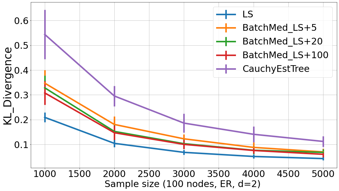
Next, we experiment the trade off between the batch-size (eg. batch size = [5, 20, 100]¹⁵¹⁵15We use batch size up to 100 to ensure there are enough batch size from simulation data, so that either mean and median can converge.) and the KL-divergence of our BatchAvgLeastSquares and BatchMedLeastSquares estimators in detail. As shown in Fig. 10 and Fig. 11, when batch size increases, the results are closer to the LeastSquares estimator. In other words, LeastSquares can be seen as a special case of either BatchAvgLeastSquares or BatchMedLeastSquares with one batch only. Thus, when batch size increases, the performances of BatchAvgLeastSquares and BatchMedLeastSquares are closer to the LeastSquares estimator. On the contrary, the CauchyEstTree estimator can be seen as the estimator with a batch size of $p$ . Therefore, with smaller batch size (eg. batch size $=p+5$ ), BatchAvgLeastSquares and BatchMedLeastSquares performs closer to the CauchyEstTree estimator.

Runtime comparison

We now give the amount of time spent by each algorithm to process a degree-5 ER graph on 100 nodes with 500 samples. LeastSquares algorithm takes 0.0096 seconds, BatchAvgLeastSquares with a batch size of $p+20$ takes 0.0415 seconds, BatchMedLeastSquares with a batch size of $p+20$ takes 0.0290 seconds, CauchyEstTree takes 0.6063 seconds, and CauchyEst takes 0.6307 seconds. The timings given above are representative of the relative running times of these algorithms across different graph sizes.

Takeaways

In summary, the LeastSquares estimator performs the best among all algorithms on uncontaminated datasets (both real and synthetic) generated from Gaussian Bayesian networks. This holds even when the data is ill-conditioned. However, if a fraction of the samples are contaminated, CauchyEst, CauchyEstTree and BatchMedLeastSquares outperform LeastSquares and BatchAvgLeastSquares by a large margin under different noise and graph types. If the data is not generated according to the input graph (i.e., the non-realizable/agnostic learning setting), then BatchAvgLeastSquares, CauchyEst, and CauchyEstTree have a better tradeoff between the error and sample complexity than the other algorithms, although we do not have a formal explanation.

Acknowledgements

This research/project is supported by the National Research Foundation, Singapore under its AI Singapore Programme (AISG Award No: AISG-PhD/2021-08-013).

References

[ABDH⁺20] Hassan Ashtiani, Shai Ben-David, Nicholas JA Harvey, Christopher Liaw, Abbas Mehrabian, and Yaniv Plan. Near-optimal sample complexity bounds for robust learning of gaussian mixtures via compression schemes. Journal of the ACM (JACM), 67(6):1–42, 2020.
[AGZ19] Bryon Aragam, Jiaying Gu, and Qing Zhou. Learning large-scale bayesian networks with the sparsebn package. Journal of Statistical Software, 91(1):1–38, 2019.
[AZ15] Bryon Aragam and Qing Zhou. Concave penalized estimation of sparse gaussian bayesian networks. The Journal of Machine Learning Research, 16(1):2273–2328, 2015.
[BCD20] Johannes Brustle, Yang Cai, and Constantinos Daskalakis. Multi-item mechanisms without item-independence: Learnability via robustness. In Proceedings of the 21st ACM Conference on Economics and Computation, pages 715–761, 2020.
[BGMV20] Arnab Bhattacharyya, Sutanu Gayen, Kuldeep S Meel, and NV Vinodchandran. Efficient distance approximation for structured high-dimensional distributions via learning. Advances in Neural Information Processing Systems, 33, 2020.
[BGPV20] Arnab Bhattacharyya, Sutanu Gayen, Eric Price, and NV Vinodchandran. Near-optimal learning of tree-structured distributions by chow-liu. arXiv preprint arXiv:2011.04144, 2020. ACM STOC 2021.
[BVH⁺16] Afonso S Bandeira, Ramon Van Handel, et al. Sharp nonasymptotic bounds on the norm of random matrices with independent entries. Annals of Probability, 44(4):2479–2506, 2016.
[CDKS20] C. L. Canonne, I. Diakonikolas, D. M. Kane, and A. Stewart. Testing bayesian networks. IEEE Transactions on Information Theory, 66(5):3132–3170, 2020.
[CDW19] Wenyu Chen, Mathias Drton, and Y Samuel Wang. On causal discovery with an equal-variance assumption. Biometrika, 106(4):973–980, 2019.
[CLL11] Tony Cai, Weidong Liu, and Xi Luo. A constrained l1 minimization approach to sparse precision matrix estimation. Journal of the American Statistical Association, 106(494):594–607, 2011.
[Das97] Sanjoy Dasgupta. The sample complexity of learning fixed-structure bayesian networks. Mach. Learn., 29(2-3):165–180, 1997.
[Dia16] Ilias Diakonikolas. Learning structured distributions. Handbook of Big Data, 267, 2016.
[DMR18] Luc Devroye, Abbas Mehrabian, and Tommy Reddad. The total variation distance between high-dimensional gaussians. arXiv preprint arXiv:1810.08693, 2018.
[Duc07] John Duchi. Derivations for linear algebra and optimization. Berkeley, California, 3(1):2325–5870, 2007.
[FHT08] Jerome Friedman, Trevor Hastie, and Robert Tibshirani. Sparse inverse covariance estimation with the graphical lasso. Biostatistics, 9(3):432–441, 2008.
[GDA20] Ming Gao, Yi Ding, and Bryon Aragam. A polynomial-time algorithm for learning nonparametric causal graphs. Advances in Neural Information Processing Systems, 33, 2020.
[GH17] Asish Ghoshal and Jean Honorio. Learning identifiable Gaussian bayesian networks in polynomial time and sample complexity. In Proceedings of the 31st International Conference on Neural Information Processing Systems, pages 6460–6469, 2017.
[Gut09] Allan Gut. An Intermediate Course in Probability. Springer New York, 2009.
[GZ20] Jiaying Gu and Qing Zhou. Learning big gaussian bayesian networks: Partition, estimation and fusion. Journal of Machine Learning Research, 21(158):1–31, 2020.
[Hau18] David Haussler. Decision theoretic generalizations of the PAC model for neural net and other learning applications. CRC Press, 2018.
[HSSC08] Aric Hagberg, Pieter Swart, and Daniel S Chult. Exploring network structure, dynamics, and function using networkx. Technical report, Los Alamos National Lab.(LANL), Los Alamos, NM (United States), 2008.
[HTW19] Trevor Hastie, Robert Tibshirani, and Martin Wainwright. Statistical learning with sparsity: the lasso and generalizations. Chapman and Hall/CRC, 2019.
[Hub04] Peter J Huber. Robust statistics, volume 523. John Wiley & Sons, 2004.
[JNG⁺19] Chi Jin, Praneeth Netrapalli, Rong Ge, Sham M Kakade, and Michael I Jordan. A short note on concentration inequalities for random vectors with subgaussian norm. arXiv preprint arXiv:1902.03736, 2019.
[KMR⁺94] Michael Kearns, Yishay Mansour, Dana Ron, Ronitt Rubinfeld, Robert E Schapire, and Linda Sellie. On the learnability of discrete distributions. In Proceedings of the twenty-sixth annual ACM symposium on Theory of computing, pages 273–282, 1994.
[KP83] H Kim and J Perl. ’a computational model for combined causal and diagnostic reasoning in inference systems’, 8th ijcai, 1983.
[Mue99] Ralph O Mueller. Basic principles of structural equation modeling: An introduction to LISREL and EQS. Springer Science & Business Media, 1999.
[Mul09] Stanley A Mulaik. Linear causal modeling with structural equations. CRC press, 2009.
[ORS07] Rainer Opgen-Rhein and Korbinian Strimmer. From correlation to causation networks: a simple approximate learning algorithm and its application to high-dimensional plant gene expression data. BMC systems biology, 1(1):1–10, 2007.
[Par20] Gunwoong Park. Identifiability of additive noise models using conditional variances. Journal of Machine Learning Research, 21(75):1–34, 2020.
[PB14] Jonas Peters and Peter Bühlmann. Identifiability of Gaussian structural equation models with equal error variances. Biometrika, 101(1):219–228, 2014.
[Pea86] Judea Pearl. Fusion, propagation, and structuring in belief networks. Artificial intelligence, 29(3):241–288, 1986.
[Pea88] Judea Pearl. Probabilistic reasoning in intelligent systems: networks of plausible inference. Morgan Kaufmann Publishers, San Francisco, Calif, 2nd edition edition, 1988.
[PK20] Gunwoong Park and Youngwhan Kim. Identifiability of Gaussian linear structural equation models with homogeneous and heterogeneous error variances. Journal of the Korean Statistical Society, 49(1):276–292, 2020.
[RV09] Mark Rudelson and Roman Vershynin. Smallest singular value of a random rectangular matrix. Communications on Pure and Applied Mathematics: A Journal Issued by the Courant Institute of Mathematical Sciences, 62(12):1707–1739, 2009.
[Scu09] Marco Scutari. Learning bayesian networks with the bnlearn r package. arXiv preprint arXiv:0908.3817, 2009.
[Scu20] Marco Scutari. bnlearn, 2020. Version 4.6.1.
[SHBM14] Marco Scutari, Phil Howell, David J Balding, and Ian Mackay. Multiple quantitative trait analysis using bayesian networks. Genetics, 198(1):129–137, 2014.
[SS05] Juliane Schafer and Korbinian Strimmer. A shrinkage approach to large-scale covariance matrix estimation and implications for functional genomics. Statistical applications in genetics and molecular biology, 4(1), 2005.
[Tsy08] Alexandre B Tsybakov. Introduction to nonparametric estimation. Springer Science & Business Media, 2008.
[Val84] Leslie G Valiant. A theory of the learnable. Communications of the ACM, 27(11):1134–1142, 1984.
[Wai19] Martin J Wainwright. High-dimensional statistics: A non-asymptotic viewpoint, volume 48. Cambridge University Press, 2019.

Appendix A Details on decomposition of KL divergence

In this section, we provide the full derivation of Eq. 1.

	$\displaystyle\;\mathrm{d_{KL}}(\mathcal{P},\mathcal{Q})$
$\displaystyle=$	$\displaystyle\;\int_{x}\mathcal{P}(x)\log\left(\frac{\mathcal{P}(x)}{\mathcal{Q}(x)}\right)dx$
$\displaystyle=$	$\displaystyle\;\int_{x}\mathcal{P}(x)\log\left(\frac{\Pi_{i=1}^{n}\mathcal{P}(x_{i}\mid\pi_{i}(x))}{\Pi_{i=1}^{n}\mathcal{Q}(x_{i}\mid\pi_{i}(x))}\right)dx$	$(\star)$
$\displaystyle=$	$\displaystyle\;\sum_{i=1}^{n}\int_{x}\mathcal{P}(x)\log\left(\frac{\mathcal{P}(x_{i}\mid\pi_{i}(x))}{\mathcal{Q}(x_{i}\mid\pi_{i}(x))}\right)dx$
$\displaystyle=$	$\displaystyle\;\sum_{i=1}^{n}\int_{x_{i},\pi_{i}(x)}\mathcal{P}(x_{i},\pi_{i}(x))\log\left(\frac{\mathcal{P}(x_{i}\mid\pi_{i}(x))}{\mathcal{Q}(x_{i}\mid\pi_{i}(x))}\right)dx_{i}d\pi_{i}(x)$	Marginalization

where $(\star)$ is due to the Bayesian network decomposition of joint probabilities. Let us define

\mathrm{d_{CP}}(\alpha^{*}_{i},\widehat{\alpha}_{i})=\int_{x_{i},\pi_{i}(x)}\mathcal{P}(x_{i},\pi_{i}(x))\log\left(\frac{\mathcal{P}(x_{i}\mid\pi_{i}(x))}{\mathcal{Q}(x_{i}\mid\pi_{i}(x))}\right)dx_{i}d\pi_{i}(x)

where each $\widehat{\alpha}_{i}$ and $\alpha^{*}_{i}$ represent the parameters that relevant to variable $X_{i}$ from $\widehat{\alpha}$ and $\alpha^{*}$ respectively. Under this notation, we can write $\mathrm{d_{KL}}(\mathcal{P},\mathcal{Q})=\sum_{i=1}^{n}\mathrm{d_{CP}}(\alpha^{*}_{i},\widehat{\alpha}_{i})$ .

Fix a variable of interest $Y$ with parents $X_{1},\ldots,X_{p}$ , each with coefficient $c_{i}$ , and variance $\sigma^{2}$ . That is, $Y=\eta_{y}+\sum_{i=1}^{p}c_{i}X_{i}$ for some $\eta_{y}\sim N(0,\sigma^{2})$ that is independent of $X_{1},\ldots,X_{p}$ . By denoting $X=x$ (i.e. $X_{1}=x_{1},\ldots,X_{p}=x_{p}$ ) and $c=(c_{1},\ldots,c_{p})$ , we can write the conditional distribution density of $Y$ as

\Pr\left(y\mid x,c,\sigma\right)=\frac{1}{\sigma\sqrt{2\pi}}\exp\left(-\frac{1}{2\sigma^{2}}\cdot\left(y-\sum_{i=1}^{p}c_{i}X_{i}\right)^{2}\right)

We now analyze $\mathrm{d_{CP}}(\alpha^{*}_{y},\widehat{\alpha}_{y})$ with respect to the our estimates $\widehat{\alpha}_{y}=(\widehat{A},\widehat{\sigma}_{y})$ and the hidden true parameters $\alpha^{*}_{y}=(A,\sigma_{y})$ , where $\widehat{A}=(\widehat{a}_{y\leftarrow 1},\ldots,\widehat{a}_{y\leftarrow p})$ and $A=(a_{y\leftarrow 1},\ldots,a_{y\leftarrow p})$ .

With respect to variable $Y$ , we see that

		$\displaystyle\;\mathrm{d_{CP}}(\alpha^{*}_{y},\widehat{\alpha}_{y})$
	$\displaystyle=$	$\displaystyle\;\int_{x,y}\mathcal{P}(x,y)\ln\left(\frac{\frac{1}{\sigma_{y}\sqrt{2\pi}}\exp\left(-\frac{1}{2\sigma^{2}}\cdot\left(y-\sum_{i=1}^{p}a_{y\leftarrow i}X_{i}\right)^{2}\right)}{\frac{1}{\widehat{\sigma}_{y}\sqrt{2\pi}}\exp\left(-\frac{1}{2\widehat{\sigma}_{y}^{2}}\cdot\left(y-\sum_{i=1}^{p}\widehat{a}_{y\leftarrow i}X_{i}\right)^{2}\right)}\right)dy\ dx$
	$\displaystyle=$	$\displaystyle\;\ln\left(\frac{\widehat{\sigma}_{y}}{\sigma_{y}}\right)-\frac{1}{2\sigma_{y}^{2}}\cdot\mathbb{E}_{x,y}\left(y-\sum_{i=1}^{p}a_{y\leftarrow i}X_{i}\right)^{2}+\frac{1}{2\widehat{\sigma}_{y}^{2}}\cdot\mathbb{E}_{x,y}\left(y-\sum_{i=1}^{p}\widehat{a}_{y\leftarrow i}X_{i}\right)^{2}$
	$\displaystyle=$	$\displaystyle\;\ln\left(\frac{\widehat{\sigma}_{y}}{\sigma_{y}}\right)-\frac{1}{2\sigma_{y}^{2}}\cdot\mathbb{E}_{x,y}\left(y-A^{\top}X\right)^{2}+\frac{1}{2\widehat{\sigma}_{y}^{2}}\cdot\mathbb{E}_{x,y}\left(y-\widehat{A}^{\top}X\right)^{2}$

By defining $\Delta=\widehat{A}-A$ , we can see that for any instantiation of $y,X_{1},\ldots,X_{p}$ ,

	$\displaystyle\;\left(y-\widehat{A}^{\top}X\right)^{2}$
$\displaystyle=$	$\displaystyle\;\left(y-(\Delta+A)^{\top}X\right)^{2}$	By definition of $\Delta$
$\displaystyle=$	$\displaystyle\;\left((y-A^{\top}X)-\Delta^{\top}X\right)^{2}$
$\displaystyle=$	$\displaystyle\;(y-A^{\top}X)^{2}-2(y-A^{\top}X)(\Delta^{\top}X)+\left(\Delta^{\top}X\right)^{2}$
$\displaystyle=$	$\displaystyle\;(y-A^{\top}X)^{2}-2\left(y\Delta^{\top}X-A^{\top}X\Delta^{\top}X\right)+\left(\Delta^{\top}X\right)^{2}$
$\displaystyle=$	$\displaystyle\;(y-A^{\top}X)^{2}-2\left(yX^{\top}\Delta-A^{\top}XX^{\top}\Delta\right)+\Delta^{\top}XX^{\top}\Delta$	Since $\Delta^{\top}X$ is just a number

Denote the covariance matrix with respect to $X_{1},\ldots,X_{p}$ as $M\in\mathbb{R}^{p\times p}$ , where $M_{i,j}=\mathbb{E}\left[X_{i}X_{j}\right]$ . Then, we can further simplify $\mathrm{d_{CP}}(\alpha^{*}_{y},\widehat{\alpha}_{y})$ as follows:

	$\displaystyle\;\mathrm{d_{CP}}(\alpha^{*}_{y},\widehat{\alpha}_{y})$
$\displaystyle=$	$\displaystyle\;\ln\left(\frac{\widehat{\sigma}_{y}}{\sigma_{y}}\right)-\frac{1}{2\sigma_{y}^{2}}\cdot\mathbb{E}_{x,y}\left(y-A^{\top}X\right)^{2}+\frac{1}{2\widehat{\sigma}_{y}^{2}}\cdot\mathbb{E}_{x,y}\left(y-\widehat{A}^{\top}X\right)^{2}$	From above
$\displaystyle=$	$\displaystyle\;\ln\left(\frac{\widehat{\sigma}_{y}}{\sigma_{y}}\right)-\frac{1}{2\sigma_{y}^{2}}\cdot\mathbb{E}_{x,y}\left(y-A^{\top}X\right)^{2}$
	$\displaystyle\;+\frac{1}{2\widehat{\sigma}_{y}^{2}}\cdot\mathbb{E}_{x,y}\left[(y-A^{\top}X)^{2}-2\left(yX^{\top}\Delta-A^{\top}XX^{\top}\Delta\right)+\Delta^{\top}XX^{\top}\Delta\right]$	From above
$\displaystyle=$	$\displaystyle\;\ln\left(\frac{\widehat{\sigma}_{y}}{\sigma_{y}}\right)-\frac{1}{2\sigma_{y}^{2}}\cdot\mathbb{E}_{x,y}\eta_{y}^{2}+\frac{1}{2\widehat{\sigma}_{y}^{2}}\cdot\mathbb{E}_{x,y}\left[\eta_{y}^{2}-2\left(\eta_{y}X^{\top}\Delta\right)+\Delta^{\top}XX^{\top}\Delta\right]$	$({\dagger})$
$\displaystyle=$	$\displaystyle\;\ln\left(\frac{\widehat{\sigma}_{y}}{\sigma_{y}}\right)-\frac{1}{2\sigma_{y}^{2}}\cdot\sigma_{y}^{2}+\frac{1}{2\widehat{\sigma}_{y}^{2}}\cdot\left[\sigma_{y}^{2}-0+\Delta^{\top}M\Delta\right]$	$(\ast)$
$\displaystyle=$	$\displaystyle\;\ln\left(\frac{\widehat{\sigma}_{y}}{\sigma_{y}}\right)-\frac{1}{2}+\frac{\sigma_{y}^{2}}{2\widehat{\sigma}_{y}^{2}}+\frac{\Delta^{\top}M\Delta}{2\widehat{\sigma}_{y}^{2}}$
$\displaystyle=$	$\displaystyle\;\ln\left(\frac{\widehat{\sigma}_{y}}{\sigma_{y}}\right)+\frac{\sigma_{y}^{2}-\widehat{\sigma}_{y}^{2}}{2\widehat{\sigma}_{y}^{2}}+\frac{\Delta^{\top}M\Delta}{2\widehat{\sigma}_{y}^{2}}$

where $({\dagger})$ is because $y=\eta_{y}+A^{\top}X$ while $(\ast)$ is because $\eta_{y}\sim N(0,\sigma_{y}^{2})$ , $\mathbb{E}_{x,y}\left(\eta_{y}X^{\top}\Delta\right)=\mathbb{E}_{x,y}\eta_{y}\cdot\mathbb{E}_{x,y}X^{\top}\Delta=0$ , and $\mathbb{E}_{x,y}\Delta^{\top}XX^{\top}\Delta=\Delta^{\top}(\mathbb{E}_{x,y}XX^{\top})\Delta=\Delta^{\top}M\Delta$ .

In conclusion, we have

\mathrm{d_{KL}}(\mathcal{P},\mathcal{Q})=\sum_{i=1}^{n}\mathrm{d_{CP}}(\alpha^{*}_{i},\widehat{\alpha}_{i})=\sum_{i=1}^{n}\ln\left(\frac{\widehat{\sigma}_{i}}{\sigma_{i}}\right)+\frac{\sigma_{i}^{2}-\widehat{\sigma}_{i}^{2}}{2\widehat{\sigma}_{i}^{2}}+\frac{\Delta_{i}^{\top}M_{i}\Delta_{i}}{2\widehat{\sigma}_{i}^{2}}

(3)

Appendix B Deferred proofs

This section provides the formal proofs that were deferred in favor for readability. For convenience, we will restate the statements before proving them.

The next two lemmata Lemma 2.6 and Lemma 2.7 are used in the proof of Lemma 3.2, which is in turn used in the proof of Theorem 3.1. We also use Lemma 2.6 in the proof of Lemma 3.5. The proof of Lemma 2.6 uses the standard result of Lemma B.1.

Lemma B.1 ([RV09]; Theorem 6.1 and Equation 6.10 in [Wai19]).

Let $\ell\geq d$ and $G\in\mathbb{R}^{\ell\times d}$ be a matrix with i.i.d. $N(0,1)$ entries. Denote $\sigma_{\min}(G)$ as the smallest singular value of $G$ . Then, for any $0<t<1$ , we have $\Pr\left(\sigma_{\min}(G)\geq\sqrt{\ell}(1-t)-\sqrt{d}\right)\leq\exp\left(-\ell t^{2}/2\right)$ .

See 2.6

Proof of Lemma 2.6.

Observe that $G^{\top}G$ is symmetric, thus $(G^{\top}G)^{-1}$ is also symmetric and the eigenvalues of $G^{\top}G$ equal the singular values of $G^{\top}G$ . Also, note that event that $G^{\top}G$ is singular has measure 0.¹⁶¹⁶16Consider fixing all but one arbitrary entry of $G$ . The event of this independent $N(0,1)$ entry making $\det(G^{\top}G)=0$ has measure 0.

By definition of operation norm, $\left\lVert(G^{\top}G)^{-1}\right\rVert$ equals the square root of maximum eigenvalue of

((G^{\top}G)^{-1})^{\top}((G^{\top}G)^{-1})=((G^{\top}G)^{-1})^{2},

where the equality is because $(G^{\top}G)^{-1}$ is symmetric. Since $G^{\top}G$ is invertible, we have $\|(G^{\top}G)^{-1}\|=1/\|G^{\top}G\|$ , which is equal to the inverse of minimum eigenvalue $\lambda_{\min}(G^{\top}G)$ of $G^{\top}G$ , which is in turn equal to the square of minimum singular value $\sigma_{\min}(G)$ of $G$ .

Therefore, the following holds with probability at least $1-\exp\left(-kc_{1}^{2}/2\right)$ :

\left\lVert\left(G^{\top}G\right)^{-1}\right\rVert=\frac{1}{\left\lVert G^{\top}G\right\rVert}=\frac{1}{\lambda_{\min}(G^{\top}G)}=\frac{1}{\sigma_{\min}^{2}(G)}\leq\frac{1}{\left(\sqrt{k}(1-c_{1})-\sqrt{d}\right)^{2}}\leq\frac{1}{\left(1-2c_{1}\right)^{2}k}

where the second last inequality is due to Lemma B.1 and the last inequality holds when $k\geq d/c_{1}^{2}$ . ∎

See 2.7

Proof of Lemma 2.7.

Let us denote $g_{r}\in\mathbb{R}^{k}$ as the $r^{th}$ row of $G^{\top}$ . Then, we see that $\|G^{\top}\eta\|_{2}^{2}=\sum_{r=1}^{p}\langle g_{r},\eta\rangle^{2}$ . For any row $r$ , we see that $\langle g_{r},\eta\rangle=\|\eta\|_{2}\cdot\langle g_{r},\eta/\|\eta\|_{2}\rangle$ . We will bound values of $\|\eta\|_{2}$ and $|\langle g_{r},\eta/\|\eta\|_{2}\rangle|$ separately.

It is well-known (e.g. see [JNG⁺19, Lemma 2]) that the norm of a Gaussian vector concentrates around its mean. So, $\Pr\left(\|\eta\|_{2}\leq 2\sigma\sqrt{k}\right)\leq 2\exp\left(-2k\right)$ . Since $g_{r}\sim N(0,I_{k})$ and $\eta$ are independent, we see that $\langle g_{r},\eta/\|\eta\|_{2}\rangle\sim N(0,1)$ . By standard Gaussian bounds, we have that $\Pr\left[|\langle g_{r},\eta/\|\eta\|_{2}\rangle|\geq c_{2}\right]\leq\exp\left(-c_{2}^{2}/2\right)$ .

By applying a union bound over these two events, we see that $\|\langle g_{r},\eta\rangle\|<2\sigma c_{2}\sqrt{k}$ for any row with probability $2\exp\left(-2k\right)+\exp\left(-c_{2}^{2}/2\right)$ . The claim follows from applying a union bound over all $p$ rows. ∎

See 2.8

Proof of Lemma 2.8.

Let $S_{>\tau}=\sum_{i=1}^{m}\mathbbm{1}_{X_{i}>\tau}$ be the number of values that are larger than $\tau$ , where $\mathbb{E}[\mathbbm{1}_{X_{i}>\tau}]=\Pr(X\geq\tau)$ . Similarly, let $S_{<-\tau}$ be the number of values that are smaller than $-\tau$ . If $S_{>\tau}<m/2$ and $S_{<-\tau}<m/2$ , then we see that $\mathrm{median}\left\{X_{1},\ldots,X_{m}\right\}\in[-\tau,\tau]$ .

For a random variable $X\sim\mathrm{Cauchy}(0,1)$ , we know that $\Pr(X\leq x)=1/2+\arctan(x)/\pi$ . For $0<\tau<1$ , we see that $\Pr(X\geq\tau)=1/2-\arctan(\tau)/\pi\leq 1/2-\tau/4$ . By additive Chernoff bounds, we see that

\Pr\left(S_{>\tau}\geq\frac{m}{2}\right)\leq\exp\left(-\frac{2m^{2}\tau^{2}}{16m}\right)=\exp\left(-\frac{m\tau^{2}}{8}\right)

Similarly, we have $\Pr\left(S_{<-\tau}\geq m/2\right)\leq\exp\left(-m\tau^{2}/8\right)$ . The claim follows from a union bound over the events $S_{>\tau}\geq m/2$ and $S_{<-\tau}\geq m/2$ . ∎

Appendix C Median absolute deviation

In this section, we give a pseudo-code of the well-known Median Absolute Deviation (MAD) estimator (see [Hub04] for example) which we use for the component-wise variance recovery in the contaminated setting. The scale factor, $1/\Phi^{-1}(3/4)\approx 1.4826$ below, is needed to make the estimator unbiased.

Algorithm 8 MAD: Variance recovery in the contaminated setting

1:Input: Contaminated samples

\{x_{1},x_{2},\dots,x_{m}\}

from a univariate Gausssian

\widehat{\mu}\leftarrow\mathrm{median}\left\{x_{1},x_{2},\dots,x_{m}\right\}

\widehat{\sigma}\leftarrow 1.4826\cdot\mathrm{median}\left\{|x_{1}-\widehat{\mu}|,|x_{2}-\widehat{\mu}|,\dots,|x_{m}-\widehat{\mu}|\right\}

4:return

\widehat{\sigma}

Learning Sparse Fixed-Structure Gaussian Bayesian Networks

Abstract

1 Introduction

Assumption 1.1.

1.1 Our contributions

1.2 Outline of paper

1.3 Further related work

2 Preliminaries

2.1 Notation

2.2 Basic facts and results

Fact 2.1.

Fact 2.2.

Fact 2.3 (Theorem 2.2 in [Gut09])).

Lemma 2.4 (Equation 2.19 in [Wai19]).

Lemma 2.5 (Consequence of Corollary 3.11 in [BVH+16]).

Lemma 2.6.

Proof.

Lemma 2.7.

Proof.

Lemma 2.8.

Proof.

2.3 Distance and divergence between probability distributions

Definition 2.9 (Total variational (TV) distance).

Definition 2.10 (Kullback–Leibler (KL) divergence).

Fact 2.11 (Pinsker’s inequality).

2.4 Decomposing the KL divergence

2.5 Bounding dCP\mathrm{d_{CP}} for an arbitrary variable

Proposition 2.12 (Implication of KL decomposition).

Proof.

2.6 Two-phased recovery approach

Lemma 2.13.

Proof.

Corollary 2.14 (Guarantees of VarianceRecovery).

Proof.

3 Coefficient estimators based on linear least squares

3.1 Vanilla least squares

Theorem 3.1 (Distribution learning using LeastSquares).

Lemma 3.2.

Proof.

Lemma 3.3.

Proof.

Proof of Theorem 3.1.

3.2 Interpolating between batch size and number of batches

Theorem 3.4 (Distribution learning using BatchAvgLeastSquares).

Lemma 3.5.

Proof.

Lemma 3.6 (Coefficient recovery guarantees of BatchAvgLeastSquares).

Proof.

Proof of Theorem 3.4.

4 Coefficient recovery algorithm based on Cauchy random variables

Lemma 4.1.

Proof.

Lemma 4.2.

Proof.

4.1 Special case of polytree Bayesian networks

Corollary 4.3.

Proof.

Theorem 4.4 (Distribution learning using CauchyEstTree).

Lemma 4.5.

Proof.

Lemma 4.6.

Proof.

Proof of Theorem 4.4.

5 Hardness for learning Gaussian Bayesian networks

Fact 5.1 ([DMR18]).

Theorem 5.2.

Proof.

Theorem 5.3.

Claim 5.4.

Proof.

Claim 5.5.

Proof.

Proof of Theorem 5.3.

6 Experiments

General Setup

Algorithms

Synthetic data

Real-world datasets

Contaminated synthetic data

Contaminated real-world datasets

Lemma 2.5 (Consequence of Corollary 3.11 in [BVH⁺16]).

2.5 Bounding $\mathrm{d_{CP}}$ for an arbitrary variable