Learning Representation from Neural Fisher Kernel with Low-rank Approximation

Ruixiang Zhang
Mila, Université de Montréal
[email protected]
&Shuangfei Zhai, Etai Littwin, Josh Susskind
Apple Inc.
{szhai,elittwin,jsusskind}@apple.com

Abstract

In this paper, we study the representation of neural networks from the view of kernels. We first define the Neural Fisher Kernel (NFK), which is the Fisher Kernel (Jaakkola and Haussler, 1998) applied to neural networks. We show that NFK can be computed for both supervised and unsupervised learning models, which can serve as a unified tool for representation extraction. Furthermore, we show that practical NFKs exhibit low-rank structures. We then propose an efficient algorithm that computes a low rank approximation of NFK, which scales to large datasets and networks. We show that the low-rank approximation of NFKs derived from unsupervised generative models and supervised learning models gives rise to high-quality compact representations of data, achieving competitive results on a variety of machine learning tasks.

1 Introduction

Modern deep learning systems rely on finding good representations of data. For supervised learning models with feed forward neural networks, representations can naturally be equated with the activations of each layer. Empirically, the community has developed a set of effective heuristics for representation extraction given a trained network. For example, ResNets (He et al., 2016) trained on Imagenet classification yield intermediate layer representations that can benefit downstream tasks such as object detection and semantic segmentation. The logits layer of a trained neural network also captures rich correlations across classes which can be distilled to a weaker model (Knowledge Distillation) (Hinton et al., 2015).

Despite empirical prevalence of using intermediate layer activations as data representation, it is far from being the optimal approach to representation extraction. For supervised learning models, it remains a manual procedure that relies on trial and error to select the optimal layer from a pre-trained model to facilitate transfer learning. Similar observations also apply to unsupervised learning models including GANs (Goodfellow et al., 2014), VAEs (Kingma and Welling, 2014), as evident from recent studies (Chen et al., 2020a) that the quality of representation in generative models heavily depends on the choice of layer from which we extract activations as features. Furthermore, although that GANs and VAEs are known to be able to generate high-quality samples from the data distribution, there is no strong evidence that they encode explicit layerwise representations to similar quality as in supervised learning models, which implies that there does not exist a natural way to explicitly extract a representation from intermediate layer activations in unsupervisedly pre-trained generative models. Additionally, layer activations alone do not suffice to reach the full power of learned representations hidden in neural network models, as shown in recent works (Mu et al., 2020) that incorporating additional gradients-based features into representation leads to substantial improvement over solely using activations-based features.

In light of these constraints, we are interested in the question: is there a principled method for representation extraction beyond layer activations? In this work, we turn to the kernel view of neural networks. Recently, initiated by the Neural Tangent Kernel (NTK) (Jacot et al., 2018) work, there have been growing interests in the kernel interpretation of neural networks. It was shown that neural networks in the infinite width regime are reduced to kernel regression with the induced NTK. Our key intuition is that, the kernel machine induced by the neural network provides a powerful and principled way of investigating the non-linear feature transformation in neural networks using the linear feature space of the kernel. Kernel machines provide drastically different representations than layer activations, where the knowledge of a neural network is instantiated by the induced kernel function over data points.

In this work, we propose to make use of the linear feature space of the kernel, associated with the pre-trained neural network model, as the data representation of interest. To this end, we made novel contributions on both theoretical and empirical side, as summarized below.

•

We propose Neural Fisher Kernel (NFK) as a unified and principled kernel formulation for neural networks models in both supervised learning and unsupervised learning settings.
•

We introduce a highly efficient and scalable algorithm for low-rank kernel approximation of NFK, which allows us to obtain a compact yet informative feature embedding as the data representation.
•

We validate the effectiveness of proposed approach from NFK in unsupervised learning, semi-supervised learning and supervised learning settings, showing that our method enjoys superior sample efficiency and representation quality.

2 Preliminary and Related Works

In this section, we present technical background and formalize the motivation. We start by introducing the notion of data representation from the perspective of kernel methods, then introduce the connections between neural network models and kernel methods.

Notations. Throughout this paper, we consider dataset with $N$ data examples ${\mathcal{D}}\equiv\left\{\left({\mathbf{x}}_{i},y_{i}\right)\right\}$ , we use $p({\mathbf{x}})$ to denote the probability density function for the data distribution and use $p_{\mathrm{data}}({\mathbf{x}})$ to denote the empirical data distribution from ${\mathcal{D}}$ .

Kernel Methods. Kernel methods (Hofmann et al., 2008) have long been a staple of practical machine learning. At their core, a kernel method relies on a kernel function which acts as a similarity function between different data examples in some feature space. Here we consider positive definite kernels $\mathcal{K}:\mathcal{X}\times\mathcal{X}\rightarrow\mathbb{R}$ over a metric space $\mathcal{X}$ which defines a reproducing kernel Hilbert space ${\mathcal{H}}$ of function from $\mathcal{X}$ to $\mathbb{R}$ , along with a mapping function $\varphi:\mathcal{X}\rightarrow{\mathcal{H}}$ , such that the kernel function can be decomposed into the inner product $\mathcal{K}({\mathbf{x}},{\mathbf{z}})=\langle\varphi({\mathbf{x}}),\varphi({\mathbf{z}})\rangle$ . Kernel methods aim to find a predictive linear function $f({\mathbf{x}})=\langle f,\varphi({\mathbf{x}})\rangle_{{\mathcal{H}}}$ in ${\mathcal{H}}$ , which gives label output prediction for each data point ${\mathbf{x}}\in\mathcal{X}$ . The kernel maps each data example ${\mathbf{x}}\in\mathcal{X}$ to a linear feature space $\varphi({\mathbf{x}})$ , which is the data representation of interest. Given dataset ${\mathcal{D}}$ , the predictive model function $f$ is typically estimated via Kernel Ridge Regression (KRR), $\widehat{f}={\operatorname{argmin}}_{f\in\mathcal{H}}\frac{1}{N}\sum_{i=1}^{N}\left(f\left({\mathbf{x}}_{i}\right)-y_{i}\right)^{2}+\lambda\|f\|_{\mathcal{H}}^{2}$ .

Neural Networks and Kernel Methods. A long line of works (Neal, 1996, Williams, 1996, Roux and Bengio, 2007, Hazan and Jaakkola, 2015, Lee et al., 2018, de G. Matthews et al., 2018, Jacot et al., 2018, Chen and Xu, 2021, Geifman et al., 2020, Belkin et al., 2018, Ghorbani et al., 2020), have studied that many kernel formulations can be associated to neural networks, while most of them correspond to neural network where being fixed kernels (e.g. Laplace kernel, Gaussian kernel) or only the last layer is trained, e.g., Conjugate Kernel (CK) (Daniely et al., 2016), also called as NNGP kernel (Lee et al., 2018). On the other hand, Neural Tangent Kernel (NTK) (Jacot et al., 2018) is a fundamentally different formulation corresponding to training the entire infinitely wide neural network models. Let $f({\bm{\theta}};{\mathbf{x}})$ denote a neural network function with parameters ${\bm{\theta}}$ , then the empirical NTK is defined as $\mathcal{K}_{\mathrm{ntk}}({\mathbf{x}},{\mathbf{z}})=\left\langle\nabla_{{\bm{\theta}}}f({\bm{\theta}};{\mathbf{x}}),\nabla_{{\bm{\theta}}}f({\bm{\theta}};{\mathbf{z}})\right\rangle$ . (Jacot et al., 2018, Lee et al., 2018) showed that under the so-called NTK parametrization and other proper assumptios, the function $f({\mathbf{x}};{\bm{\theta}})$ learned by training the neural network model with gradient descent is equivalent to the function estimated via ridgeless KRR using $\mathcal{K}_{\mathrm{ntk}}$ as the kernel. For finite-width neural networks, by taking first-order Taylor expansion of funnction $f$ around the ${\bm{\theta}}$ , kernel regression under $\mathcal{K}_{\mathrm{ntk}}$ can be seen as linearized neural network model at parameter ${\bm{\theta}}$ , suggesting that pre-trained neural network models can also be studied and approximated from the perspective of kernel methods.

Fisher Kernel. The Fisher Kernel (FK) is first introduced in the seminal work (Jaakkola and Haussler, 1998). Given a probabilistic generative model $p_{{\bm{\theta}}}(x)$ , the Fisher kernel is defined as: $\mathcal{K}_{\mathrm{fisher}}({\mathbf{x}},{\mathbf{z}})=\nabla_{{\bm{\theta}}}\log p_{{\bm{\theta}}}({\mathbf{x}})^{\top}\mathcal{I}^{-1}\nabla_{{\bm{\theta}}}\log p_{{\bm{\theta}}}({\mathbf{z}})=U_{{\mathbf{x}}}^{\top}{\mathcal{I}}^{-1}U_{{\mathbf{z}}}$ where $U_{{\mathbf{x}}}=\nabla_{{\bm{\theta}}}\log p_{{\bm{\theta}}}({\mathbf{x}})$ is the so-called Fisher score and $\mathcal{I}$ is the Fisher Information Matrix (FIM) defined as the covariance of the Fisher score: ${\mathcal{I}}=\mathbb{E}_{{\mathbf{x}}\sim p_{{\bm{\theta}}}({\mathbf{x}})}\nabla_{{\bm{\theta}}}\log p_{{\bm{\theta}}}({\mathbf{x}})\nabla_{{\bm{\theta}}}\log p_{{\bm{\theta}}}({\mathbf{x}})^{\top}$ . Then the Fisher vector is defined as $V_{{\mathbf{x}}}={\mathcal{I}}^{-\frac{1}{2}}\nabla_{{\bm{\theta}}}\log p_{{\bm{\theta}}}({\mathbf{x}})={\mathcal{I}}^{-\frac{1}{2}}U_{{\mathbf{x}}}$ . One can utilize the Fisher Score as a mapping from the data space $\mathcal{X}$ to parameter space $\Theta$ , and obtain representations that are linearized. As proposed in (Jaakkola and Haussler, 1998, Perronnin and Dance, 2007), the Fisher vector $V_{{\mathbf{x}}}$ can be used as the feature representation derived from probabilistic generative models, which was shown to be superior to hand-crafted visual descriptors in a variety of computer vision tasks.

Generative Models In this work, we consider a variety of representative deep generative models, including generative adversarial networks (GANs) (Goodfellow et al., 2014), variational auto-encoders (VAEs) (Kingma and Welling, 2014), as well we normalizing flow models (Dinh et al., 2015) and auto-regressive models (van den Oord et al., 2016). Please refer to (Salakhutdinov, 2014) for more technical details on generative models.

Refer to caption — Figure 1: Overview of our proposed approach. Given a pre-trained neural network model, which can be either an unsupervised generative model $p_{{\bm{\theta}}}({\mathbf{x}})$ (e.g. GANs, VAEs), or a supervised learning model $p_{{\bm{\theta}}}({\mathbf{y}}|{\mathbf{x}})$ , we aim to extract a compact yet informative representation from it. By reinterpreting various families of models as energy-based models (EBM), we introduce Neural Fisher Kernel (NFK) ${\mathcal{K}}_{\text{nfk}}$ as a principled and unified kernel formulation for neural network models (Section. 3.1). We introduce a highly efficient and scalable kernel approximation algorithm (Section. 3.2) to obtain the low-dimensional feature embedding ${\mathbf{e}}_{{\mathbf{x}}}$ , which serves as the extracted data representation from NFK.

3 Learning Representation from Neural Fisher Kernel

We aim to propose a general and efficient method for extracting high-quality representation from pre-trained neural network models. As formalized in previous section, we can describe the outline of our proposed approach as: given a pre-trained neural network model $f({\mathbf{x}};{\bm{\theta}})$ (either unsupervised generative model $p({\mathbf{x}};{\bm{\theta}})$ or supervised learning model $p({\mathbf{y}}\mid{\mathbf{x}};{\bm{\theta}})$ ), with pre-trained weights ${\bm{\theta}}$ , we adopt the kernel formulation $\mathcal{K}_{f}$ induced by model $f({\mathbf{x}};{\bm{\theta}})$ and make use of the associated linear feature embedding $\varphi({\mathbf{x}})$ of the kernel $\mathcal{K}_{f}$ as the feature representation of data ${\mathbf{x}}$ . We present an overview introduction to illustrate our approach in Figure. 1.

At this point, however, there exist both theoretical difficulties and practical challenges which impede a straightforward application of our proposed approach. On the theoretical side, the NTK theory is only developed in supervised learning setting, and its extension to unsupervised learning is not established yet. Though Fisher kernel is immediately applicable in unsupervised learning setting, deriving Fisher vector from supervised learning model $p({\mathbf{y}}\mid{\mathbf{x}};{\bm{\theta}})$ can be tricky, which needs the log-density estimation of marginal distribution $p_{{\bm{\theta}}}({\mathbf{x}})$ from $p({\mathbf{y}}\mid{\mathbf{x}};{\bm{\theta}})$ . Note that it is a drastically different problem from previous works (Achille et al., 2019) where Fisher kernel is applied to the joint distribution over $p({\mathbf{x}},{\mathbf{y}})$ . On the practical efficiency side, the dimensionality of the feature space associated with NTK or FK is same as the number of model parameters $|{\bm{\theta}}|$ , which poses unmanageably high time and space complexity when it comes to modern large-scale neural network models. Additionally, the size of the NTK scales quadratically with the number of classes in multi-class supervised learning setting, which gives rise to more efficiency concerns.

To address the kernel formulation issue, we propose Neural Fisher Kernel (NFK) in Sec. 3.1 as a unified kernel for both supervised and unsupervised learning models. To tackle the efficiency challenge, we investigate the structural properties of the proposed NFK and propose a highly scalable low-rank kernel approximation algorithm in Sec. 3.2 to extract compact low-dimensional feature representation from NFK.

3.1 Neural Fisher Kernel

In this section, we propose Neural Fisher Kernel (NFK) as a principled and general kernel formulation for neural network models. The key intuition is that we can extend classical Fisher kernel theory to unify the procedure of deriving Fisher vector from supervised learning models and unsupervised learning models by using Energy-based Model (EBM) formulation.

3.1.1 Unsupervised NFK

We consider unsupervised probabilistic generative models $p_{{\bm{\theta}}}({\mathbf{x}})=p({\mathbf{x}};{\bm{\theta}})$ here. Our proposed NFK formulation can be applied to all generative models with tractable evaluation (or approximation) of $\nabla_{{\bm{\theta}}}\log p_{{\bm{\theta}}}({\mathbf{x}})$ .

GANs. We consider the EBM formulation of GANs (Dai et al., 2017, Zhai et al., 2019, Che et al., 2020). Given pre-trained GAN model, we use $D({\mathbf{x}};{\bm{\theta}})$ to denote the output of the discriminator $D$ , and use $G({\mathbf{h}})$ to denote the output of generator $G$ given latent code ${\mathbf{h}}\sim p({\mathbf{h}})$ . As a brief recap, GANs can be interpreted as an implementation of EBM training with a variational distribution, where we have the energy-function $E({\mathbf{x}};{\bm{\theta}})=-D({\mathbf{x}};{\bm{\theta}})$ . Please refer to (Zhai et al., 2019, Che et al., 2020) for more details. Thus we have the unnormalized density function $p_{{\bm{\theta}}}({\mathbf{x}})\propto e^{-E({\mathbf{x}};{\bm{\theta}})}$ given by the GAN model. Following (Zhai et al., 2019), we can then derive the Fisher kernel $\mathcal{K}_{\mathrm{nfk}}$ and Fisher vector from standard GANs as shown below:

\begin{split}&\mathcal{K}_{\mathrm{nfk}}({\mathbf{x}},{\mathbf{z}})=\langle V_{{\mathbf{x}}},V_{{\mathbf{z}}}\rangle\quad\quad V_{{\mathbf{x}}}=(\texttt{diag}(\mathcal{I})^{-\frac{1}{2}})U_{{\mathbf{x}}}\\ &U_{{\mathbf{x}}}=\nabla_{{\bm{\theta}}}D({\mathbf{x}};{\bm{\theta}})-\mathbb{E}_{{\mathbf{h}}\sim p({\mathbf{h}})}\nabla_{{\bm{\theta}}}D(G({\mathbf{h}});{\bm{\theta}})\\ \end{split}

(1)

where ${\mathbf{x}},{\mathbf{z}}\in\mathcal{X}$ , $\mathcal{I}=\mathbb{E}_{{\mathbf{h}}\sim p({\mathbf{h}})}\left[U_{G({\mathbf{h}})}U_{G({\mathbf{h}})}^{\top}\right]$ . Note that we use diagonal approximation of FIM throughout this work for the consideration of scalability.

VAEs. Given a VAE model pre-trained via maximizing the variational lower-bound ELBO $\mathcal{L}_{\mathrm{ELBO}}(\mathbf{x})\equiv\mathbb{E}_{q(\mathbf{h}\mid\mathbf{x})}\left[\log\frac{p(\mathbf{x},\mathbf{h})}{q(\mathbf{h}\mid\mathbf{x})}\right]$ , we can approximate the marginal log-likelihood $\log p_{{\bm{\theta}}}({\bm{\theta}})$ by evaluating $\mathcal{L}_{\mathrm{ELBO}}(\mathbf{x})$ via Monte-Carlo estimations or importance sampling techniques (Burda et al., 2016). Thus we have our NFK formulation as

\begin{split}&\mathcal{K}_{\mathrm{nfk}}({\mathbf{x}},{\mathbf{z}})=\langle V_{{\mathbf{x}}},V_{{\mathbf{z}}}\rangle\quad\quad V_{{\mathbf{x}}}=(\texttt{diag}(\mathcal{I})^{-\frac{1}{2}})U_{{\mathbf{x}}}\\ &U_{{\mathbf{x}}}\approx\nabla_{{\bm{\theta}}}\mathcal{L}_{\mathrm{ELBO}}(\mathbf{x})\\ \end{split}

(2)

where ${\mathbf{x}},{\mathbf{z}}\in\mathcal{X}$ , $\mathcal{I}=\mathbb{E}_{{\mathbf{x}}\sim p_{{\bm{\theta}}}({\mathbf{x}})}\left[U_{{\mathbf{x}}}U_{{\mathbf{x}}}^{\top}\right]$ .

Flow-based Models, Auto-Regressive Models. For generative models with explicit exact data density modeling $p_{{\bm{\theta}}}({\mathbf{x}})$ , we can simply apply the classical Fisher kernel formulation in Sec. 2.

3.1.2 Supervised NFK

In the supervised learning setting, we consider conditional probabilistic models $p_{{\bm{\theta}}}({\mathbf{y}}\mid{\mathbf{x}})=p({\mathbf{y}}\mid{\mathbf{x}};{\bm{\theta}})$ . In particular, we focus on classification problems where the conditional probability is parameterized by a softmax function over the logits output $f({\mathbf{x}};{\bm{\theta}})$ : $p_{{\bm{\theta}}}({\mathbf{y}}\mid{\mathbf{x}})=\exp(f^{{\mathbf{y}}}({\mathbf{x}};{\bm{\theta}}))/\sum_{{\mathbf{y}}}\exp(f^{{\mathbf{y}}}({\mathbf{x}};{\bm{\theta}}))$ , where ${\mathbf{y}}$ is a discrete label and $f^{{\mathbf{y}}}({\mathbf{x}};{\bm{\theta}})$ denotes ${\mathbf{y}}$ -th logit output. We then borrow the idea from JEM (Grathwohl et al., 2020) and write out a joint energy function term over $({\mathbf{x}},{\mathbf{y}})$ as $E({\mathbf{x}},{\mathbf{y}};{\bm{\theta}})=-f^{{\mathbf{y}}}({\mathbf{x}};{\bm{\theta}})$ . It is easy to see that joint energy yields exactly the same conditional probability, at the same time leading to a free energy function: $E({\mathbf{x}};{\bm{\theta}})=-\log\sum_{{\mathbf{y}}}\exp(f^{{\mathbf{y}}}({\mathbf{x}};{\bm{\theta}}))$ . It essentially reframes a conditional distribution over ${\mathbf{y}}$ given ${\mathbf{x}}$ to an induced unconditional distribution over ${\mathbf{x}}$ , while maintaining the same conditional probability $p_{{\bm{\theta}}}({\mathbf{y}}\mid{\mathbf{x}})$ . This allows us to write out the NFK formulation as:

\begin{split}&\mathcal{K}_{\mathrm{nfk}}({\mathbf{x}},{\mathbf{z}})=\langle V_{{\mathbf{x}}},V_{{\mathbf{z}}}\rangle\quad V_{{\mathbf{x}}}=(\texttt{diag}(\mathcal{I})^{-\frac{1}{2}})U_{{\mathbf{x}}}\\ &U_{{\mathbf{x}}}=\sum_{{\mathbf{y}}}p_{{\bm{\theta}}}({\mathbf{y}}\mid{\mathbf{x}})\nabla_{{\bm{\theta}}}f^{{\mathbf{y}}}({\mathbf{x}};{\bm{\theta}})-\mathbb{E}_{{\mathbf{x}}^{\prime}\sim p_{{\bm{\theta}}}({\mathbf{x}}^{\prime})}\sum_{{\mathbf{y}}}p_{{\bm{\theta}}}({\mathbf{y}}\mid{\mathbf{x}})\nabla_{{\bm{\theta}}}f^{{\mathbf{y}}}({\mathbf{x}}^{\prime};{\bm{\theta}})\\ \end{split}

(3)

where $\mathcal{I}=\mathbb{E}_{{\mathbf{x}}\sim p_{{\bm{\theta}}}({\mathbf{x}})}\left[U_{{\mathbf{x}}}U_{{\mathbf{x}}}^{\top}\right]$ , and $p_{{\bm{\theta}}}({\mathbf{x}})$ is the normalized density corresponding to the free energy $E_{\theta}$ , which could be sampled from via Markov chain Monte Carlo (MCMC) algorithm. In this work, we use empirical data distribution as practical approximation.

Input dataset ${\mathcal{D}}$ ; pre-train NN model $f({\mathbf{x}};{\bm{\theta}})$ ; NFK feature dimensionality $k$ ; test data input ${\mathbf{x}}^{\star}$
Output low-rank NFK feature embedding ${\mathbf{e}}_{\mathrm{nfk}}({\mathbf{x}}^{*})$

1:compute Fisher vector for all data examples

{\mathbf{V}}=\left[V_{{\mathbf{x}}_{i}}\right]\in\mathbb{R}^{N\times|{\bm{\theta}}|}

2:compute kernel Gram matrix

{\mathbf{K}}={\mathbf{V}}{\mathbf{V}}^{\top}\in\mathbb{R}^{N\times N}

3:compute truncated eigen-decomposition

{\mathbf{K}}={\mathbf{\Phi}}\texttt{diag}(\Lambda){\mathbf{\Phi}}^{\top},{\mathbf{\Phi}}\in\mathbb{R}^{N\times k}

4:kernel function evaluations between

{\mathbf{x}}^{*}

and all data examples

\mathcal{K}({\mathbf{x}}^{\star},{\mathbf{X}})\equiv\left[\mathcal{K}({\mathbf{x}}^{\star},{\mathbf{x}}_{j})\right]_{j=1}^{N}

5:obtain

{\mathbf{e}}_{\mathrm{nfk}}({\mathbf{x}}^{*})\in\mathbb{R}^{k}

via Eq. 5 and Eq. 4

Algorithm 1 Baseline method: compute low-rank NFK feature embedding

3.2 NFK with Low-Rank Approximation

Fisher vector $V_{{\mathbf{x}}}$ is the linear feature embedding $\varphi({\mathbf{x}})$ given by NFK $\mathcal{K}_{\mathrm{nfk}}({\mathbf{x}},{\mathbf{z}})=\langle V_{{\mathbf{x}}},V_{{\mathbf{z}}}\rangle$ for neural network model $f({\mathbf{x}};{\bm{\theta}})$ . However, straightforward application of NFK by using $V_{x}$ as feature representation suffers from scalability issue, since $V_{{\mathbf{x}}}\in\mathbb{R}^{|{\bm{\theta}}|}$ shares same dimensionality as the number of parameters $|{\bm{\theta}}|$ . It is with that in mind that $|{\bm{\theta}}|$ can be tremendously large considering the scale of modern neural networks, it is unfortunately infeasible to directly leverage $V_{{\mathbf{x}}}$ as feature representation.

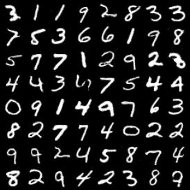
Low-Rank Structure of NFK. Motivated by the Manifold Hypothesis of Data that it is widely believed that real world high dimensional data lives in a low dimensional manifold (Roweis and Saul, 2000, Rifai et al., 2011a; b), we investigate the structure of NFKs and present empirical evidence that NFKs of good models have low-rank spectral structure. Firstly, we start by examining supervised learning models. We study the spectrum structure of the empirical NFK of trained neural networks with different architectures. We trained a LeNet-5 (LeCun et al., 1998) CNN and a 3-layer MLP network by minimizing binary cross entropy loss, and then compute the eigen-decomposition of the NFK Gram matrix. We show the explained ratio plot in Figure 2. We see that the spectrum of CNN NTK concentrates on fewer large eigenvalues, thus exhibiting a lower effective-rank structure compared to the MLP, which can be explained by the fact that CNN has better model inductive bias for image data domain. For unsupervised learning models, we trained a small unconditional DCGAN (Radford et al., 2016) model on MNIST dataset. We compare the results of a fully trained model against a randomly initialized model in Fig. 2 (note the logarithm scale of the $x$ -axis). Remarkably, the trained model demonstrates an extreme degree of low-rankness that top $100$ principle components explain over $99.5\%$ of the overall variance, where $100$ is two orders of magnitude smaller than both number of examples and number of parameters in the discriminator. We include more experimental results and discussions in appendix due to the space constraints.

Efficient Low-Rank Approximation of NFK. The theoretical insights and empirical evidence presented above hint at a natural solution to address the challenge of high-dimensionality of $V_{{\mathbf{x}}}\in\mathbb{R}^{|{\bm{\theta}}|}$ : we can turn to seek a low-rank approximation to the NFK. According to the Mercer’s theorem (Mercer, 1909), for positive definite kernel $\mathcal{K}({\mathbf{x}},{\mathbf{z}})=\langle\varphi({\mathbf{x}}),\varphi({\mathbf{z}})\rangle$ we have $\mathcal{K}({\mathbf{x}},{\mathbf{z}})=\sum_{i=1}^{\infty}\lambda_{i}\phi_{i}({\mathbf{x}})\phi_{i}({\mathbf{z}}),\;{\mathbf{x}},{\mathbf{z}}\in\mathcal{X}$ , where $\left\{\left(\lambda_{i},\phi_{i}\right)\right\}$ are the eigenvalues and eigenfunctions of the kernel $\mathcal{K}$ , with respect to the integral operator $\int p({\mathbf{z}}){\mathcal{K}}({\mathbf{x}},{\mathbf{z}})\phi_{i}({\mathbf{z}})\differential{{\mathbf{z}}}=\lambda_{i}\phi_{i}({\mathbf{x}})$ . The linear feature embedding representation $\varphi({\mathbf{x}})$ can thus be constructed from the orthonormal eigen-basis $\left\{\left(\lambda_{i},\phi_{i}\right)\right\}$ as $\varphi({\mathbf{x}})\equiv\left[\sqrt{\lambda_{1}}\phi_{1}({\mathbf{x}}),\sqrt{\lambda_{2}}\phi_{2}({\mathbf{x}}),\ldots\right]\equiv\left[\sqrt{\lambda_{i}}\phi_{i}({\mathbf{x}})\right],\;i=1,\ldots,\infty$ . To obtain a low-rank approximation, we only keep top- $k$ largest eigen-basis $\left\{\left(\lambda_{i},\phi_{i}\right)\right\}$ ordered by corresponding eigenvalues $\lambda_{i}$ to form the low-rank $k$ -dimensional feature embedding ${\mathbf{e}}({\mathbf{x}})\in\mathbb{R}^{k}$ , $k\ll N,k\ll|{\bm{\theta}}|$

{\mathbf{e}}({\mathbf{x}})\equiv\left[\sqrt{\lambda_{1}}\phi_{1}({\mathbf{x}}),\sqrt{\lambda_{2}}\phi_{2}({\mathbf{x}}),\ldots\sqrt{\lambda_{k}}\phi_{k}({\mathbf{x}})\right]\equiv\left[\sqrt{\lambda_{i}}\phi_{i}({\mathbf{x}})\right],\;i=1,\ldots,k

(4)

By applying our proposed NFK formulation $\mathcal{K}_{\mathrm{nfk}}$ to pre-trained neural network model $f({\mathbf{x}};{\bm{\theta}})$ , we can obtain a compact low-dimensional feature representation ${\mathbf{e}}_{\mathrm{nfk}}({\mathbf{x}})\in\mathbb{R}^{k}$ in this way. We call it the low-rank NFK feature embedding.

We then illustrate how to estimate the eigenvalues and eigenfunctions of NFK $\mathcal{K}_{\mathrm{nfk}}$ from data. Given dataset ${\mathcal{D}}$ , the Gram matrix ${\mathbf{K}}\in\mathbb{R}^{N\times N}$ of kernel $\mathcal{K}$ is defined as ${\mathbf{K}}({\mathbf{x}}_{i},{\mathbf{x}}_{j})=\mathcal{K}({\mathbf{x}}_{i},{\mathbf{x}}_{j})$ . We use ${\mathbf{X}}\equiv\left[{\mathbf{x}}_{i}\right]_{i=1}^{N}$ to denote the matrix of all data examples, and use $\phi_{i}({\mathbf{X}})\in\mathbb{R}^{N}$ to denote the concatenated vector of evaluating $i$ -th eigenfunction $\phi_{i}$ at all data examples. Then by performing eigen-decomposition of the Gram matrix ${\mathbf{K}}={\mathbf{\Phi}}\texttt{diag}(\Lambda){\mathbf{\Phi}}^{\top}$ , the $i$ -th eigenvector ${\mathbf{\Phi}}_{i}\in\mathbb{R}^{N}$ and eigenvalue $\Lambda_{i}$ can be seen as unbiased estimation of the $i$ -th eigenfunction $\phi_{i}$ and eigenvalue $\lambda_{i}$ of the kernel ${\mathcal{K}}$ , evaluated at training data examples ${\mathbf{X}}$ , $\phi_{i}\left({\mathbf{X}}\right)\approx\sqrt{N}{\mathbf{\Phi}}_{i},\lambda_{i}\approx\frac{1}{N}\Lambda_{i}$ . Based on these estimations, we can thus approximate the eigenfunction $\phi_{i}$ via the integral operator by Monte-Carlo estimation with empirical data distribution,

\lambda_{i}\phi_{i}({\mathbf{x}})=\int p({\mathbf{z}}){\mathcal{K}}({\mathbf{x}},{\mathbf{z}})\phi_{i}({\mathbf{z}})\differential{{\mathbf{z}}}\approx\mathbb{E}_{{\mathbf{x}}_{j}\in p_{\mathrm{data}}}\mathcal{K}({\mathbf{x}},{\mathbf{x}}_{j})\phi_{j}({\mathbf{x}}_{j})\approx\frac{1}{N}\sum_{j=1}^{N}\mathcal{K}({\mathbf{x}},{\mathbf{x}}_{j}){\mathbf{\Phi}}_{ji}

(5)

Given new test data example ${\mathbf{x}}^{\star}$ , we can now approximate the eigenfunction evaluation $\phi_{i}({\mathbf{x}}^{\star})$ by the projection of kernel function evaluation results centered on training data examples $\mathcal{K}({\mathbf{x}}^{\star},{\mathbf{X}})\equiv\left[\mathcal{K}({\mathbf{x}}^{\star},{\mathbf{x}}_{j})\right]_{j=1}^{N}$ onto the $i$ -th eigenvector ${\mathbf{\Phi}}_{i}$ of kernel Gram matrix ${\mathbf{K}}$ . We adopt this method as the baseline approach for low-rank approximation, and present the baseline algorithm description in Alg. 1.

However, due to the fact that it demands explicit computation and manipulation of the Fisher vector matrix ${\mathbf{V}}\in\mathbb{R}^{N\times|{\bm{\theta}}|}$ and the Gram matrix ${\mathbf{K}}\in\mathbb{R}^{N\times N}$ in Alg. 1, straightforward application of the baseline approach, as well as other off-the-shelf classical kernel approximation (Williams and Seeger, 2000, Rahimi and Recht, 2007) and SVD methods (Halko et al., 2011), are practically infeasible to scale to larger-scale machine learning settings, where both the number of data examples $N$ and the number of model parameters $|{\bm{\theta}}|$ can be extremely large.

To tackle the posed scalability issue, we propose a novel highly efficient and scalable algorithm for computing low-rank approximation of NFK. Given dataset ${\mathcal{D}}$ and model $f({\mathbf{x}};{\bm{\theta}})$ , We aim to compute the truncated SVD of the Fisher vector matrix ${\mathbf{V}}={\mathbf{\Phi}}\texttt{diag}(\Sigma){\mathbf{P}}^{\top},{\mathbf{P}}\in\mathbb{R}^{|{\bm{\theta}}|\times k}$ . Based on the idea of power methods (Golub and Van der Vorst, 2000, Bathe, 1971) for finding leading top eigenvectors, we start from a random vector ${\mathbf{v}}_{0}$ and iteratively construct the sequence ${\mathbf{v}}_{t+1}=\frac{{\mathbf{V}}{\mathbf{V}}^{\top}{\mathbf{v}}_{t}}{\|{\mathbf{V}}{\mathbf{V}}^{\top}{\mathbf{v}}_{t}\|}$ . By leveraging the special structure of ${\mathbf{V}}$ that it can be obtained from the Jacobian matrix $J_{{\bm{\theta}}}(\mathbf{X})\in\mathbb{R}^{N\times|{\bm{\theta}}|}$ up to element-wise linear transformation under the NFK formulation in Sec. 3, we can decompose each iterative step into a Jacobian Vector Product (JVP) and a Vector Jacobian Product (VJP). With modern automatic-differentiation techniques, we can evaluate both JVP and VJP efficiently, which only requires the same order of computational costs of one vanilla backward-pass and forward-pass of neural networks respectively. With computed truncated SVD results, we can approximate the projection term in Eq. 5 by $\mathcal{K}\left(\mathbf{x},\mathbf{X}\right)^{\top}{\mathbf{\Phi}}_{i}=V_{{\mathbf{x}}}{\mathbf{V}}^{\top}{\mathbf{\Phi}}_{i}\approx V_{{\mathbf{x}}}\texttt{diag}(\Sigma_{i}){\mathbf{P}}_{i}$ , which is again in the JVP form so that we can pre-compute and store the truncated SVD results and evaluate the eigenfunction of any test data example via one efficient JVP forward-pass. We describe our proposed algorithm briefly in Alg. 2.

{\mathbf{V}}={\mathbf{\Phi}}\texttt{diag}(\Sigma){\mathbf{P}}^{\top},{\mathbf{P}}\in\mathbb{R}^{|{\bm{\theta}}|\times k}

using power iteration methods via JVP/VJP evaluations

2:compute

\mathcal{K}\left(\mathbf{x},\mathbf{X}\right)^{\top}{\mathbf{\Phi}}_{i}\approx V_{{\mathbf{x}}}\texttt{diag}(\Sigma_{i}){\mathbf{P}}_{i}

via JVP evaluation

3:obtain

{\mathbf{e}}_{\mathrm{nfk}}({\mathbf{x}}^{*})\in\mathbb{R}^{k}

via Eq. 5 and Eq. 4

Algorithm 2 Our proposed method: compute low-rank NFK feature embedding

4 Experiments

In this section, we evaluate NFK in the following settings. We first evaluate the proposed low-rank kernel approximation algorithm (Sec. 3.2), in terms of both approximation accuracy and running time efficiency. Next, we evaluate NFK on various representation learning tasks in both supervised, semi-supervised and unsupervised learning settings.

4.1 Quality and Efficiency of Low-rank NFK Approximations

We implement our proposed low-rank kernel approximation algorithm in Jax (Bradbury et al., 2018) with distributed multi-GPU parallel computation support. For the baseline methods for comparison, we first compute the full kernel Gram matrix using the neural-tangets (Novak et al., 2020) library, and then use sklearn.decomposition.TruncatedSVD to obtain the truncated SVD results. All model and algorithm hyper-parameters are included in the Appendix.

Computational Costs. We start by comparing running time costs of computing top NFK eigen-vectors via truncated SVD. We use two models for the comparison, a DCGAN-like GAN model in (Zhai et al., 2019) and a Wide ResNet (WRN) with $40$ layers and $2$ times wider than original network (denoted as WRN- $40$ - $2$ ). Please see appendix for the detailed description of hyper-parameters. We observed that our proposed algorithm could achieve nearly linear time scaling, while the baseline method would not be able to handle more than $2^{14}$ data examples as the memory usage and time complexity are too high to afford. We also see in Fig. 3 that by utilizing multi-GPU parallelism, we achieved further speed-up which scales almost linearly with the number of GPUs. We emphasize that given the number of desired eigenvectors, the time complexity of our method scales linearly with the number of data examples and the demanded memory usage remains constant with adequate data batch size, since explicit computation and storage of the full kernel matrix is never needed.

Approximation accuracy. We investigate the approximation error of our proposed low-rank approximation method. Since we did not introduce any additional approximations, our method shares the same approximation error bound with the existing randomized SVD algorithm (Martinsson and Tropp, 2020, Halko et al., 2011) and would only expect differences compared to the baseline randomized SVD algorithm up to numerical errors. To evaluate the quality of the low-rank kernel approximation, we use LeNet-5 and compute its full NFK Gram matrix on MNIST dataset. Please see appendix for detailed hyper-parameter setups. We show in Fig. 3 the approximation errors of top- $128$ eigenvalues along with corresponding explained variances. We obtain less than $1e-8$ absolute error and less than $1e-7$ relative error in top eigen-modes which explains most of the data.

Table 1: CIFAR-10 accuracies of linear evaluation on top of representations learned with unsupervised and self-supervised methods. NFK-128d denotes the 128 dimensional embeddings from the low-rank approximation of the NFK (ie AFV). Remarkably, we can use 128 dimensions to exactly recover the performance of the 5.9M dimensional Fisher Vectors.

Model	Acc	Category	#Features
Examplar CNN (Dosovitskiy et al., 2015)	$84.3$	Unsupervised	-
BiGAN (Mu et al., 2020)	$70.5$	Unsupervised	-
RotNet Linear (Gidaris et al., 2018)	$81.8$	Self-Supervised	$\sim 25$ K
AET Linear (Zhang et al., 2019)	$83.3$	Self-Supervised	$\sim 25$ K
VAE(Mu et al., 2020)	$61.5$	Unsupervised	-
VAE-NFK-128d (ours)	$63.2$	Unsupervised	$\mathbf{128}$
VAE-NFK-256d (ours)	$68.7$	Unsupervised	$\mathbf{256}$
GAN-Supervised	$92.7$	Supervised	-
GAN-Activations	$65.3$	Unsupervised	-
GAN-AFV (Zhai et al., 2019)	$89.1$	Unsupervised	5.9M
GAN-AFV (re-implementation) (Zhai et al., 2019)	$89.8$	Unsupervised	5.9M
GAN-NFK-128d (ours)	$\mathbf{89.8}$	Unsupervised	$\mathbf{128}$
GAN-NFK-256d (ours)	$\mathbf{89.8}$	Unsupervised	$\mathbf{256}$

4.2 Low-rank NFK Embedding as Data Representations

In this section we evaluate NFK to answer the following: Q1. In line with the question raised in Sec. 1, how does our proposed low-rank NFK embedding differ from the intermediate layer activations for data representation? Q2. How does the low-rank NFK embedding compare to simply using gradients (Jacobians) as data representation? Q3. To what extent can the low-rank NFK embedding preserve the information in full Fisher vector? Q4. Does the NFK embedding representation lead to better generalization performance in terms of better sample efficiency and faster adaptation? We conduct comparative studies on different tasks to understand the NFK embedding and present empirical observations to answer these questions in following sections.

NFK Representations from Unsupervised Generative Models. In order to examine the effectiveness of the low-rank NFK embeddings as data representations in unsupervised learning setting, we consider GANs and VAEs as representative generative models and compute the low-rank NFK embeddings. Then we adopt the linear probing protocol by training a linear classifier on top of the obtained embeddings and report the classification performance to quantify the quality of NFK data representation. For GANs, we use the same pretrained GAN model from (Zhai et al., 2019) and reimplemented the AFV baseline. For VAEs, we follow the same model architecture proposed in (Child, 2020). We then apply the proposed truncated SVD algorithm with $10$ power iterations to obtain the $256$ dimensional embedding via projection. We present our results on CIFAR-10 (Krizhevsky et al., 2009a) in Table. 1. We use GAN-NFK-128d (GAN-NFK-256d) to denote the NFK embedding obtained from using top- $128$ (top- $256$ ) eigenvectors in our GAN model. Our VAE models (VAE-NFK-128d and VAE-NFK-256d) follow the same notations. For VAE baselines, the method proposed in (Mu et al., 2020) combines both gradients features and activations-based features into one linear model, denoted as VAE in the table. For GAN baselines, we first consider using intermediate layer activations only as data representation, referred to as the GAN-Activations model. We then consider using full Fisher vector as representation, namely using the normalized gradients w.r.t all model parameters as features, denoted as the GAN-AFV model as proposed in (Zhai et al., 2019). Moreover, we also compare our results against training whole neural network using data labels in a supervised learning way, denoted as GAN-Supervised model.

As shown in Table. 1, by contrasting against the baseline GAN-AFV from GAN-Activations, as well as validation in recent works (Zhai et al., 2019, Mu et al., 2020), gradients provide additional useful information beyond layer activations based features. However, it would be impractical to use all gradients or full Fisher vector as representation when scaling up to large-scale neural network models. For example, VAE (Child, 2020) has $\sim 40M$ parameters, it would not be possible to apply the baseline methods directly. Our proposed low-rank NFK embedding approach addressed this challenge by building low-dim vector representation from efficient kernel approximation algorithm, making it possible to utilize all model parameters’ gradients information by embedding it into a low-dim vector, e.g. $256$ -dimensional embedding in VAE-NFK-256d from $\sim 40M$ parameters. As our low-rank NFK embedding is obtained by linear projections of full Fisher vectors, it naturally provides answers for Q2 that the NFK embedding can be viewed as a compact yet informative representation containing information from all gradients. We see from Table. 1 that by using top- $128$ eigenvectors, the low-rank NFK embedding is able to recover the performance of full $\sim 5.9M$ -dimension Fisher vector, which provides positive evidence for Q3 that we can preserve most of the useful information in Fisher vector by taking advantage of the low-rank structure of NFK spectrum.

Table 2: Error rates of semi-supervised classification on CIFAR10 and SVHN, varying labels from 500 to 4000. NFK-128d yields extremely competitive performance, compared to other more sophisticated baselines, Mixup (Zhang et al., 2018), VAT (Miyato et al., 2019), MeanTeacher(Tarvainen and Valpola, 2017), MixMatch (Berthelot et al., 2019), Improved GAN(Salimans et al., 2016), all are jointly learns with labels, . Also note that the architecture used by MixMatch yields a 4.13% supervised learning error rate, which is a much stronger than our supervised baseline (7.3%).

Model	Category	CIFAR-10				SVHN
		$500$	$1000$	$2000$	$4000$	$500$	$1000$	$2000$	$4000$
Mixup	Joint	$36.17$	$25.72$	$18.14$	$13.15$	$29.62$	$16.79$	$10.47$	$7.96$
VAT	Joint	$26.11$	$18.68$	$14.40$	$11.05$	$7.44$	$5.98$	$4.85$	$4.20$
MeanTeacher	Joint	$47.32$	$42.01$	$17.32$	$12.17$	$6.45$	$3.82$	$3.75$	$3.51$
MixMatch	Joint	$9.65$	$7.75$	$7.03$	$6.24$	$3.64$	$3.27$	$3.04$	$2.89$
Improved GAN	Joint	-	$19.22$	$17.25$	$15.59$	$18.44$	$8.11$	$6.16$	-
NFK-128d (ours)	Pretrained	$20.68$	$14.77$	$13.82$	$12.95$	$8.74$	$4.47$	$3.82$	$3.19$

NFK Representations for Semi-Supervised Learning. We then test the low-rank NFK embeddings in the semi-supervised learning setting. Following the standard semi-supervised learning benchmark settings (Berthelot et al., 2019, Miyato et al., 2019, Laine and Aila, 2017, Sajjadi et al., 2016, Tarvainen and Valpola, 2017), we evaluate our method on CIFAR-10 (Krizhevsky et al., 2009a) and SVHN datasets (Krizhevsky et al., 2009b). We treat most of the dataset as unlabeled data and use few examples as labeled data. We use the same GAN model as the unsupervised learning setting above, and compute top- $128$ eigenvectors using training dataset (labeled and unlabeled) to derive the $128$ -dimensional NFK embedding. Then we only use the labeled data to train a linear classifier on top of the NFK embedding features, denoted as the NFK-128d model. We vary the number of labeled training examples and report the results in Table. 2, in comparison with other baseline methods. We see that NFK-128d achieves very competitive performance. On CIFAR-10, NFK-128d is only outperformed by the state-of-the-art semi-supervised learning algorithm MixMatch (Berthelot et al., 2019), which also uses a stronger architecture than ours. The results on SVHN are mixed though NFK-128d is competitive with the top performing approaches. The results demonstrated the effectiveness of NFK embeddings from unsupervised generative models in semi-supervised learning, showing promising sample efficiency for Q4.

Table 3: Supervised knowledge distillation results (classification accuracy on test dataset) on CIFAR10 against baseline methods KD (Hinton et al., 2015), FitNet (Romero et al., 2015), AT (Zagoruyko and Komodakis, 2017), NST (Huang and Wang, 2017), VID-I (Ahn et al., 2019), numbers are from (Ahn et al., 2019).

	Teacher	Student	KD	FitNet	AT	NST	VID-I	NFKD (ours)
ACC	$94.26$	$90.72$	$91.27$	$90.64$	$91.60$	$91.16$	$91.85$	$\mathbf{92.42}$

NFK Representations for Knowledge Distillation. We next test the effectiveness of using low-rank NFK embedding for knowledge distillation in the supervised learning setting. We include more details of the distillation method in the Appendix. Our experiments are conducted on CIFAR10, with a teacher set as the WRN-40-2 model and student being WRN-16-1. After training the teacher, we compute the low-rank approximation of NFK of the teacher model, using top- $20$ eigenvectors. We include more details about the distillation method setup in the Appendix. Our results are reported in Table. 3. We see that our method achieves superior results compared to other competitive baseline knowledge distillation methods, which mainly use the logits and activations from teacher network as distillation target.

5 Conclusions

In this work, we propose a novel principled approach to representation extraction from pre-trained neural network models. We introduce NFK by extending the Fisher kernel to neural networks in both unsupervised learning and superevised learning settings, and propose a novel low-rank kernel approximation algorithm, which allows us to obtain a compact feature representation in a highly efficient and scalable way.

References

Jaakkola and Haussler (1998) Tommi S. Jaakkola and David Haussler. Exploiting generative models in discriminative classifiers. In Michael J. Kearns, Sara A. Solla, and David A. Cohn, editors, Advances in Neural Information Processing Systems 11, [NIPS Conference, Denver, Colorado, USA, November 30 - December 5, 1998], pages 487–493. The MIT Press, 1998. URL http://papers.nips.cc/paper/1520-exploiting-generative-models-in-discriminative-classifiers.
He et al. (2016) Kaiming He, Xiangyu Zhang, Shaoqing Ren, and Jian Sun. Deep residual learning for image recognition. In 2016 IEEE Conference on Computer Vision and Pattern Recognition, CVPR 2016, Las Vegas, NV, USA, June 27-30, 2016, pages 770–778. IEEE Computer Society, 2016. doi: 10.1109/CVPR.2016.90. URL https://doi.org/10.1109/CVPR.2016.90.
Hinton et al. (2015) Geoffrey E. Hinton, Oriol Vinyals, and Jeffrey Dean. Distilling the knowledge in a neural network. CoRR, abs/1503.02531, 2015. URL http://arxiv.org/abs/1503.02531.
Goodfellow et al. (2014) Ian J Goodfellow, Jean Pouget-Abadie, Mehdi Mirza, Bing Xu, David Warde-Farley, Sherjil Ozair, Aaron Courville, and Yoshua Bengio. Generative adversarial networks. arXiv preprint arXiv:1406.2661, 2014. URL https://arxiv.org/abs/1406.2661.
Kingma and Welling (2014) Diederik P. Kingma and Max Welling. Auto-encoding variational bayes. In Yoshua Bengio and Yann LeCun, editors, 2nd International Conference on Learning Representations, ICLR 2014, Banff, AB, Canada, April 14-16, 2014, Conference Track Proceedings, 2014. URL http://arxiv.org/abs/1312.6114.
Chen et al. (2020a) Mark Chen, Alec Radford, Rewon Child, Jeffrey Wu, Heewoo Jun, David Luan, and Ilya Sutskever. Generative pretraining from pixels. In Proceedings of the 37th International Conference on Machine Learning, ICML 2020, 13-18 July 2020, Virtual Event, volume 119 of Proceedings of Machine Learning Research, pages 1691–1703. PMLR, 2020a. URL http://proceedings.mlr.press/v119/chen20s.html.
Mu et al. (2020) Fangzhou Mu, Yingyu Liang, and Yin Li. Gradients as features for deep representation learning. In 8th International Conference on Learning Representations, ICLR 2020, Addis Ababa, Ethiopia, April 26-30, 2020. OpenReview.net, 2020. URL https://openreview.net/forum?id=BkeoaeHKDS.
Jacot et al. (2018) Arthur Jacot, Clément Hongler, and Franck Gabriel. Neural tangent kernel: Convergence and generalization in neural networks. In Samy Bengio, Hanna M. Wallach, Hugo Larochelle, Kristen Grauman, Nicolò Cesa-Bianchi, and Roman Garnett, editors, Advances in Neural Information Processing Systems 31: Annual Conference on Neural Information Processing Systems 2018, NeurIPS 2018, December 3-8, 2018, Montréal, Canada, pages 8580–8589, 2018. URL https://proceedings.neurips.cc/paper/2018/hash/5a4be1fa34e62bb8a6ec6b91d2462f5a-Abstract.html.
Hofmann et al. (2008) Thomas Hofmann, Bernhard Schölkopf, and Alexander J Smola. Kernel methods in machine learning. The annals of statistics, pages 1171–1220, 2008.
Neal (1996) Radford M Neal. Priors for infinite networks. In Bayesian Learning for Neural Networks, pages 29–53. Springer, 1996.
Williams (1996) Christopher K. I. Williams. Computing with infinite networks. In Michael Mozer, Michael I. Jordan, and Thomas Petsche, editors, Advances in Neural Information Processing Systems 9, NIPS, Denver, CO, USA, December 2-5, 1996, pages 295–301. MIT Press, 1996. URL http://papers.nips.cc/paper/1197-computing-with-infinite-networks.
Roux and Bengio (2007) Nicolas Le Roux and Yoshua Bengio. Continuous neural networks. In Marina Meila and Xiaotong Shen, editors, Proceedings of the Eleventh International Conference on Artificial Intelligence and Statistics, AISTATS 2007, San Juan, Puerto Rico, March 21-24, 2007, volume 2 of JMLR Proceedings, pages 404–411. JMLR.org, 2007. URL http://proceedings.mlr.press/v2/leroux07a.html.
Hazan and Jaakkola (2015) Tamir Hazan and Tommi S. Jaakkola. Steps toward deep kernel methods from infinite neural networks. CoRR, abs/1508.05133, 2015. URL http://arxiv.org/abs/1508.05133.
Lee et al. (2018) Jaehoon Lee, Yasaman Bahri, Roman Novak, Samuel S. Schoenholz, Jeffrey Pennington, and Jascha Sohl-Dickstein. Deep neural networks as gaussian processes. In 6th International Conference on Learning Representations, ICLR 2018, Vancouver, BC, Canada, April 30 - May 3, 2018, Conference Track Proceedings. OpenReview.net, 2018. URL https://openreview.net/forum?id=B1EA-M-0Z.
de G. Matthews et al. (2018) Alexander G. de G. Matthews, Jiri Hron, Mark Rowland, Richard E. Turner, and Zoubin Ghahramani. Gaussian process behaviour in wide deep neural networks. In 6th International Conference on Learning Representations, ICLR 2018, Vancouver, BC, Canada, April 30 - May 3, 2018, Conference Track Proceedings. OpenReview.net, 2018. URL https://openreview.net/forum?id=H1-nGgWC-.
Chen and Xu (2021) Lin Chen and Sheng Xu. Deep neural tangent kernel and laplace kernel have the same RKHS. In 9th International Conference on Learning Representations, ICLR 2021, Virtual Event, Austria, May 3-7, 2021. OpenReview.net, 2021. URL https://openreview.net/forum?id=vK9WrZ0QYQ.
Geifman et al. (2020) Amnon Geifman, Abhay Kumar Yadav, Yoni Kasten, Meirav Galun, David W. Jacobs, and Ronen Basri. On the similarity between the laplace and neural tangent kernels. In Hugo Larochelle, Marc’Aurelio Ranzato, Raia Hadsell, Maria-Florina Balcan, and Hsuan-Tien Lin, editors, Advances in Neural Information Processing Systems 33: Annual Conference on Neural Information Processing Systems 2020, NeurIPS 2020, December 6-12, 2020, virtual, 2020. URL https://proceedings.neurips.cc/paper/2020/hash/1006ff12c465532f8c574aeaa4461b16-Abstract.html.
Belkin et al. (2018) Mikhail Belkin, Siyuan Ma, and Soumik Mandal. To understand deep learning we need to understand kernel learning. In Jennifer G. Dy and Andreas Krause, editors, Proceedings of the 35th International Conference on Machine Learning, ICML 2018, Stockholmsmässan, Stockholm, Sweden, July 10-15, 2018, volume 80 of Proceedings of Machine Learning Research, pages 540–548. PMLR, 2018. URL http://proceedings.mlr.press/v80/belkin18a.html.
Ghorbani et al. (2020) Behrooz Ghorbani, Song Mei, Theodor Misiakiewicz, and Andrea Montanari. When do neural networks outperform kernel methods? In Hugo Larochelle, Marc’Aurelio Ranzato, Raia Hadsell, Maria-Florina Balcan, and Hsuan-Tien Lin, editors, Advances in Neural Information Processing Systems 33: Annual Conference on Neural Information Processing Systems 2020, NeurIPS 2020, December 6-12, 2020, virtual, 2020. URL https://proceedings.neurips.cc/paper/2020/hash/a9df2255ad642b923d95503b9a7958d8-Abstract.html.
Daniely et al. (2016) Amit Daniely, Roy Frostig, and Yoram Singer. Toward deeper understanding of neural networks: The power of initialization and a dual view on expressivity. In Daniel D. Lee, Masashi Sugiyama, Ulrike von Luxburg, Isabelle Guyon, and Roman Garnett, editors, Advances in Neural Information Processing Systems 29: Annual Conference on Neural Information Processing Systems 2016, December 5-10, 2016, Barcelona, Spain, pages 2253–2261, 2016. URL https://proceedings.neurips.cc/paper/2016/hash/abea47ba24142ed16b7d8fbf2c740e0d-Abstract.html.
Perronnin and Dance (2007) Florent Perronnin and Christopher R. Dance. Fisher kernels on visual vocabularies for image categorization. In 2007 IEEE Computer Society Conference on Computer Vision and Pattern Recognition (CVPR 2007), 18-23 June 2007, Minneapolis, Minnesota, USA. IEEE Computer Society, 2007. doi: 10.1109/CVPR.2007.383266. URL https://doi.org/10.1109/CVPR.2007.383266.
Dinh et al. (2015) Laurent Dinh, David Krueger, and Yoshua Bengio. NICE: non-linear independent components estimation. In Yoshua Bengio and Yann LeCun, editors, 3rd International Conference on Learning Representations, ICLR 2015, San Diego, CA, USA, May 7-9, 2015, Workshop Track Proceedings, 2015. URL http://arxiv.org/abs/1410.8516.
van den Oord et al. (2016) Aäron van den Oord, Nal Kalchbrenner, and Koray Kavukcuoglu. Pixel recurrent neural networks. In Maria-Florina Balcan and Kilian Q. Weinberger, editors, Proceedings of the 33nd International Conference on Machine Learning, ICML 2016, New York City, NY, USA, June 19-24, 2016, volume 48 of JMLR Workshop and Conference Proceedings, pages 1747–1756. JMLR.org, 2016. URL http://proceedings.mlr.press/v48/oord16.html.
Salakhutdinov (2014) Ruslan Salakhutdinov. Deep learning. In Sofus A. Macskassy, Claudia Perlich, Jure Leskovec, Wei Wang, and Rayid Ghani, editors, The 20th ACM SIGKDD International Conference on Knowledge Discovery and Data Mining, KDD ’14, New York, NY, USA - August 24 - 27, 2014, page 1973. ACM, 2014. doi: 10.1145/2623330.2630809. URL https://doi.org/10.1145/2623330.2630809.
Achille et al. (2019) Alessandro Achille, Michael Lam, Rahul Tewari, Avinash Ravichandran, Subhransu Maji, Charless C. Fowlkes, Stefano Soatto, and Pietro Perona. Task2vec: Task embedding for meta-learning. In 2019 IEEE/CVF International Conference on Computer Vision, ICCV 2019, Seoul, Korea (South), October 27 - November 2, 2019, pages 6429–6438. IEEE, 2019. doi: 10.1109/ICCV.2019.00653. URL https://doi.org/10.1109/ICCV.2019.00653.
Dai et al. (2017) Zihang Dai, Amjad Almahairi, Philip Bachman, Eduard H. Hovy, and Aaron C. Courville. Calibrating energy-based generative adversarial networks. In 5th International Conference on Learning Representations, ICLR 2017, Toulon, France, April 24-26, 2017, Conference Track Proceedings. OpenReview.net, 2017. URL https://openreview.net/forum?id=SyxeqhP9ll.
Zhai et al. (2019) Shuangfei Zhai, Walter Talbott, Carlos Guestrin, and Joshua M. Susskind. Adversarial fisher vectors for unsupervised representation learning. In Hanna M. Wallach, Hugo Larochelle, Alina Beygelzimer, Florence d’Alché-Buc, Emily B. Fox, and Roman Garnett, editors, Advances in Neural Information Processing Systems 32: Annual Conference on Neural Information Processing Systems 2019, NeurIPS 2019, December 8-14, 2019, Vancouver, BC, Canada, pages 11156–11166, 2019. URL https://proceedings.neurips.cc/paper/2019/hash/7e1cacfb27da22fb243ff2debf4443a0-Abstract.html.
Che et al. (2020) Tong Che, Ruixiang Zhang, Jascha Sohl-Dickstein, Hugo Larochelle, Liam Paull, Yuan Cao, and Yoshua Bengio. Your GAN is secretly an energy-based model and you should use discriminator driven latent sampling. In Hugo Larochelle, Marc’Aurelio Ranzato, Raia Hadsell, Maria-Florina Balcan, and Hsuan-Tien Lin, editors, Advances in Neural Information Processing Systems 33: Annual Conference on Neural Information Processing Systems 2020, NeurIPS 2020, December 6-12, 2020, virtual, 2020. URL https://proceedings.neurips.cc/paper/2020/hash/90525e70b7842930586545c6f1c9310c-Abstract.html.
Burda et al. (2016) Yuri Burda, Roger B. Grosse, and Ruslan Salakhutdinov. Importance weighted autoencoders. In Yoshua Bengio and Yann LeCun, editors, 4th International Conference on Learning Representations, ICLR 2016, San Juan, Puerto Rico, May 2-4, 2016, Conference Track Proceedings, 2016. URL http://arxiv.org/abs/1509.00519.
Grathwohl et al. (2020) Will Grathwohl, Kuan-Chieh Wang, Jörn-Henrik Jacobsen, David Duvenaud, Mohammad Norouzi, and Kevin Swersky. Your classifier is secretly an energy based model and you should treat it like one. In 8th International Conference on Learning Representations, ICLR 2020, Addis Ababa, Ethiopia, April 26-30, 2020. OpenReview.net, 2020. URL https://openreview.net/forum?id=Hkxzx0NtDB.
Roweis and Saul (2000) Sam T Roweis and Lawrence K Saul. Nonlinear dimensionality reduction by locally linear embedding. science, 290(5500):2323–2326, 2000.
Rifai et al. (2011a) Salah Rifai, Pascal Vincent, Xavier Muller, Xavier Glorot, and Yoshua Bengio. Contractive auto-encoders: Explicit invariance during feature extraction. In Lise Getoor and Tobias Scheffer, editors, Proceedings of the 28th International Conference on Machine Learning, ICML 2011, Bellevue, Washington, USA, June 28 - July 2, 2011, pages 833–840. Omnipress, 2011a. URL https://icml.cc/2011/papers/455_icmlpaper.pdf.
Rifai et al. (2011b) Salah Rifai, Yann N. Dauphin, Pascal Vincent, Yoshua Bengio, and Xavier Muller. The manifold tangent classifier. In John Shawe-Taylor, Richard S. Zemel, Peter L. Bartlett, Fernando C. N. Pereira, and Kilian Q. Weinberger, editors, Advances in Neural Information Processing Systems 24: 25th Annual Conference on Neural Information Processing Systems 2011. Proceedings of a meeting held 12-14 December 2011, Granada, Spain, pages 2294–2302, 2011b. URL https://proceedings.neurips.cc/paper/2011/hash/d1f44e2f09dc172978a4d3151d11d63e-Abstract.html.
LeCun et al. (1998) Yann LeCun, Léon Bottou, Yoshua Bengio, and Patrick Haffner. Gradient-based learning applied to document recognition. Proceedings of the IEEE, 86(11):2278–2324, 1998.
Radford et al. (2016) Alec Radford, Luke Metz, and Soumith Chintala. Unsupervised representation learning with deep convolutional generative adversarial networks. In Yoshua Bengio and Yann LeCun, editors, 4th International Conference on Learning Representations, ICLR 2016, San Juan, Puerto Rico, May 2-4, 2016, Conference Track Proceedings, 2016. URL http://arxiv.org/abs/1511.06434.
Mercer (1909) J Mercer. Functions ofpositive and negativetypeand theircommection with the theory ofintegral equations. Philos. Trinsdictions Rogyal Soc, 209:4–415, 1909.
Williams and Seeger (2000) Christopher K. I. Williams and Matthias W. Seeger. Using the nyström method to speed up kernel machines. In Todd K. Leen, Thomas G. Dietterich, and Volker Tresp, editors, Advances in Neural Information Processing Systems 13, Papers from Neural Information Processing Systems (NIPS) 2000, Denver, CO, USA, pages 682–688. MIT Press, 2000. URL https://proceedings.neurips.cc/paper/2000/hash/19de10adbaa1b2ee13f77f679fa1483a-Abstract.html.
Rahimi and Recht (2007) Ali Rahimi and Benjamin Recht. Random features for large-scale kernel machines. In John C. Platt, Daphne Koller, Yoram Singer, and Sam T. Roweis, editors, Advances in Neural Information Processing Systems 20, Proceedings of the Twenty-First Annual Conference on Neural Information Processing Systems, Vancouver, British Columbia, Canada, December 3-6, 2007, pages 1177–1184. Curran Associates, Inc., 2007. URL https://proceedings.neurips.cc/paper/2007/hash/013a006f03dbc5392effeb8f18fda755-Abstract.html.
Halko et al. (2011) Nathan Halko, Per-Gunnar Martinsson, and Joel A. Tropp. Finding structure with randomness: Probabilistic algorithms for constructing approximate matrix decompositions. SIAM Rev., 53(2):217–288, 2011. doi: 10.1137/090771806. URL https://doi.org/10.1137/090771806.
Golub and Van der Vorst (2000) Gene H Golub and Henk A Van der Vorst. Eigenvalue computation in the 20th century. Journal of Computational and Applied Mathematics, 123(1-2):35–65, 2000.
Bathe (1971) Klaus-Jürgen Bathe. Solution methods for large generalized eigenvalue problems in structural engineering. National Technical Information Service, US Department of Commerce, 1971.
Bradbury et al. (2018) James Bradbury, Roy Frostig, Peter Hawkins, Matthew James Johnson, Chris Leary, Dougal Maclaurin, George Necula, Adam Paszke, Jake VanderPlas, Skye Wanderman-Milne, and Qiao Zhang. JAX: composable transformations of Python+NumPy programs, 2018. URL http://github.com/google/jax.
Novak et al. (2020) Roman Novak, Lechao Xiao, Jiri Hron, Jaehoon Lee, Alexander A. Alemi, Jascha Sohl-Dickstein, and Samuel S. Schoenholz. Neural tangents: Fast and easy infinite neural networks in python. In 8th International Conference on Learning Representations, ICLR 2020, Addis Ababa, Ethiopia, April 26-30, 2020. OpenReview.net, 2020. URL https://openreview.net/forum?id=SklD9yrFPS.
Martinsson and Tropp (2020) Per-Gunnar Martinsson and Joel A. Tropp. Randomized numerical linear algebra: Foundations and algorithms. Acta Numer., 29:403–572, 2020. doi: 10.1017/S0962492920000021. URL https://doi.org/10.1017/S0962492920000021.
Dosovitskiy et al. (2015) Alexey Dosovitskiy, Philipp Fischer, Jost Tobias Springenberg, Martin Riedmiller, and Thomas Brox. Discriminative unsupervised feature learning with exemplar convolutional neural networks. IEEE transactions on pattern analysis and machine intelligence, 38(9):1734–1747, 2015.
Gidaris et al. (2018) Spyros Gidaris, Praveer Singh, and Nikos Komodakis. Unsupervised representation learning by predicting image rotations. In 6th International Conference on Learning Representations, ICLR 2018, Vancouver, BC, Canada, April 30 - May 3, 2018, Conference Track Proceedings. OpenReview.net, 2018. URL https://openreview.net/forum?id=S1v4N2l0-.
Zhang et al. (2019) Liheng Zhang, Guo-Jun Qi, Liqiang Wang, and Jiebo Luo. AET vs. AED: unsupervised representation learning by auto-encoding transformations rather than data. In IEEE Conference on Computer Vision and Pattern Recognition, CVPR 2019, Long Beach, CA, USA, June 16-20, 2019. Computer Vision Foundation / IEEE, 2019. doi: 10.1109/CVPR.2019.00265. URL http://openaccess.thecvf.com/content_CVPR_2019/html/Zhang_AET_vs._AED_Unsupervised_Representation_Learning_by_Auto-Encoding_Transformations_Rather_CVPR_2019_paper.html.
Child (2020) Rewon Child. Very deep vaes generalize autoregressive models and can outperform them on images. CoRR, abs/2011.10650, 2020. URL https://arxiv.org/abs/2011.10650.
Krizhevsky et al. (2009a) Alex Krizhevsky, Geoffrey Hinton, et al. Learning multiple layers of features from tiny images. 2009a.
Zhang et al. (2018) Hongyi Zhang, Moustapha Cissé, Yann N. Dauphin, and David Lopez-Paz. mixup: Beyond empirical risk minimization. In 6th International Conference on Learning Representations, ICLR 2018, Vancouver, BC, Canada, April 30 - May 3, 2018, Conference Track Proceedings. OpenReview.net, 2018. URL https://openreview.net/forum?id=r1Ddp1-Rb.
Miyato et al. (2019) Takeru Miyato, Shin-ichi Maeda, Masanori Koyama, and Shin Ishii. Virtual adversarial training: A regularization method for supervised and semi-supervised learning. IEEE Trans. Pattern Anal. Mach. Intell., 41(8):1979–1993, 2019. doi: 10.1109/TPAMI.2018.2858821. URL https://doi.org/10.1109/TPAMI.2018.2858821.
Tarvainen and Valpola (2017) Antti Tarvainen and Harri Valpola. Mean teachers are better role models: Weight-averaged consistency targets improve semi-supervised deep learning results. In Isabelle Guyon, Ulrike von Luxburg, Samy Bengio, Hanna M. Wallach, Rob Fergus, S. V. N. Vishwanathan, and Roman Garnett, editors, Advances in Neural Information Processing Systems 30: Annual Conference on Neural Information Processing Systems 2017, December 4-9, 2017, Long Beach, CA, USA, pages 1195–1204, 2017. URL https://proceedings.neurips.cc/paper/2017/hash/68053af2923e00204c3ca7c6a3150cf7-Abstract.html.
Berthelot et al. (2019) David Berthelot, Nicholas Carlini, Ian J. Goodfellow, Nicolas Papernot, Avital Oliver, and Colin Raffel. Mixmatch: A holistic approach to semi-supervised learning. In Hanna M. Wallach, Hugo Larochelle, Alina Beygelzimer, Florence d’Alché-Buc, Emily B. Fox, and Roman Garnett, editors, Advances in Neural Information Processing Systems 32: Annual Conference on Neural Information Processing Systems 2019, NeurIPS 2019, December 8-14, 2019, Vancouver, BC, Canada, pages 5050–5060, 2019. URL https://proceedings.neurips.cc/paper/2019/hash/1cd138d0499a68f4bb72bee04bbec2d7-Abstract.html.
Salimans et al. (2016) Tim Salimans, Ian J. Goodfellow, Wojciech Zaremba, Vicki Cheung, Alec Radford, and Xi Chen. Improved techniques for training gans. In Daniel D. Lee, Masashi Sugiyama, Ulrike von Luxburg, Isabelle Guyon, and Roman Garnett, editors, Advances in Neural Information Processing Systems 29: Annual Conference on Neural Information Processing Systems 2016, December 5-10, 2016, Barcelona, Spain, pages 2226–2234, 2016. URL https://proceedings.neurips.cc/paper/2016/hash/8a3363abe792db2d8761d6403605aeb7-Abstract.html.
Laine and Aila (2017) Samuli Laine and Timo Aila. Temporal ensembling for semi-supervised learning. In 5th International Conference on Learning Representations, ICLR 2017, Toulon, France, April 24-26, 2017, Conference Track Proceedings. OpenReview.net, 2017. URL https://openreview.net/forum?id=BJ6oOfqge.
Sajjadi et al. (2016) Mehdi Sajjadi, Mehran Javanmardi, and Tolga Tasdizen. Regularization with stochastic transformations and perturbations for deep semi-supervised learning. In Daniel D. Lee, Masashi Sugiyama, Ulrike von Luxburg, Isabelle Guyon, and Roman Garnett, editors, Advances in Neural Information Processing Systems 29: Annual Conference on Neural Information Processing Systems 2016, December 5-10, 2016, Barcelona, Spain, pages 1163–1171, 2016. URL https://proceedings.neurips.cc/paper/2016/hash/30ef30b64204a3088a26bc2e6ecf7602-Abstract.html.
Krizhevsky et al. (2009b) Alex Krizhevsky, Geoffrey Hinton, et al. Learning multiple layers of features from tiny images. 2009b.
Romero et al. (2015) Adriana Romero, Nicolas Ballas, Samira Ebrahimi Kahou, Antoine Chassang, Carlo Gatta, and Yoshua Bengio. Fitnets: Hints for thin deep nets. In Yoshua Bengio and Yann LeCun, editors, 3rd International Conference on Learning Representations, ICLR 2015, San Diego, CA, USA, May 7-9, 2015, Conference Track Proceedings, 2015. URL http://arxiv.org/abs/1412.6550.
Zagoruyko and Komodakis (2017) Sergey Zagoruyko and Nikos Komodakis. Paying more attention to attention: Improving the performance of convolutional neural networks via attention transfer. In 5th International Conference on Learning Representations, ICLR 2017, Toulon, France, April 24-26, 2017, Conference Track Proceedings. OpenReview.net, 2017. URL https://openreview.net/forum?id=Sks9_ajex.
Huang and Wang (2017) Zehao Huang and Naiyan Wang. Like what you like: Knowledge distill via neuron selectivity transfer. CoRR, abs/1707.01219, 2017. URL http://arxiv.org/abs/1707.01219.
Ahn et al. (2019) Sungsoo Ahn, Shell Xu Hu, Andreas C. Damianou, Neil D. Lawrence, and Zhenwen Dai. Variational information distillation for knowledge transfer. In IEEE Conference on Computer Vision and Pattern Recognition, CVPR 2019, Long Beach, CA, USA, June 16-20, 2019, pages 9163–9171. Computer Vision Foundation / IEEE, 2019. doi: 10.1109/CVPR.2019.00938. URL http://openaccess.thecvf.com/content_CVPR_2019/html/Ahn_Variational_Information_Distillation_for_Knowledge_Transfer_CVPR_2019_paper.html.
Baratin et al. (2021) Aristide Baratin, Thomas George, César Laurent, R. Devon Hjelm, Guillaume Lajoie, Pascal Vincent, and Simon Lacoste-Julien. Implicit regularization via neural feature alignment. In Arindam Banerjee and Kenji Fukumizu, editors, The 24th International Conference on Artificial Intelligence and Statistics, AISTATS 2021, April 13-15, 2021, Virtual Event, volume 130 of Proceedings of Machine Learning Research, pages 2269–2277. PMLR, 2021. URL http://proceedings.mlr.press/v130/baratin21a.html.
Papyan (2020) Vardan Papyan. Traces of class/cross-class structure pervade deep learning spectra. Journal of Machine Learning Research, 21(252):1–64, 2020.
Canatar et al. (2020) Abdulkadir Canatar, Blake Bordelon, and Cengiz Pehlevan. Spectral bias and task-model alignment explain generalization in kernel regression and infinitely wide neural networks, 2020.
Vincent et al. (2010) Pascal Vincent, Hugo Larochelle, Isabelle Lajoie, Yoshua Bengio, Pierre-Antoine Manzagol, and Léon Bottou. Stacked denoising autoencoders: Learning useful representations in a deep network with a local denoising criterion. Journal of machine learning research, 11(12), 2010.
Oord et al. (2018) Aaron van den Oord, Yazhe Li, and Oriol Vinyals. Representation learning with contrastive predictive coding. arXiv preprint arXiv:1807.03748, 2018. URL https://arxiv.org/abs/1807.03748.
Chen et al. (2020b) Ting Chen, Simon Kornblith, Mohammad Norouzi, and Geoffrey E. Hinton. A simple framework for contrastive learning of visual representations. In Proceedings of the 37th International Conference on Machine Learning, ICML 2020, 13-18 July 2020, Virtual Event, volume 119 of Proceedings of Machine Learning Research, pages 1597–1607. PMLR, 2020b. URL http://proceedings.mlr.press/v119/chen20j.html.
He et al. (2020) Kaiming He, Haoqi Fan, Yuxin Wu, Saining Xie, and Ross B. Girshick. Momentum contrast for unsupervised visual representation learning. In 2020 IEEE/CVF Conference on Computer Vision and Pattern Recognition, CVPR 2020, Seattle, WA, USA, June 13-19, 2020, pages 9726–9735. IEEE, 2020. doi: 10.1109/CVPR42600.2020.00975. URL https://doi.org/10.1109/CVPR42600.2020.00975.
Hjelm et al. (2019) R. Devon Hjelm, Alex Fedorov, Samuel Lavoie-Marchildon, Karan Grewal, Philip Bachman, Adam Trischler, and Yoshua Bengio. Learning deep representations by mutual information estimation and maximization. In 7th International Conference on Learning Representations, ICLR 2019, New Orleans, LA, USA, May 6-9, 2019. OpenReview.net, 2019. URL https://openreview.net/forum?id=Bklr3j0cKX.
Poole et al. (2019) Ben Poole, Sherjil Ozair, Aäron van den Oord, Alex Alemi, and George Tucker. On variational bounds of mutual information. In Kamalika Chaudhuri and Ruslan Salakhutdinov, editors, Proceedings of the 36th International Conference on Machine Learning, ICML 2019, 9-15 June 2019, Long Beach, California, USA, volume 97 of Proceedings of Machine Learning Research, pages 5171–5180. PMLR, 2019. URL http://proceedings.mlr.press/v97/poole19a.html.
Zhang et al. (2020) Ruixiang Zhang, Masanori Koyama, and Katsuhiko Ishiguro. Learning structured latent factors from dependent data:a generative model framework from information-theoretic perspective. In Proceedings of the 37th International Conference on Machine Learning, ICML 2020, 13-18 July 2020, Virtual Event, volume 119 of Proceedings of Machine Learning Research, pages 11141–11152. PMLR, 2020. URL http://proceedings.mlr.press/v119/zhang20m.html.
Jing and Tian (2020) Longlong Jing and Yingli Tian. Self-supervised visual feature learning with deep neural networks: A survey. IEEE Transactions on Pattern Analysis and Machine Intelligence, 2020.
Ba and Caruana (2014) Jimmy Ba and Rich Caruana. Do deep nets really need to be deep? In Zoubin Ghahramani, Max Welling, Corinna Cortes, Neil D. Lawrence, and Kilian Q. Weinberger, editors, Advances in Neural Information Processing Systems 27: Annual Conference on Neural Information Processing Systems 2014, December 8-13 2014, Montreal, Quebec, Canada, pages 2654–2662, 2014. URL https://proceedings.neurips.cc/paper/2014/hash/ea8fcd92d59581717e06eb187f10666d-Abstract.html.
Tung and Mori (2019) Frederick Tung and Greg Mori. Similarity-preserving knowledge distillation. In 2019 IEEE/CVF International Conference on Computer Vision, ICCV 2019, Seoul, Korea (South), October 27 - November 2, 2019, pages 1365–1374. IEEE, 2019. doi: 10.1109/ICCV.2019.00145. URL https://doi.org/10.1109/ICCV.2019.00145.
Tian et al. (2020) Yonglong Tian, Dilip Krishnan, and Phillip Isola. Contrastive representation distillation. In 8th International Conference on Learning Representations, ICLR 2020, Addis Ababa, Ethiopia, April 26-30, 2020. OpenReview.net, 2020. URL https://openreview.net/forum?id=SkgpBJrtvS.
Amari (1998) Shun-Ichi Amari. Natural gradient works efficiently in learning. Neural computation, 10(2):251–276, 1998.
Karakida and Osawa (2020) Ryo Karakida and Kazuki Osawa. Understanding approximate fisher information for fast convergence of natural gradient descent in wide neural networks. In Hugo Larochelle, Marc’Aurelio Ranzato, Raia Hadsell, Maria-Florina Balcan, and Hsuan-Tien Lin, editors, Advances in Neural Information Processing Systems 33: Annual Conference on Neural Information Processing Systems 2020, NeurIPS 2020, December 6-12, 2020, virtual, 2020. URL https://proceedings.neurips.cc/paper/2020/hash/7b41bfa5085806dfa24b8c9de0ce567f-Abstract.html.
Zagoruyko and Komodakis (2016) Sergey Zagoruyko and Nikos Komodakis. Wide residual networks. In Richard C. Wilson, Edwin R. Hancock, and William A. P. Smith, editors, Proceedings of the British Machine Vision Conference 2016, BMVC 2016, York, UK, September 19-22, 2016. BMVA Press, 2016. URL http://www.bmva.org/bmvc/2016/papers/paper087/index.html.

Appendix A Extended Preliminaries

We extend Sec. 2 to introduce additional technical background and related work.

Kernel methods in Deep Learning. Popularized by the NTK work Jacot et al. (2018), there has been great interests in the deep learning community around the kernel view of neural networks. In particular, several works have studied the low-rank structure of the NTK, including (Baratin et al., 2021, Papyan, 2020, Canatar et al., 2020), which demonstrate that empirical NTK demonstrates low-rankness and that encourages better generalization theoretically. Our low-rank analysis of NFK shares a similar flavor, but generalizes across supervised and unsupervised learning settings. Besides, we make an explicit effort in proposing an efficient implementation of the low-rank approximation, and demonstrate strong empirical performances.

Unsupervised/self supervised representation learning. Unsupervised representation learning is an old idea in deep learning. A large body of work is dedicated to designing better learning objectives (self supervised learning), including denoising (Vincent et al., 2010), contrastive learning (Oord et al., 2018, Chen et al., 2020b, He et al., 2020), mutual information based methods (Hjelm et al., 2019, Poole et al., 2019, Zhang et al., 2020) and other “pretext tasks" Jing and Tian (2020). Our attempt falls into the same category of unsupervised representation learning, but differs in that we instead focus on effectively extracting information from a standard probabilistic model. This makes our effort orthogonal to many of the related works, and can be easily plugged into different family of models.

Knowledge Distillation. Knowledge distillation (KD) is generally concerned about the problem of supervising a student model with a teacher model (Hinton et al., 2015, Ba and Caruana, 2014). The general form of KD is to directly match the statistics of one or a few layers (default is the logits). Various works have studied the layer selection (Romero et al., 2015) or loss function design aspects (Ahn et al., 2019). More closely related to our work is efforts that consider the second order statistics between examples, including (Tung and Mori, 2019, Tian et al., 2020). NFKD differs in that we represent the teacher’s knowledge in the kernel space, which is directly tied to the kernel interpretation of neural networks which introduces different inductive biases than layerwise representations.

Neural Tangent Kernel. Recent advancements in the understanding of neural networks have shed light on the connection between neural network training and kernel methods. In (Jacot et al., 2018), it is shown that one can use the Neural Tangent Kernel (NTK) to characterize the full training of a neural network using a kernel. Let $f({\bm{\theta}};{\mathbf{x}})$ denote a neural network function with parameters ${\bm{\theta}}$ . The NTK is defined as follows:

\displaystyle\mathcal{K}_{\mathrm{ntk}}({\mathbf{x}},{\mathbf{z}})=\mathbb{E}_{\theta\sim\mathcal{P}_{{\bm{\theta}}}}\left\langle\nabla_{{\bm{\theta}}}f({\bm{\theta}};{\mathbf{x}}),\nabla_{{\bm{\theta}}}f({\bm{\theta}};{\mathbf{z}})\right\rangle.

(6)

where ${\mathcal{P}}_{{\bm{\theta}}}$ is the probability distribution of the initialization of ${\bm{\theta}}$ . (Jacot et al., 2018) further demonstrates that in the large width regime, a neural network undergoing training under gradient descent essentially evolves as a linear model. Let ${\bm{\theta}}_{0}$ denote the parameter values at initialization. To determine how the function $f_{t}({\bm{\theta}}_{t};{\mathbf{x}})$ evolves, we may naively taylor expand the output around ${\bm{\theta}}_{0}$ : $f_{t+1}({\bm{\theta}}_{t+1};{\mathbf{x}})\approx f_{t}({\bm{\theta}}_{t};{\mathbf{x}})-\eta\nabla_{{\bm{\theta}}_{t}}f_{t}({\bm{\theta}}_{t};{\mathbf{x}})^{\top}({\bm{\theta}}_{t+1}-{\bm{\theta}}_{t}).$ As the weight updates are given by ${\bm{\theta}}_{t-1}-{\bm{\theta}}_{t}=-\frac{1}{N}\eta\sum_{i=1}^{m}\nabla_{{\bm{\theta}}_{t}}\mathcal{L}_{t}(x_{i})$ , hence we have $f_{t+1}({\bm{\theta}}_{t+1};{\mathbf{x}})\approx f_{t}({\bm{\theta}}_{t};{\mathbf{x}})-\eta\frac{1}{N}\sum_{i=1}^{N}\mathcal{K}_{\mathrm{ntk}}({\mathbf{x}},{\mathbf{x}}_{i})\nabla_{f}\mathcal{L}_{t}({\mathbf{x}}_{i})$ .

The significance of the NTK stems from two observations. 1) When suitably initialized, the NTK converges to a limit kernel when the width tends to infinity $\lim_{\text{width}\to\infty}\mathcal{K}_{\mathrm{ntk}}({\mathbf{x}},{\mathbf{z}};{\bm{\theta}}_{0})=\mathring{\mathcal{K}}_{\mathrm{ntk}}({\mathbf{x}},{\mathbf{z}})$ . 2) In that limit, the NTK remains frozen in its limit state throughout training.

Appendix B On the Connections between NFK and NTK

In Sec 3.1, we showed that our definition of NFK in the supervised learning setting bares great similarity to the NTK. We provide more discussion here on the connections between NFK and NTK.

For the L $2$ regression loss function, the empirical fisher information reduces to $\mathcal{I}=\frac{1}{N}\sum_{i=1}^{N}\nabla_{{\bm{\theta}}}f_{{\bm{\theta}}}({\mathbf{x}})\nabla_{{\bm{\theta}}}f_{{\bm{\theta}}}({\mathbf{x}})^{\top}$ . Note that the fisher information matrix ${\mathcal{I}}$ is give by a covariance matrix of $J$ , while the NTK matrix is defined as the Gram matrix of $J$ , where $J$ is the Jacobian matrix, implying they share the same spectrum, and that the NTK and the NFK share the same eigenvectors. The addition of ${\mathcal{I}}^{-1}$ in the definition of $\mathcal{K}_{nfk}$ can be seen as a form of conditioning, facilitating fast convergence in all directions spanned by $J$ .

Equation 3 also has immediate connections to NTK. In NTK, the kernel ${\mathbf{K}}_{\mathrm{ntk}}({\mathbf{x}},\bar{{\mathbf{x}}})\in\mathbb{R}^{N\times N}$ is a matrix which measures the dot product of Jacobian for every pair of logits. The NFK, on the other hand, reduces the Jacobian $\nabla_{{\bm{\theta}}}f_{{\bm{\theta}}}({\mathbf{x}})$ for each example ${\mathbf{x}}$ to a single vector of dimension $n$ (i.e., size of ${\bm{\theta}}$ ), weighted by the predicted probability of each class $p_{{\bm{\theta}}}({\mathbf{y}}|{\mathbf{x}})$ . The other notable difference between NFK and NTK is the subtractive and normalize factors, represented by $\mathbb{E}_{{\mathbf{x}}^{\prime}\sim p_{{\bm{\theta}}}({\mathbf{x}}^{\prime})}\sum_{{\mathbf{y}}}p_{{\bm{\theta}}}({\mathbf{y}}|{\mathbf{x}})\nabla_{{\bm{\theta}}}f_{{\bm{\theta}}}^{{\mathbf{y}}}({\mathbf{x}}^{\prime})$ and $\mathcal{I}$ , respectively. This distinction is related to the difference between Natural Gradient Descent (Amari, 1998, Karakida and Osawa, 2020) and gradient descent. In a nutshell, our definition of NFK in the supervised learning setting can be considered as a reduced version of NTK, with proper normalization. These properties make NFK much more scalable w.r.t. the number of classes, and also less sensitive to the scale of model’s parameters.

To better see this, we can define an “unnormalized" version of NFK as $\mathcal{K}_{u}({\mathbf{x}},\bar{{\mathbf{x}}})=[\sum_{{\mathbf{y}}}p_{{\bm{\theta}}}({\mathbf{y}}\mid{\mathbf{x}})\nabla_{{\bm{\theta}}}f_{{\bm{\theta}}}^{{\mathbf{y}}}({\mathbf{x}})]^{\top}\sum_{{\mathbf{y}}}p_{{\bm{\theta}}}({\mathbf{y}}\mid\bar{{\mathbf{x}}})\nabla_{{\bm{\theta}}}f_{{\bm{\theta}}}^{{\mathbf{y}}}(\bar{{\mathbf{x}}})$ . It is easy to see that $\mathcal{K}_{u}$ has the same rank as the original NFK $\mathcal{K}$ , as $\mathcal{I}^{-1}$ is full rank by definition. We can then further rewrite it as

\mathcal{K}_{u}({\mathbf{x}},\bar{{\mathbf{x}}})=\sum_{{\mathbf{y}}}\sum_{\bar{{\mathbf{y}}}}p_{{\bm{\theta}}}({\mathbf{y}}\mid{\mathbf{x}})p_{{\bm{\theta}}}(\bar{{\mathbf{y}}}|\bar{{\mathbf{x}}})\nabla_{{\bm{\theta}}}f_{{\bm{\theta}}}^{{\mathbf{y}}}({\mathbf{x}})^{\top}\nabla_{{\bm{\theta}}}f_{{\bm{\theta}}}^{\bar{{\mathbf{y}}}}(\bar{{\mathbf{x}}})=\sum_{{\mathbf{y}}}\sum_{\bar{{\mathbf{y}}}}p_{{\bm{\theta}}}({\mathbf{y}}\mid{\mathbf{x}})p_{{\bm{\theta}}}(\bar{{\mathbf{y}}}\mid\bar{{\mathbf{x}}})\mathcal{K}_{\mathrm{ntk}}^{{\mathbf{y}},\bar{{\mathbf{y}}}}({\mathbf{x}},\bar{{\mathbf{x}}})

(7)

In words, the unnormalized version of NFK can be considered as a reduction of NTK, where the weights of each element is weighte by the predicted probability for the respective class. If we further assume that the model of interest is well trained, as is often the case in knowledge distillation, we can approximate the $\mathcal{K}_{u}$ as $\mathcal{K}_{\mathrm{ntk}}^{{\mathbf{y}}^{*},\bar{{\mathbf{y}}^{*}}}({\mathbf{x}},\bar{{\mathbf{x}}})$ , where ${\mathbf{y}}^{*}=\operatorname*{arg\,max}_{{\mathbf{y}}}p_{{\bm{\theta}}}({\mathbf{y}}\mid{\mathbf{x}})$ and likewise for $\bar{{\mathbf{y}}^{*}}$ . This suggests that the unnormalized NFK can roughly viewd as a downsampled version of NTK. As a result, we expect the unnormalized NFK (and hence the NFK) to exhibit similar low rank properties as demonstrated in the NTK literature.

On the low-rank structure of NTK. Consider the NTK Gram matrix ${\mathbf{K}}_{\mathrm{ntk}}\in\mathbb{R}^{N\times N}$ of some network Given the dataset $\{{\mathbf{x}}_{i}\}_{i=1}^{N}$ (for simplicity we assume a scalar output) and its eigen decomposition ${\mathbf{K}}_{ntk}=\sum_{j=1}^{m}\lambda_{j}{\mathbf{u}}_{j}{\mathbf{u}}_{j}^{\top}$ . Let $f\in\mathbb{R}^{N}$ denote the concatenated outputs. Under GD in the linear regime, the outputs $f_{t}$ evolves according to:

\displaystyle\forall_{j},~{}~{}{\mathbf{u}}_{j}^{\top}(f_{t+1}-f_{t})\approx-\eta\lambda_{j}{\mathbf{u}}_{j}^{\top}\nabla_{f}\mathcal{L}.

(8)

The updates $f_{t+1}-f_{t}$ projected onto the bases of the kernel therefore converge at different speeds, determined by the eigenvalues $\{\lambda_{j}\}$ . Intuitively, a good kernel-data alignment means that the $\nabla_{f}\mathcal{L}$ is spanned by a few eigenvectors with large corresponding eigenvalues, speeding up convergence and promoting generalization.

{\mathbf{V}}={\mathbf{\Phi}}\texttt{diag}(\Sigma){\mathbf{P}}^{\top},{\mathbf{P}}\in\mathbb{R}^{|{\bm{\theta}}|\times k}

via truncated_svd(

{\mathbf{X}}

f_{{\bm{\theta}}}

, topk=

K

, kernel_type="NFK")

3:compute

\mathcal{K}\left(\mathbf{x},\mathbf{X}\right)^{\top}{\mathbf{\Phi}}_{i}\approx V_{{\mathbf{x}}}\texttt{diag}(\Sigma_{i}){\mathbf{P}}_{i}

via JVP evaluation

4:obtain

{\mathbf{e}}_{\mathrm{nfk}}({\mathbf{x}}^{*})\in\mathbb{R}^{k}

via Eq. 5 and Eq. 4

Algorithm 3 Our proposed method: compute low-rank NFK feature embedding

Input Dataset ${\mathbf{X}}\equiv\{{\mathbf{x}}_{i}\}_{i=1}^{N}$
      Input Neural network model $f_{{\bm{\theta}}}$
      Input Kernel type kernel, NFK or NTK
      Input Low-rank embedding size $K$
      Input Number of power iterations $L=10$
      Input Number of over samples $U=10$
      Output Truncated SVD of Jacobian $J_{\theta}(\mathbf{X})\approx\mathbf{P}_{k}\Sigma_{k}\mathbf{Q}_{k}^{\top}$

U=K+U

\triangleright

Size of augmented set of vectors in power iterations

2:Draw random matrix

{\mathbf{\Omega}}\in\mathbb{R}^{N\times U}

{\mathbf{\Omega}}=

matrix_jacobian_product

(f_{{\bm{\theta}}},{\mathbf{X}},{\mathbf{\Omega}},\texttt{kernel})

\triangleright

{\mathbf{\Omega}}=J_{{\bm{\theta}}}(\mathbf{X}){\mathbf{\Omega}}\in\mathbb{R}^{M\times U}

4:for step

=1

L

{\mathbf{\Omega}}=

jacobian_matrix_product

(f_{{\bm{\theta}}},{\mathbf{X}},{\mathbf{\Omega}},\texttt{kernel})

\triangleright

{\mathbf{\Omega}}=J_{{\bm{\theta}}}^{\top}(\mathbf{X}){\mathbf{\Omega}}\in\mathbb{R}^{N\times U}

{\mathbf{\Omega}}=

matrix_jacobian_product

(f_{{\bm{\theta}}},{\mathbf{X}},{\mathbf{\Omega}},\texttt{kernel})

\triangleright

{\mathbf{\Omega}}=J_{{\bm{\theta}}}(\mathbf{X}){\mathbf{\Omega}}\in\mathbb{R}^{M\times U}

{\mathbf{\Omega}}=

qr_decomposition

({\mathbf{\Omega}})

8:end for

{\mathbf{B}}=

jacobian_matrix_product

(f_{{\bm{\theta}}},{\mathbf{X}},{\mathbf{\Omega}},\texttt{kernel})

\triangleright

{\mathbf{B}}=J_{{\bm{\theta}}}^{\top}(\mathbf{X}){\mathbf{\Omega}}\in\mathbb{R}^{N\times U}

10:

{\mathbf{P}},{\mathbf{\Sigma}},{\mathbf{Q}}^{\top}=

svd

({\mathbf{B}}^{\top})

11:

{\mathbf{P}}={\mathbf{\Omega}}{\mathbf{P}}

12:Keep top rank-

K

vectors to obtain the truncated results

{\mathbf{P}}_{k},{\mathbf{\Sigma}}_{k},{\mathbf{Q}}_{k}^{\top}

13:Return

{\mathbf{P}}_{k},{\mathbf{\Sigma}}_{k},{\mathbf{Q}}_{k}^{\top}

Algorithm 4 truncated_svd, Truncated SVD Algorithm for Low-rank Kernel Approximation. Comments are based on NTK for simplicity.

Input Neural network model $f_{{\bm{\theta}}}$
      Input Input data ${\mathbf{X}}\in\mathbb{R}^{B\times D}$ , where $B$ is batch size
      Input Input matrix ${\mathbf{M}}$
      Input Kernel type kernel, NFK or NTK
      Output $J_{{\bm{\theta}}}^{\top}(\mathbf{X}){\mathbf{M}}$ for NTK, Fisher-vector-matrix-product $V_{{\bm{\theta}}}^{\top}(\mathbf{X}){\mathbf{M}}$ for NFK

1:jmp_fn = jax.vmap(jax.jvp)

{\mathbf{P}}=

jmp_fn

(f_{{\bm{\theta}}},{\mathbf{X}},{\mathbf{M}})

3:if kernel

=

"NFK" then

{\mathbf{P}}=\mathrm{diag}(\mathcal{I})^{-\frac{1}{2}}({\mathbf{P}}-{\mathbf{Z}}_{{\bm{\theta}}}^{\top}{\mathbf{M}})

5:end if

6:Return

{\mathbf{P}}

Algorithm 5 jacobian_matrix_product

Input Neural network model $f_{{\bm{\theta}}}$
      Input Input data ${\mathbf{X}}\in\mathbb{R}^{B\times D}$ , where $B$ is batch size
      Input Input matrix ${\mathbf{M}}$
      Input Kernel type kernel, NFK or NTK
      Output $J_{{\bm{\theta}}}(\mathbf{X}){\mathbf{M}}$ for NTK, Fisher-vector-matrix-product $V_{{\bm{\theta}}}(\mathbf{X}){\mathbf{M}}$ for NFK

1:mjp_fn = jax.vmap(jax.vjp)

{\mathbf{P}}=

mjp_fn

(f_{{\bm{\theta}}},{\mathbf{X}},{\mathbf{M}})

3:if kernel

=

"NFK" then

{\mathbf{P}}=\mathrm{diag}(\mathcal{I})^{-\frac{1}{2}}({\mathbf{P}}-{\mathbf{Z}}_{{\bm{\theta}}}{\mathbf{M}})

5:end if

6:Return

{\mathbf{P}}

Algorithm 6 matrix_jacobian_product

Appendix C Neural Fisher Kernel with Low-Rank Approximation

C.1 Neural Fisher Kernel Formulation

We provide detailed derivations of the various NFK formulations presented in Section. 3.

NFK for Energy-based Models. Consider an Energy-based Model (EBM) $p_{{\bm{\theta}}}({\mathbf{x}})=\frac{\exp(-E({\mathbf{x}};{\bm{\theta}}))}{Z({\bm{\theta}})}$ , where $E({\mathbf{x}})$ is the energy function parametrized by ${\bm{\theta}}$ and $Z({\bm{\theta}})=\int\exp(-E({\mathbf{x}};{\bm{\theta}}))\differential{{\mathbf{x}}}$ is the partition function, we could apply the Fisher kernel formulation to derive the Fisher score $U_{{\mathbf{x}}}$ as

\begin{split}U_{{\mathbf{x}}}=\nabla_{{\bm{\theta}}}\log p_{{\bm{\theta}}}({\mathbf{x}})&=\nabla_{{\bm{\theta}}}\log\left[\exp(-E({\mathbf{x}};{\bm{\theta}}))\right]-\nabla_{{\bm{\theta}}}\log Z({\bm{\theta}})\\ &=-\nabla_{{\bm{\theta}}}E({\mathbf{x}};{\bm{\theta}})-\nabla_{{\bm{\theta}}}\log Z({\bm{\theta}})\\ &=-\nabla_{{\bm{\theta}}}E({\mathbf{x}};{\bm{\theta}})-\mathbb{E}_{{\mathbf{x}}\sim p_{{\bm{\theta}}}({\mathbf{x}})}\nabla_{{\bm{\theta}}}\log\left[\exp(-E({\mathbf{x}};{\bm{\theta}}))\right]\\ &=\mathbb{E}_{{\mathbf{x}}\sim p_{{\bm{\theta}}}({\mathbf{x}})}\nabla_{{\bm{\theta}}}E({\mathbf{x}};{\bm{\theta}})-\nabla_{{\bm{\theta}}}E({\mathbf{x}};{\bm{\theta}})\\ \end{split}

(9)

Then we can obtain the FIM $\mathcal{I}$ and the Fisher vector $V_{{\mathbf{x}}}$ from above results, shown as below

\begin{split}{\mathcal{I}}&=\mathbb{E}_{{\mathbf{x}}\sim p_{{\bm{\theta}}}({\mathbf{x}})}\left[U_{{\mathbf{x}}}U_{{\mathbf{x}}}^{\top}\right]\\ V_{{\mathbf{x}}}&={\mathcal{I}}^{-\frac{1}{2}}U_{{\mathbf{x}}}\end{split}

(10)

NFK for GANs. As introduced in Section 3, we consider the EBM formulation of GANs. Given pre-trained GAN model, we use $D({\mathbf{x}};{\bm{\theta}})$ to denote the output of the discriminator $D$ , and use $G({\mathbf{h}})$ to denote the output of generator $G$ given latent code ${\mathbf{h}}\sim p({\mathbf{h}})$ . Then we have the energy-function defined as $E({\mathbf{x}};{\bm{\theta}})=-D({\mathbf{x}};{\bm{\theta}})$ . Based on the NFK formulation for EBMs, we can simply substitute $E({\mathbf{x}};{\bm{\theta}})=-D({\mathbf{x}};{\bm{\theta}})$ into Eq. 9 and Eq. 10 and derive the NFK formulation for GANs as below

\begin{split}&U_{{\mathbf{x}}}=\nabla_{{\bm{\theta}}}D({\mathbf{x}};{\bm{\theta}})-\mathbb{E}_{{\mathbf{h}}\sim p({\mathbf{h}})}\nabla_{{\bm{\theta}}}D(G({\mathbf{h}});{\bm{\theta}})\\ &\mathcal{I}=\mathbb{E}_{{\mathbf{h}}\sim p({\mathbf{h}})}\left[U_{G({\mathbf{h}})}U_{G({\mathbf{h}})}^{\top}\right]\\ &V_{{\mathbf{x}}}=(\texttt{diag}(\mathcal{I})^{-\frac{1}{2}})U_{{\mathbf{x}}}\\ &\mathcal{K}_{\mathrm{nfk}}({\mathbf{x}},{\mathbf{z}})=\langle V_{{\mathbf{x}}},V_{{\mathbf{z}}}\rangle\quad\quad\\ \end{split}

(11)

Note that we use diagonal approximation of FIM throughout this work for the consideration of scalability. Also, since the generator of GANs is trained to match the distribution induced by the discriminator’s EBM from the perspective of variational training for GANs, we could use the samples generated by the generator to approximate ${\mathbf{x}}\in p_{{\bm{\theta}}}({\mathbf{x}})$ , which is reflected in above formulation.

NFK for VAEs, Flow-based Models, Auto-Regressive Models. For models including VAEs, Flow-based Models, Auto-Regressive Models, where explicit or approximate density estimation is available, we can simply apply the classical Fisher kernel formulation as introduced in the main text.

NFK for Supervised Learning Models. In the supervised learning setting, we consider conditional probabilistic models $p_{{\bm{\theta}}}({\mathbf{y}}\mid{\mathbf{x}})=p({\mathbf{y}}\mid{\mathbf{x}};{\bm{\theta}})$ . In particular, we focus on classification problems where the conditional probability is parameterized by a softmax function over the logits output $f({\mathbf{x}};{\bm{\theta}})$ : $p_{{\bm{\theta}}}({\mathbf{y}}\mid{\mathbf{x}})=\exp(f^{{\mathbf{y}}}({\mathbf{x}};{\bm{\theta}}))/\sum_{{\mathbf{y}}}\exp(f^{{\mathbf{y}}}({\mathbf{x}};{\bm{\theta}}))$ , where ${\mathbf{y}}$ is a discrete label and $f^{{\mathbf{y}}}({\mathbf{x}};{\bm{\theta}})$ denotes ${\mathbf{y}}$ -th logit output. We then borrow the idea from JEM (Grathwohl et al., 2020) and write out a joint energy function term over $({\mathbf{x}},{\mathbf{y}})$ as $E({\mathbf{x}},{\mathbf{y}};{\bm{\theta}})=-f^{{\mathbf{y}}}({\mathbf{x}};{\bm{\theta}})$ . It is easy to see that joint energy yields exactly the same conditional probability, at the same time leading to a free energy function:

\begin{split}&E({\mathbf{x}};{\bm{\theta}})=-\log\sum_{{\mathbf{y}}}\exp(f^{{\mathbf{y}}}({\mathbf{x}};{\bm{\theta}}))\\ &\nabla_{{\bm{\theta}}}E({\mathbf{x}};{\bm{\theta}})=-\sum_{{\mathbf{y}}}p_{{\bm{\theta}}}({\mathbf{y}}\mid{\mathbf{x}})\nabla_{{\bm{\theta}}}f^{{\mathbf{y}}}({\mathbf{x}};{\bm{\theta}})\end{split}

(12)

Based on the NFK formulation for EBMs, we can simply substitute above results into Eq. 9 and Eq. 10 and derive the NFK formulation for GANs as below

U_{{\mathbf{x}}}=\sum_{{\mathbf{y}}}p_{{\bm{\theta}}}({\mathbf{y}}\mid{\mathbf{x}})\nabla_{{\bm{\theta}}}f^{{\mathbf{y}}}({\mathbf{x}};{\bm{\theta}})-\mathbb{E}_{{\mathbf{x}}^{\prime}\sim p_{{\bm{\theta}}}({\mathbf{x}}^{\prime})}\sum_{{\mathbf{y}}}p_{{\bm{\theta}}}({\mathbf{y}}\mid{\mathbf{x}})\nabla_{{\bm{\theta}}}f^{{\mathbf{y}}}({\mathbf{x}}^{\prime};{\bm{\theta}})

(13)

\begin{split}&\mathcal{I}=\mathbb{E}_{{\mathbf{x}}\sim p_{{\bm{\theta}}}({\mathbf{x}})}\left[U_{{\mathbf{x}}}U_{{\mathbf{x}}}^{\top}\right]\\ &V_{{\mathbf{x}}}=(\texttt{diag}(\mathcal{I})^{-\frac{1}{2}})U_{{\mathbf{x}}}\\ &\mathcal{K}_{\mathrm{nfk}}({\mathbf{x}},{\mathbf{z}})=\langle V_{{\mathbf{x}}},V_{{\mathbf{z}}}\rangle\quad\\ \end{split}

(14)

C.2 Efficient low-rank NFK/NTK approximation via truncated SVD

We provide mode details on experimental observations on the low-rank structure of NFK and the low-rank kernel approximation algorithm here.

Low-Rank Structure of NFK.

For supervised learning models, we trained a LeNet-5 (LeCun et al., 1998) CNN and a 3-layer MLP network by minimizing binary cross entropy loss, and then compute the eigen-decomposition of the NFK Gram matrix. For unsupervised learning models, we trained a small unconditional DCGAN (Radford et al., 2016) model on MNIST dataset. We deliberately selected a small discriminator, which consists of $17$ K parameters. Because of the relatively low-dimensionality of ${\bm{\theta}}$ in the discriminator, we were able to directly compute the Fisher Vectors for a random subset of the training dataset. We then performed standard SVD on the gathered Fisher Vector matrix, and examined the spectrum statistics. In particular, we plot the explained variance ration quantity, defined as $r_{k}=\frac{\sum_{i=1}^{k}\lambda_{i}^{2}}{\sum_{i=1}\lambda_{i}^{2}}$ where $\lambda_{i}$ is the $i$ -th singular value. In addition, we have also visualized the top $5$ principle components, by showing example images which have the largest projections on each component in Fig. 6.

Furthermore, we conducted a GAN inversion experiment. We start by sampling a set of latent variables from the generator’s prior $\mathbf{h}\in p(\mathbf{h})$ , and get a set of generated example $\{\mathbf{x}_{i}\},\mathbf{x}_{i}=G(\mathbf{h_{i}}),i=1,...,n$ . We then apply Algorithm 2 on the generated example $\{\mathbf{x}_{i}\}$ to obtain their NFK embeddings $\{\mathbf{e}(\mathbf{x}_{i})\}$ , and we set the dimension of both $h$ and $e$ to 100. We now have a compositional mapping that reads as $\mathbf{h}\rightarrow\mathbf{x}\rightarrow\mathbf{e}$ . We then learn a linear mapping $\mathbf{W}\in R^{100\times 100}$ from $\{\mathbf{e}(\mathbf{G(\mathbf{h}_{i})})\}$ to $\{\mathbf{h}_{i}\}$ by minimizing $\sum_{i=1}^{n}\|\mathbf{h}_{i}-\mathbf{W}\mathbf{e}(\mathbf{G(\mathbf{h}_{i})})\|^{2}$ . In doing so, we have constructed an auto encoder from a regular GAN, with the compositional mapping of $\mathbf{x}\rightarrow\mathbf{e}\rightarrow\mathbf{h}\rightarrow\mathbf{\tilde{x}}$ , where $\mathbf{\tilde{x}}$ is the reconstruction of an input $\mathbf{x}$ . The reconstructions are shown in Figure 4 (a). Interestingly, the 100d SVD embedding gives rise to a qualitatively faithful reconstruction on real images. n contrast, a PCA embedding with the same dimension gives much more blurry reconstructions (eg., noise in the background), as shown in Figure 4 (b). This is a good indication that the 100d embedding captures most of the information about an input example.

Power iteration of NFK as JVP/VJP evaluations. Our proposed algorithm is based on the Power method Golub and Van der Vorst (2000), Bathe (1971) for finding the leading top eigenvectors of the real symmetric matrix. Starting from a random vector ${\mathbf{v}}_{0}$ drawn from a rotationally invariant distribution and normalize it to unit norm $\|{\mathbf{v}}_{0}\|=1$ , the power method iteratively constructs the sequence ${\mathbf{v}}_{t+1}=\frac{\mathbf{K}{\mathbf{v}}_{t}}{\|\mathbf{K}{\mathbf{v}}_{t}\|}$ up to $q$ power iterations. Given the special structure of $\mathbf{K}$ that it’s a Gram matrix of the Jacobian matrix $J_{{\bm{\theta}}}(\mathbf{X})\in\mathbb{R}^{D\times N}$ , to evaluate $\mathbf{K}{\mathbf{v}}_{t}$ in each power iteration step we need to evaluate $J_{{\bm{\theta}}}(\mathbf{X})^{\top}J_{{\bm{\theta}}}(\mathbf{X}){\mathbf{v}}_{t}$ , which can be decomposed as: (i) evaluating ${\mathbf{z}}_{t}=J_{{\bm{\theta}}}({\mathbf{X}}){\mathbf{v}}_{t}$ , and then (ii) $\mathbf{K}{\mathbf{v}}_{t}=J_{{\bm{\theta}}}(\mathbf{X})^{\top}{\mathbf{z}}_{t}$ . Note that when $\mathbf{K}$ is in the form of NTK of neural networks, step (i) of evaluating ${\mathbf{z}}_{t}$ is a Vector-Jacobian-Product (VJP) and step (ii) is a Jacobian-Vector-Product (JVP). With the help of automatic-differentiation techniques, we can evaluate both JVP and VJP efficiently, which only requires the same order of computational costs of one backward-pass and forward-pass of neural networks respectively. In this way, we can reduce the Kernel matrix vector product operation in each power iteration step to one VJP evaluation and one JVP evaluation, without the need to computing and storing the Jacobian matrix and kernel matrix explicitly.

As introduced in Section. 3.2, we include detailed algorithm description here, from Algorithm. 3 to Algorithm. 6. In Algorithm. 3, we show the algorithm to compute the low-rank NFK embedding, which can be used as data representations. In Algorithm. 4, we present our proposed automatic-differentiation based truncated SVD algorithm for kernel approximation. Note that in Algorithm. 5 and 6, we only need to follow Equation. 3 to pre-compute the model distribution statistics, ${\mathbf{Z}}_{{\bm{\theta}}}=\mathbb{E}_{{\mathbf{x}}^{\prime}\sim p_{{\bm{\theta}}}({\mathbf{x}}^{\prime})}\sum_{{\mathbf{y}}}p_{{\bm{\theta}}}({\mathbf{y}}|{\mathbf{x}})\nabla_{{\bm{\theta}}}f_{{\bm{\theta}}}^{{\mathbf{y}}}({\mathbf{x}}^{\prime})$ , and FIM $\mathcal{I}=\mathbb{E}_{{\mathbf{x}}^{\prime}\sim p_{{\bm{\theta}}}({\mathbf{x}}^{\prime})}[U_{{\mathbf{x}}^{\prime}}U_{{\mathbf{x}}^{\prime}}^{\top}]$ . We adopt the EBM formulation of classifier $f_{\theta}(\mathbf{x})$ then replace the Jacobian matrix $J_{\theta}(\mathbf{X})$ with the Fisher vector matrix $V_{\theta}(\mathbf{X})=\mathrm{diag}(\mathcal{I})^{-\frac{1}{2}}(J_{{\bm{\theta}}}(\mathbf{X})-{\mathbf{Z}}_{{\bm{\theta}}})$ . Note that our proposed algorithm is also readily applicable to empirical NTK via replacing the FIM by the identity matrix.

Appendix D Experiments setup

D.1 QUALITY ANDEFFICIENCY OFLOW-RANKNFK APPROXIMATIONS

Experiments on Computational Cost. We randomly sample $N\in\left\{2^{k}:7\leq k\leq 16\right\}$ data examples from CIFAR-10 dataset, and compute top- $32$ eigenvectors of the NFK Gram matrix ( $\mathbb{R}^{N\times N}$ ) by truncated SVD. We use same number of power iterations ( $10$ ) in baseline method and our algorithm. We show in Fig. 3 the running time of SVD for both methods in terms of number of data examples $N$ .

Experiments on Approximation Accuracy. We randomly sample $10000$ examples and compute top- $128$ eigenvalues using both baseline methods and our proposed algorithm. Specifically, we compute the full Gram matrix and perform eigen-decomposition to obtain baseline results. For our implementation, we run $10$ power iterations in randomized SVD.

D.2 Neural Fisher Kernel Distillation

With the efficient low-rank approximation of NFK, one can immediately obtain a compact representation of the kernel. Namely, each example can be represented as a $k$ dimension vector. Essentially, we have achieved a form of kernel distillation, which is a useful technique on its own.

Furthermore, we can use $Q$ as an generalized form for teacher student styled knowledge distillation (KD), as in (Hinton et al., 2015). In standard KD, one obtain a teacher network (e.g., deep model) and use it to train a student network (e.g., a shallow model) with a distillation loss in the following format:

{\mathcal{L}}_{\text{kd}}({\mathbf{x}},{\mathbf{y}})=\alpha*{\mathcal{L}}_{cls}(f_{s}({\mathbf{x}}),{\mathbf{y}})+(1-\alpha)*{\mathcal{L}}_{t}(f_{s}({\mathbf{x}}),f_{t}({\mathbf{x}})),

(15)

where $L_{cls}$ is a standard classification loss (e.g., cross entropy) and $L_{t}$ is a teacher loss which forces the student network’s output $f_{s}$ to match that of the teacher $f_{t}$ . We propose a straightforward extension of KD with NFK, where we modify the loss function to be:

{\mathcal{L}}_{\text{nfkd}}({\mathbf{x}},{\mathbf{y}})=\alpha*{\mathcal{L}}_{cls}(f_{s}({\mathbf{x}}),{\mathbf{y}})+(1-\alpha)*{\mathcal{L}}_{t}(h_{s}({\mathbf{x}}),Q_{t}({\mathbf{x}})),

(16)

where $Q_{t}({\mathbf{x}})$ denotes the $k$ dimensional embedding from the SVD of teacher NFK, for example ${\mathbf{x}}$ . $h_{s}$ is a prediction head from the student, and $L_{t}$ is overloaded to denote a suitable loss (e.g., $\ell 2$ distance or cosine distance). Equation 16 essentially uses the low dimension embedding of the teacher’s NFK as supervision, inplace of the teacher’s logits. There are arguable benefits of using $L_{nfkd}$ over $L_{kd}$ . For example, when the number of classes is small, the logit layer contains very little extra information (measured in number of bits) than the label alone, whereas $Q_{t}$ can still provide dense supervision to the student.

For the Neural Fisher Kernel Distillation (NFKD) experiments, we adopt the WideResNet-40x2 (Zagoruyko and Komodakis, 2016) neural network as the teacher model. We train another WideResnet with $16$ layers as the student model, and keep the width unchanged. We run $10$ power iterations to compute the SVD approximation of the NFK of the teacher model, to obtain the top- $20$ eigenvectors and eigenvalues. Then we train the student model with the additional NFKD distillation loss using mini-batch stochastic gradient descent, with $0.9$ momentum, for $250$ epochs. The initial learning rate begins at $0.1$ and we decay the learning rate by $0.1$ at $150$ -th epoch and decay again by $0.1$ at $200$ -th epoch. We also show the linear probing accuracies on CIFAR10 by using different number of embedding dimensions in Figure. 7.