Learning Noise-Robust Stable Koopman Operator for Control with Hankel DMD
Abstract
We propose a noise-robust learning framework for the Koopman operator of nonlinear dynamical systems, ensuring long-term stability and robustness to noise. Unlike some existing approaches that rely on ad-hoc observables or black-box neural networks in extended dynamic mode decomposition (EDMD), our framework leverages observables generated by the system dynamics through a Hankel matrix, which shares similarities with discrete Polyflow. To enhance noise robustness and ensure long-term stability, we developed a stable parameterization of the Koopman operator, along with a progressive learning strategy for roll-out recurrent loss. To further improve model performance in the phase space, a simple iterative strategy of data augmentation was developed. Numerical experiments of prediction and control of classic nonlinear systems with ablation study showed the effectiveness of the proposed techniques over several state-of-the-art practices.
Index Terms:
machine learning, Koopman operator, optimal control, model predictive controlI Introduction
Data-driven methods have shown promising potential in modeling and control of nonlinear systems [1, 2]. The Koopman operator, as initially proposed by Bernard Koopman [3], plays a pivotal role by providing a global linear representation of nonlinear dynamical systems [4, 5]. Interested readers are encouraged to read several excellent reviews of Koopman operator [1, 6, 7, 8, 9]. The Koopman operator has been applied across diverse fields, including robust COVID-19 prediction [10], reinforcement learning [11], soft robotics control [12], stability analysis of genetic toggle switches [13], and modeling turbulent shear flows [14].
The biggest advantage of the Koopman operator for dynamics and control community is its ability to facilitate the use of well-established linear control/observer techniques for nonlinear systems [15, 16, 17], provided that a good approximation of global linear representation from data is learned. For example, model predictive control (MPC) is typically computationally expensive due to the need to solve non-convex optimization online. Traditional linearization techniques that approximate the nonlinear system around a local reference point might result in suboptimal MPC performance and could struggle with significant deviations from this point. On the other hand, the linear representation from Koopman operator can be used to transform the non-convex optimization of the nonlinear MPC into convex optimization of a linear MPC as shown by [18, 19]. In addition to MPC, such linear representation from Koopman operator can also help LQR [16], anomaly detection [20] and fault tolerant control [21] to nonlinear systems.
Despite several successful applications of Koopman operator, several challenges remain. The first challenge is to find an appropriate invariant subspace for the Koopman operator. This involves selecting suitable basis functions that span an invariant subspace. Common choices of basis functions include radial basis functions (RBFs) [22] or polynomial functions [23]. Interestingly, Otto et al. [24] chose to learn the latent linear model and hidden state jointly, thereby eliminating the need to explicitly specify a dictionary of functions, as required by existing methods like Extended Dynamic Mode Decomposition (EDMD). However, one has to perform a non-trivial optimization for the linear dynamics and hidden states, which are unique for each single trajectory.
Recently, the concept of Polyflow was introduced by [25]. Polyflow employs the governing equations of the system to construct basis functions, offering a non-local linearization approach for nonlinear differential equations. This concept is closely related to the derivative-based approximation of Koopman operator [26] except closure is considered. In earlier work, it was observed by Mezić [27] that instead of relying on arbitrary sets of observables, one could use observables generated by the dynamics, such as time delays forming a Krylov subspace, to study the spectral properties of the Koopman operator. This approach has also been applied in the context of Hankel-DMD methods. Despite the success of initial attempt of Polyflow for MPC [28], simply minimizing the one-step ahead error will nevertheless be prone to noisy data. The second challenge is to ensure long-term prediction accuracy. Wu et al. [29] reveal that under mild noise and nonlinearity, DMD can struggle to accurately predict the dynamics. Although the use of roll-out techniques for recurrent loss has proven beneficial when data is limited and noisy both in the deep learning [30, 31, 32] and the reduced-order modeling community [33], optimizing the recurrent loss can be tricky and prone to poor local minimum in practice. The third challenge in Koopman operator-based control is to ensure the stability of the Koopman operator itself since the real part of any continuous-time eigenvalue of the Koopman operator of any physical system should not be positive [32, 34]. If the forward pass becomes unstable, the backward pass will be unstable as well. Lastly, curating training data for Koopman operator-based control often depends on ad-hoc selections of input signals and initial conditions, which can result in insufficient sampling especially in the high-dimensional phase space and, consequently, poor control performance. Besides, it is important to note that we do not attempt to address other challenges such as the convergence of Koopman operator. Interested readers are referred to this excellent paper by Colbrook and Mezić [35].
In order to address the above issues, the goal of this paper is to develop a noisy-robust learning framework for Koopman operator. Specifically, the contributions of this work are:
-
•
improving noise-robustness and long-term prediction accuracy via minimizing recurrent loss via roll-out,
-
•
stabilizing Koopman Operator by negative-definite parameterization,
-
•
iteratively learning Koopman-based model on augmented data with previous responses of the controlled nonlinear system.
The structure of the paper is as follows: Section II describes the proposed framework, including the use of Polyflow basis and the stabilized formulation. Section III presents the results of our experiments, demonstrating the efficacy of our approach. Section IV discusses the outcomes of applying iterative data augmentation on Koopman based control tasks. In Section V, we conduct an ablation study to evaluate the contributions of the various methods used in this paper. Section VI provides the conclusion of the paper.
II Proposed Framework
II-A Lifted Linear Predictor
Consider a nonlinear discrete-time dynamical system:
| (1) |
where represents a generally nonlinear mapping, and and denote the state and input of the system, respectively. The objective is to predict the trajectory of the system, given an initial condition at time , and a sequence of inputs , where is the prediction horizon length of interest. To achieve this, we define the lifted linear predictor as a linear dynamical system determined by a triplet of matrices :
| (2) | ||||
where is the lifted state, is the lifting mapping, and is the prediction of the original system’s state . The lifting mapping is defined as:
| (3) |
where is a scalar function referred to as an observable.
It is important to note that under mild assumptions, the predictor could also take a bilinear form:
| (4) | ||||
as noted in several works [36, 37, 38, 39]. While it is natural to extend our work to accommodate the bilinear form, we avoid this for simplicity and maintain readiness for application in linear control systems.
II-B Koopman Operator for Controlled System
To provide a rigorous justification for constructing a linear predictor via state-space lifting, we briefly outline the Koopman operator approach for analyzing controlled dynamical systems. We consider the following discrete-time nonlinear system with control:
| (5) |
where, is the state of the system and is the control input. is the space of the available control inputs. is the transition mapping. is the system state of the next time step. We define the extended state comprising of the state of system and the control sequence , where is the space of all sequences with ,
The dynamics of the extended state is described by
| (6) |
where is the left shift operator, i.e., , and denotes the th element of the sequence . The Koopman operator associated to eq. 6 is defined by
for any observable belonging to some space of observables . Despite Koopman operator being a linear operator fully describing the time evolution of any observable function on the non-linear dynamical system, it is inherently infinite dimensional that makes learning Koopman operator challenging.
II-C Extended DMD for Control with Dynamics-Driven Observables
For practical purposes, we adapt to the Extended Dynamic Mode Decomposition (EDMD) [40] approach followed by Korda and Mezić [18] for control. The EDMD provides a straightforward method to approximate the Koopman operator from data, thereby obtaining the lifted linear predictor in eq. 2. Since our goal is not to predict the control sequence, the observable function will depend only on the system states. Thus, the process begins by selecting observables and forming the lifted state from the measured state of the system (1) as follows:
| (7) |
The one-step prediction loss based EDMD algorithm assumes that a collection of data satisfying is available and seeks matrices and minimizing
| (8) |
To select suitable basis functions that span an invariant subspace, we are motivated by Polyflow basis functions from Wang and Jungers [28] and by prior work such as Krylov Subspace methods discussed by Mezic [27]. When the dynamics is known, we can use a special set of basis functions , known as Polyflow basis functions of order which is defined,
| (9) |
Using these Polyflow basis functions to lift the system state, we can derive the following system, which aligns with equation eq. 2
| (10) | ||||
| (11) | ||||
| (12) |
Note that the matrix is typically known from the selection of .
Despite the similarity, time delay embedding [41] and Polyflow offer slightly distinct approaches to state lifting. Time delay embedding relies on observing and recording the physical system’s state over time to embed the state vector. In contrast, Polyflow directly utilizes the governing equations of the system, enabling an instantaneous embedding of the state without accessing the history of the physical system. Our framework assumes a known governing equation, but for systems with unknown dynamics, methods such as SINDy [42] or Neural ODE [43] can be employed as a surrogate of the governing equation.
II-D Recurrent Roll-out Loss
To enhance long-term prediction accuracy, we implement a recurrent roll-out loss instead of using one-step prediction loss eq. 8. For this, we consider a set of trajectories, each consisting of steps. Let denote the state at the -th step of the -th trajectory, where and . The following optimization problem is then formulated:
| (13) |
where, and are the matrices to be determined, and denotes the input at the -th timestep of the -th trajectory. To determine an appropriate basis size , we solve the optimization problem (13) iteratively, increasing until the approximation error is sufficiently small.
II-E Curriculum Learning
Curriculum learning [44] is a training strategy where a model is first trained on simpler data points and then gradually introduced to more challenging ones. This approach helps the model to progressively learn and adapt to increasing complexity.
In our framework, we implement a form of curriculum learning by progressively increasing the roll-out length during the training process. Initially, the model is trained with shorter roll-out lengths, focusing on immediate predictions. As the training progresses and the model stabilizes, the roll-out length is increased geometrically after certain epochs. This gradual increase is expected to allow the model to learn from easier short-term predictions before tackling the more complex task of long-term prediction, thereby aligning with the curriculum learning paradigm. By doing so, the model is expected to build its capacity to handle extended sequences, improving overall prediction accuracy over long time horizons.
II-F Stabilized Formulation
To promote stability of the lifted system, we enforce stable eigenvalues of by employing the fact that a skew symmetric matrix with negative real valued diagonal elements have stable or neutral stable eigenvalues in continuous time dynamical system [32]. For any matrix and diagonal matrix with negative real diagonal elements, has eigenvalues in the negative real part of the complex plane. We compute the discrete-time by taking the matrix exponentiation of multiplied with the sampling timestep .
| (14) |
Note that a similarity transform of via the coordinate transform matrix is required to recover .
| (15) |
This formulation ensures the stability of the Koopman Operator throughout the training, which we refer as Dissipative Koopman Operator. In contrast, we refer Standard Koopman Operator as lifted system with an unconstrained matrix .
II-G Model Predictive Control
One of the most important applications of lifted linear predictor is to provide a surrogate model for MPC, which is referred as Koopman-MPC (KMPC) [18]. At each discrete time step, the MPC solves the following optimization problem over the prediction horizon :
| (16) | ||||
| subject to | ||||
where are the input bounds, are the bounds on the lifted states, and is the reference signal. Only the first control input from the optimal sequence is applied, and the optimization problem is resolved at the next time step. The cost function is given by:
| (17) |
II-H Iterative Learning
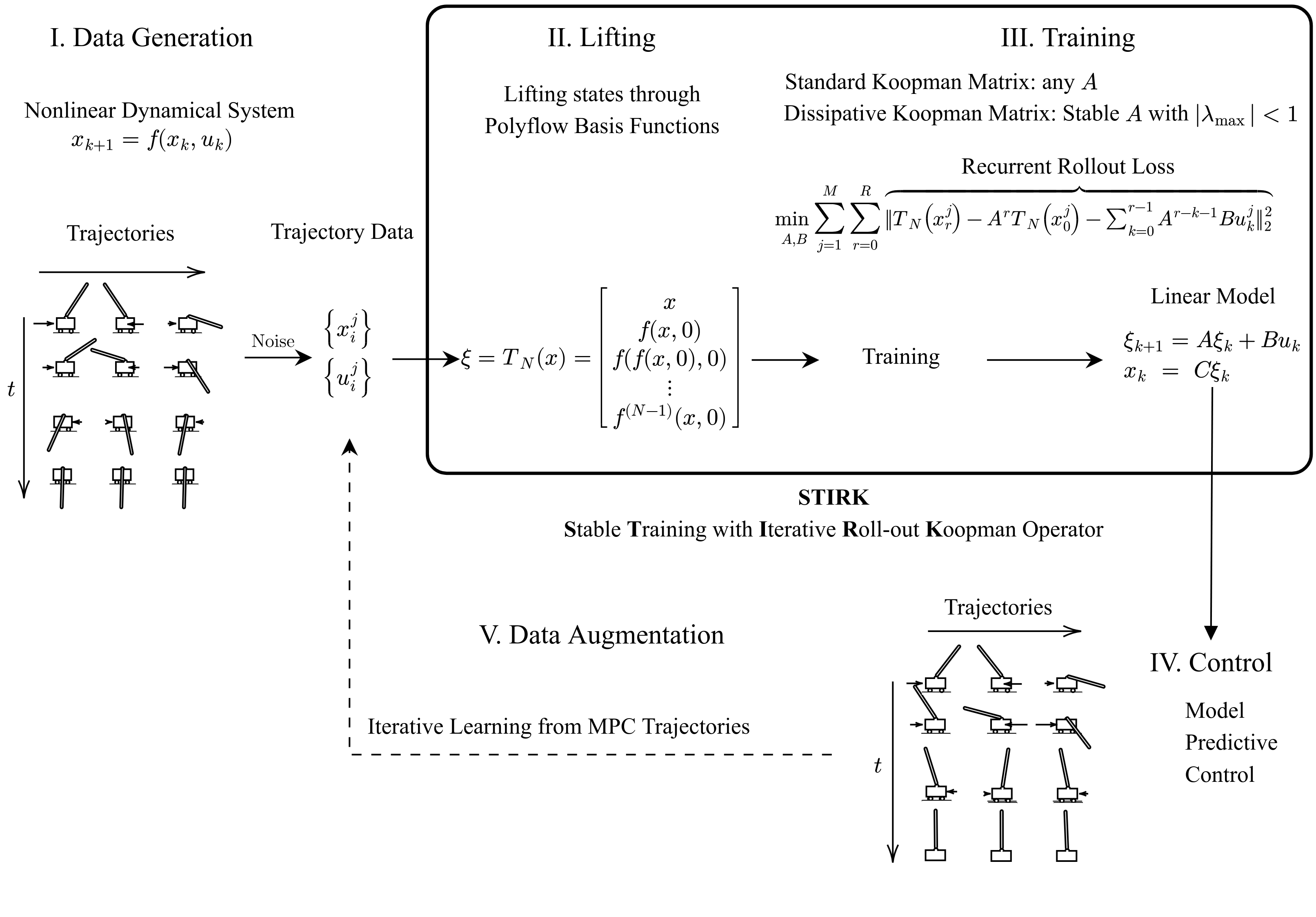
Models trained on trajectories that are generated by randomly sampling the phase space and control input could perform poorly when subjected to the optimal feedback control inputs. This is primarily because these trained models lack exposure to the desired scenarios during the training process, especially for relatively high-dimensional system. To address this issue, we propose a straightforward iterative data augmentation technique inspired by the work of Uchida and Duraisamy [45]. The idea is to iteratively collect response of the true system under control input synthesized with the previous data-driven model. Such response together with control input is used to augment the original dataset to further refine and improve the data-driven model. Our rationale is that such experience from the true system can be used to better explore the phase space of nonlinear system than merely ad-hoc random sampling the phase space, which is subject to the curse of dimensionality. Hence, our proposed framework is named as STIRK (Stable Training with Iterative Roll-out Koopman Operator). A summary of the proposed framework is illustrated in the figure 1.
III Numerical Experiments
In this section, we will evaluate our proposed framework against other popular frameworks by considering the following two tasks:
-
•
Prediction of the time evolution of Van der Pol oscillator given initial condition using the surrogate model learned with our framework;
-
•
Model predictive control of CartPole system given a surrogate model learned with our framework from noisy measurements.
III-A Prediction Performance
We compare the proposed framework with the following versions of DMD:
-
1.
DMD [46],
-
2.
eDMD [40]with Polyflow basis function and Radial Basis function,
-
3.
OptDMD [47] with Polyflow basis function, Radial Basis functions and Identity Observables,
-
4.
TLSDMD [48] with Polyflow basis function, Radial Basis functions and Identity Observables,
-
5.
FBDMD [49] with Polyflow basis function, Radial Basis functions and Identity Observables.
Van der Pol Oscillator.
We consider the autonomous Van der Pol Oscillator described by the equations:
| (18) | ||||
| (19) |
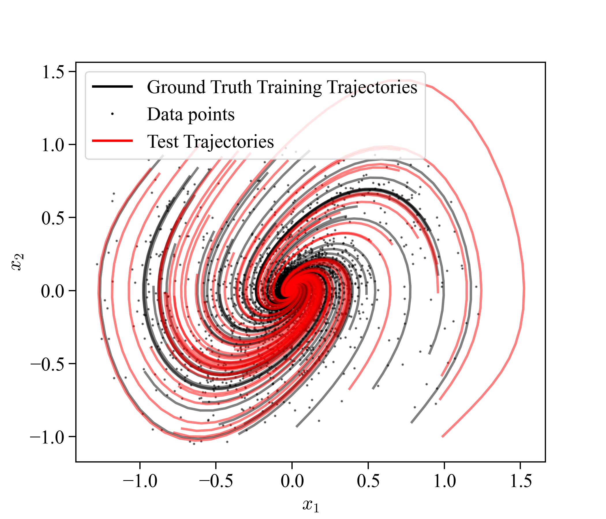
where is set to 1.0. The Van der Pol Oscillator is a nonlinear system characterized by a non-conservative force that can either dampen or amplify oscillations depending on the state. Since our framework relies on discrete-time dynamical system, the continuous-time version of Van der Pol system is discretized using a fourth-order Runge-Kutta method with a time step of 0.1. The training dataset is generated by running simulations for 100 steps, also with a time step of of 0.1. After the simulation, Gaussian noise is added to the states, with 10 noise levels logarithmically spaced from to . For models trained on a single trajectory, the initial condition is sampled from a normal distribution with a mean of and a standard deviation of . For models trained on multiple trajectories, 50 initial conditions are uniformly sampled from the range . To ensure robustness and generalizability, we created 10 sets of training data using different random seeds. Figure 2 illustrates one set of the training trajectories and test trajectories within the plane.
Prediction Performance Evaluation
To evaluate the prediction performance of the different algorithms, we use a normalized error metric that quantifies the discrepancy between the predicted trajectories and the ground truth trajectories. Let represent the true state of the system at time and represent the predicted state at time . The normalized prediction error over the trajectory is computed using the following formula:
| (20) |
where denotes the Frobenius norm, and and are the matrices containing the true and predicted states over all time steps , respectively,
| (21) |
Training
The Van der Pol system was initially trained using the Adam optimizer with a base learning rate of 0.01. A cyclic learning rate scheduler in triangular mode was employed, where the initial learning rate was halved each cycle. The maximum learning rate was set to 0.1, with each cycle stepping up for 500 epochs and stepping down for another 500 epochs. The Polyflow order was configured to 4. The training process spanned 15,000 epochs with a batch size of 1,000. The roll-out length was progressively increased, starting at 1 and doubling every 200 epochs, with a maximum roll-out length initially set to 90. In the final 1,000 epochs, the optimizer was switched to LBFGS with a learning rate of 0.01, applied on full batch data, to fine-tune the system.
Results for Single Trajectory
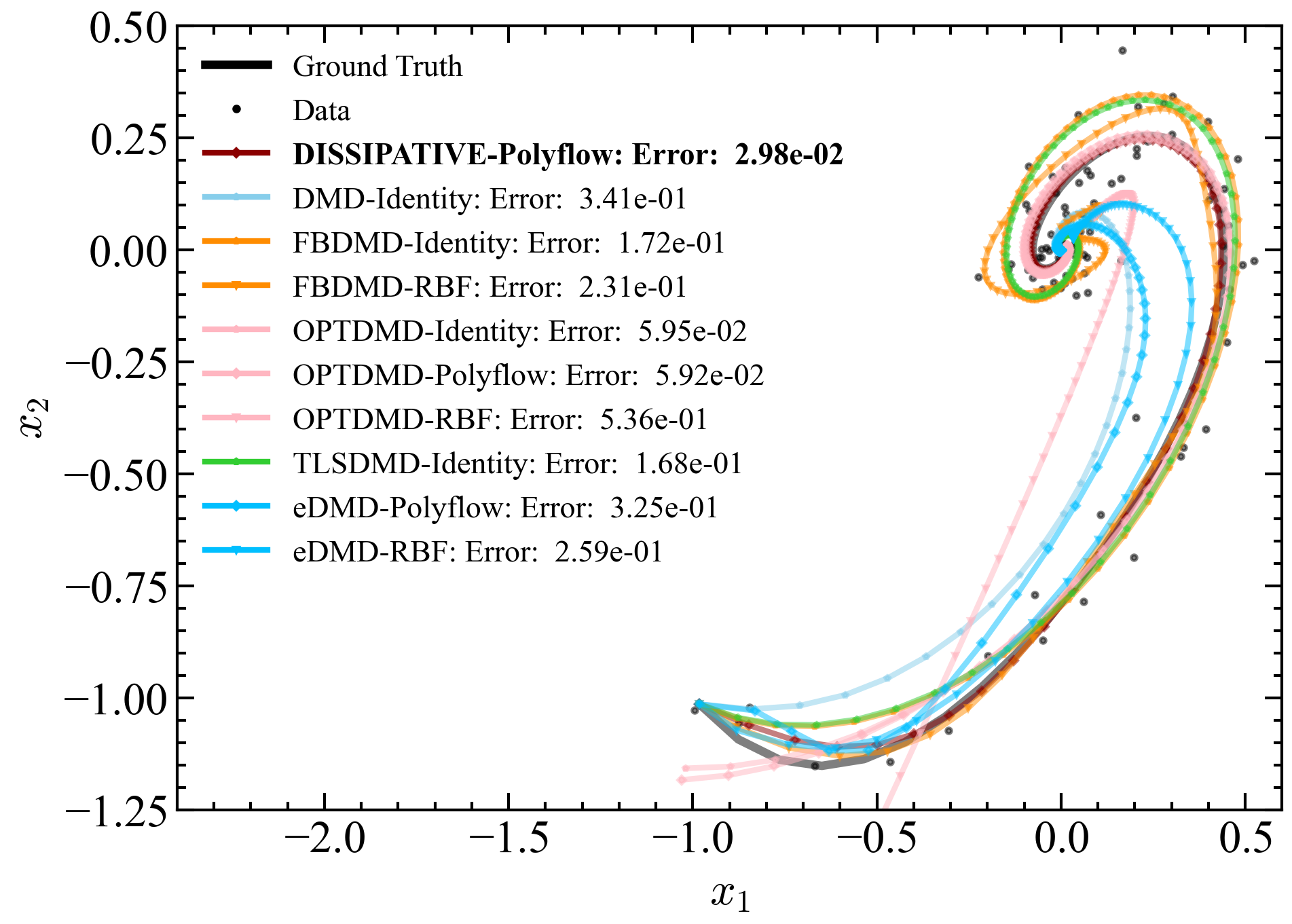
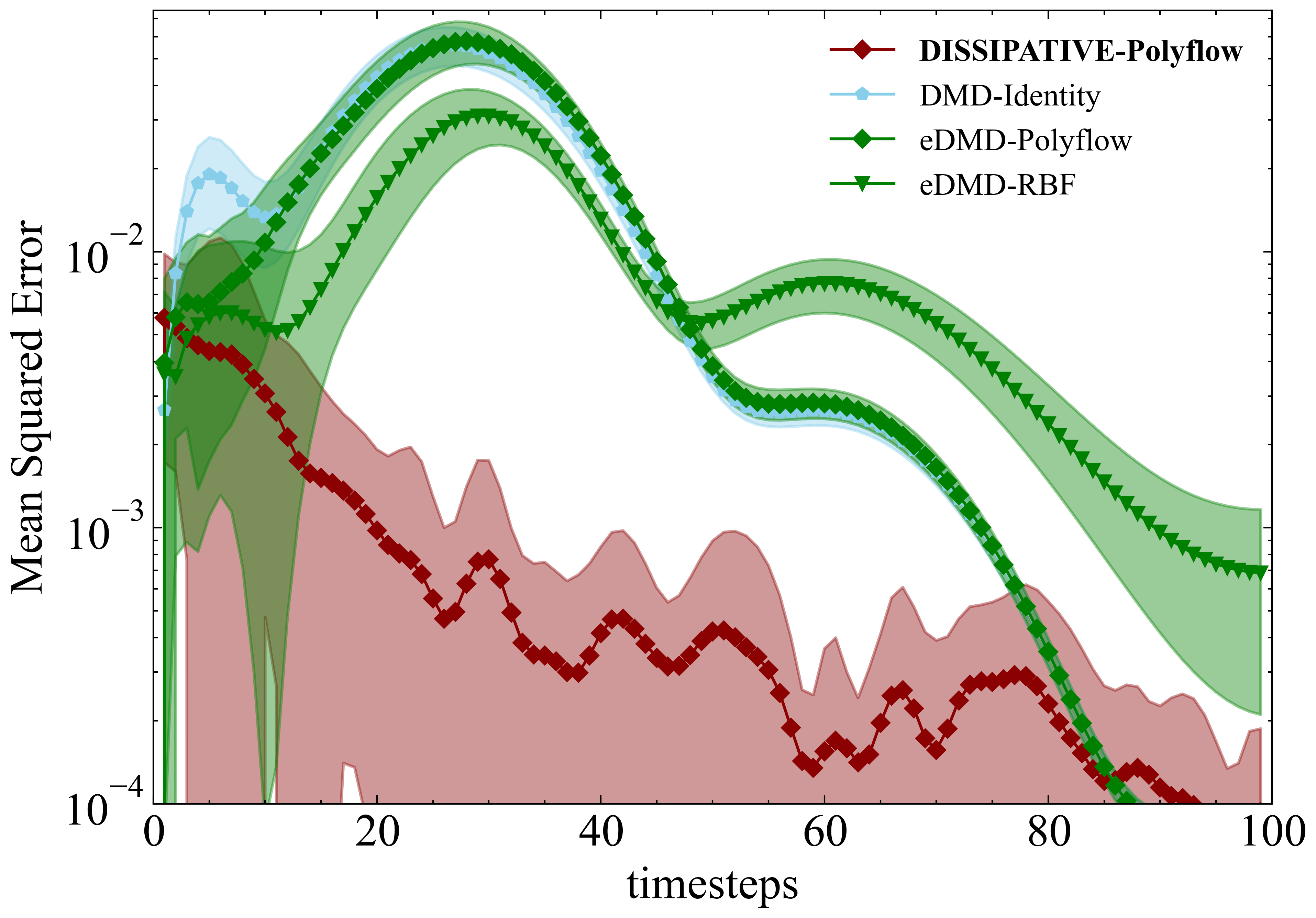
Figure 3a compares the reconstruction performance of various Dynamic Mode Decomposition (DMD)-based methods when trained on a single trajectory of the Van der Pol system at a noise level of 0.0599. The legend lists the normalized error for each method. The Dissipative Koopman model with Polyflow basis functions (DISSIPATIVE-Polyflow) achieved the lowest error of , indicating superior accuracy. OptDMD, using both identity and Polyflow basis functions, performed similarly well, closely approaching the performance of the Dissipative Koopman model. However, since OptDMD also optimizes the initial condition, it shows a deviation from the actual initial condition. Other methods exhibited higher errors, indicating less accurate reconstructions under the given noise conditions. Figure 3b presents the mean squared error (MSE) trajectory over 100 timesteps for the Van der Pol system at a noise level of 0.0599 for 10 different training sets. Each line represents the mean of the errors for a different DMD-based method, with shaded areas indicating the standard deviation of the error. The Dissipative Koopman model with Polyflow basis functions consistently maintains the lowest MSE across all timesteps, highlighting its robustness and accuracy under noisy conditions. The eDMD with Polyflow basis functions and the eDMD with RBF basis functions exhibit higher MSEs, particularly in the early timesteps, indicating less accurate predictions compared to the Dissipative model. The standard DMD with identity observables (DMD-Identity) also shows higher error compared to the Dissipative Koopman model but performs better than some of the other methods. The figures demonstrate that the Dissipative Koopman model with Polyflow basis functions outperforms other DMD-based methods in terms of prediction accuracy for the Van der Pol system under noisy conditions. This highlights the effectiveness of incorporating dissipative properties and structured observables in enhancing the robustness and accuracy of the model.
Results for Multiple Trajectories
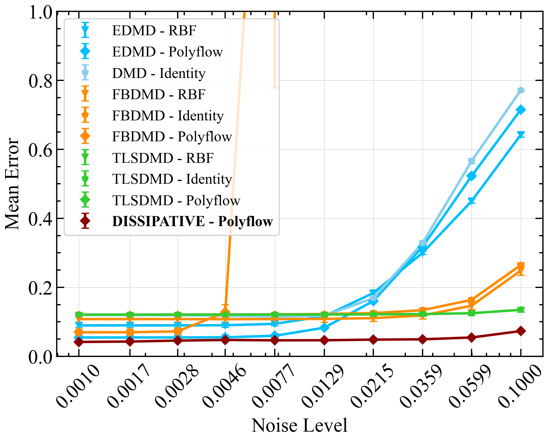
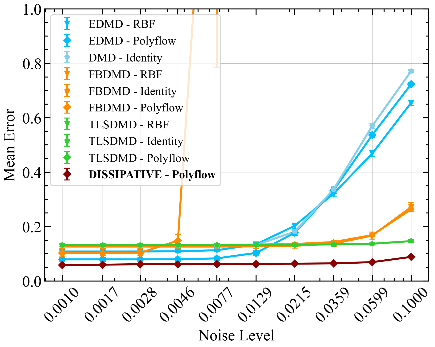
Figure 4 compares the prediction errors for multiple trajectories of the Van der Pol (VDP) system across different noise levels. Panel (a) shows the training error, while panel (b) shows the test error. The Dissipative Koopman model with Polyflow basis functions consistently shows lower errors across various noise levels, demonstrating its robustness and accuracy in handling multiple trajectories.
| Strategy | DMD | FBDMD | TLSDMD | eDMD | DISSIPATIVE (Ours) | ||||||
| Lifting Function | Identity | Identity | Polyflow | RBF | Identity | Polyflow | RBF | Polyflow | RBF | Polyflow | |
| Error Type | Noise | ||||||||||
| Mean Normalized Training Error | 0.0010 | 0.1198 | 0.1211 | 0.0697 | 0.1079 | 0.1210 | NaN | NaN | 0.0547 | 0.0898 | 0.0417 |
| 0.0599 | 0.5660 | 0.1638 | NaN | 0.1468 | 0.1249 | NaN | NaN | 0.5225 | 0.4500 | 0.0547 | |
| 0.1000 | 0.7711 | 0.2647 | NaN | 0.2486 | 0.1348 | NaN | NaN | 0.7149 | 0.6420 | 0.0733 | |
| Mean Normalized Test Error | 0.0010 | 0.1315 | 0.1326 | 0.1028 | 0.1268 | 0.1325 | NaN | NaN | 0.0796 | 0.1085 | 0.0590 |
| 0.0599 | 0.5704 | 0.1691 | NaN | 0.1671 | 0.1370 | NaN | NaN | 0.5370 | 0.4688 | 0.0694 | |
| 0.1000 | 0.7715 | 0.2634 | NaN | 0.2718 | 0.1468 | NaN | NaN | 0.7235 | 0.6552 | 0.0888 | |
III-B Control Performance
CartPole System
Let us consider the CartPole System,
| (22) | ||||
| (23) | ||||
| (24) | ||||
| (25) |
The CartPole system consists of a cart that moves along a track, balancing a pole attached to it via a pivot. The dynamics of the system are described by the equations above, where represents the position of the cart, represents the angle of the pole, represents the velocity of the cart, represents the angular velocity of the pole, and is the control input force applied to the cart. The parameters of the system include the mass of the cart (), the mass of the pole (), the length of the pole (), and the acceleration due to gravity (). For our framework, the continuous-time CartPole system is discretized using a fourth-order Runge-Kutta method with a time step of 0.05. The training dataset is generated by running simulations for 200 steps and contains 50 different trajectories. After the simulation, Gaussian noise is added to the states with noise level of 0.1. The initial conditions for the CartPole system are randomly sampled with the position () from , the angle () from , the velocity () from , and the angular velocity () from . Control inputs are generated using exponentially decaying sine waves of randomly sampled frequencies, amplitudes and phase angles.
Training
The CartPole system was trained using the Adam optimizer with a learning rate of 0.001. The Polyflow order was set to 4. The training dataset consisted of 45 trajectories, while 5 trajectories were reserved for validation. The training process spanned 5,000 epochs with a batch size of 2,000. The maximum roll-out length was set to 32 and the roll-out length was increased every 300 epochs by a factor of 2.
MPC Configuration
The trained Koopman model is used as a surrogate model for model predictive control, following the approach in [18]. The prediction horizon, , is set to 20 steps. Control input constraints are defined as and , with no constraints on the system states. For the cost function described in eq. 17, and are set to ones on the first diagonal elements, with zeros elsewhere. The parameter is set to 0.
Results
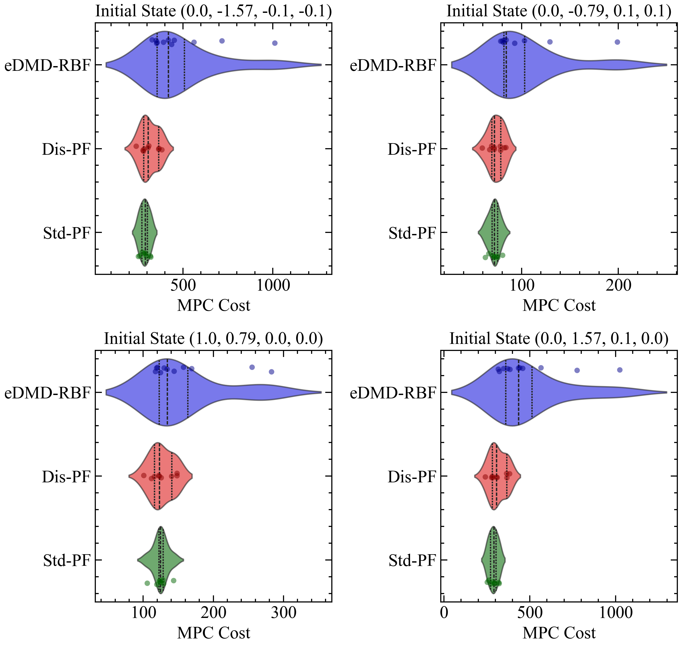
Figure 5 compares the Model Predictive Control (MPC) costs for the CartPole system using three different models under a noise level of 0.100. The models compared are EDMD with RBF basis functions (eDMD-RBF), the Dissipative Koopman model with Polyflow basis functions (Dis-PF), and the Standard Koopman model with Polyflow basis functions (Std-PF). The violin plots illustrate the distribution of MPC costs across various initial states. The results indicate that both the Dissipative Koopman model with Polyflow basis functions (Dis-PF) and the Standard Koopman model with Polyflow basis functions (Std-PF) achieve relatively similar MPC costs. Both models show stable control performance across different initial states, demonstrating robustness in control. In contrast, the EDMD with RBF basis functions (eDMD-RBF) exhibits higher variability in MPC costs and generally incurs higher average MPC costs compared to the Dissipative and Standard Koopman models. This suggests that while the EDMD-RBF model provides some level of stability, it does so at the expense of higher control costs and less consistency. Overall, the comparison reveals that both the Dissipative and Standard Koopman models with Polyflow basis functions offer superior and more stable control performance compared to the EDMD-RBF model under the noise level of 0.1. This highlights the effectiveness of the Polyflow basis functions in achieving robust control in MPC applications.
IV Iterative Data Augmentation
To explore the phase space of a nonlinear system more effectively, we introduce an iterative data augmentation technique. Instead of relying solely on ad-hoc random sampling, we augment the training data with failure trajectories from closed-loop control and then retrain the Koopman operator. This approach addresses challenges highlighted by [50], where the authors emphasize the need to identify inputs that closely approximate the final closed-loop input and to use randomized signals that resemble it. However, finding suitable randomized control signals can be challenging and may not be adequate for control tasks. Therefore, we propose a rather automated approach: augmenting the training data with control signals from previous failed control tasks in a closed-loop setting. This approach involves collecting the system’s response to control inputs from data-driven based model predictive controller. The responses, along with the corresponding control inputs, are used to enhance the original dataset, enabling further refinement and improvement of the model.
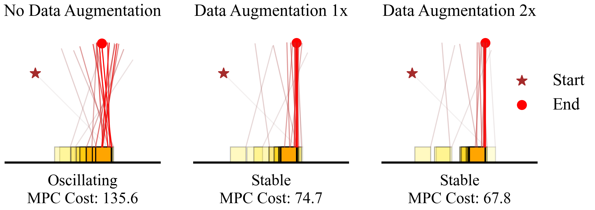
Figure 6 visualizes the trajectory of the CartPole system across three different scenarios: no data augmentation, one-time data augmentation, and twice data augmentation. In the first scenario, where no data augmentation was applied, the Koopman model fails to stabilize the CartPole after 200 steps. However, when the failed trajectory, along with other failed trajectories from different initial conditions, is added to the training data, the Koopman model demonstrates significantly improved control outcomes. The performance notably improves with data augmentation, transitioning from oscillating to stable trajectories. This enhancement is also reflected in the reduction of the Model Predictive Control (MPC) cost, with costs decreasing from 135.6 (no augmentation) to 74.7 (one-time augmentation) and 67.8 (twice augmentation).
Figure 7 presents violin plots illustrating the distribution of Model Predictive Control (MPC) costs for the CartPole system across two different tasks—seen and unseen—and iterative models under a noise level of 0.1. The “seen” task refers to scenarios where input bounds are set between , while the “unseen” task refers to tighter input bounds of . Data augmentation was performed using closed loop trajectories from the seen task. It is important to note that classical iterative learning [51] cannot easily generalize to a different task. The violin plots display MPC costs for four different initial states and two levels of data augmentation, comparing the costs for both control tasks. Each subplot emphasizes the performance gains achieved through iterative learning. The results indicate that both seen and unseen control tasks benefit significantly from iterative learning, with successive iterations leading to lower and more stable MPC costs. This demonstrates the effectiveness of iterative learning in enhancing the overall performance of the system.
V Ablation Studies
In this section, we will analyze the individual effect of the following components on the overall model performance with training data at different noise levels for Van der Pol Oscillator system:
-
•
Stabilized formulation of Koopman operator in Section II-F,
-
•
Learning rate scheduler,
-
•
Optimizer switching,
-
•
Progressive roll-out.
V-A Dissipative Koopman Model versus Standard Koopman Model
Figure 9a compares the performance of the Dissipative Koopman Model and the Standard Koopman Model across different noise levels. The Dissipative Koopman Model consistently shows lower mean errors and mean test errors, underscoring its superior prediction accuracy and robustness. However, the training time for the Dissipative Koopman Model is considerably longer than that of the Standard Koopman Model, due to the increased number of learning parameters and the computationally intensive operations, such as matrix exponentiation and pseudo-inverse computation. Despite its relatively short training time, a significant drawback of the Standard Koopman Model is its sensitivity to the initial conditions of the Koopman matrix. If these initial conditions are not carefully tuned, the model can produce unstable eigenvalues, leading to poor performance. Figure 8 illustrates this issue by showing the discrete-time eigenvalues of the standard and dissipative Koopman operators for the Van der Pol Oscillator System at a noise level of 0.0599, using a different weight initialization than in previous cases. For fair comparison, both standard and dissipative Koopman models are initialized with stable Koopman matrices. However, after 1,000 training epochs, some of the discrete-time eigenvalues in the Standard Koopman matrix move outside the unit circle, leading to a loss of stability while dissipative Koopman model never loses stability during training.
V-B Learning Rate Scheduler
Figure 9b compares the performance of the model using constant learning rate (LR) scheduling and cyclic learning rate scheduling under different noise levels. For low noise, the cyclic learning rate scheduling achieves a 20% reduction in training error and a 16.67% reduction in test error, with a 9.09% reduction in time taken compared to the constant learning rate. In medium noise scenarios, the cyclic learning rate scheduling shows a 16.67% improvement in training error, 14.29% in test error, and an 8.70% improvement in time taken. However, at high noise levels, cyclic learning rate scheduling underperforms compared to the constant learning rate, with higher training and test errors, as well as slightly longer training times. These results indicate that while the cyclic learning rate scheduler is beneficial at low and medium noise levels, it is less effective in high-noise environments.
V-C Optimizer Switching
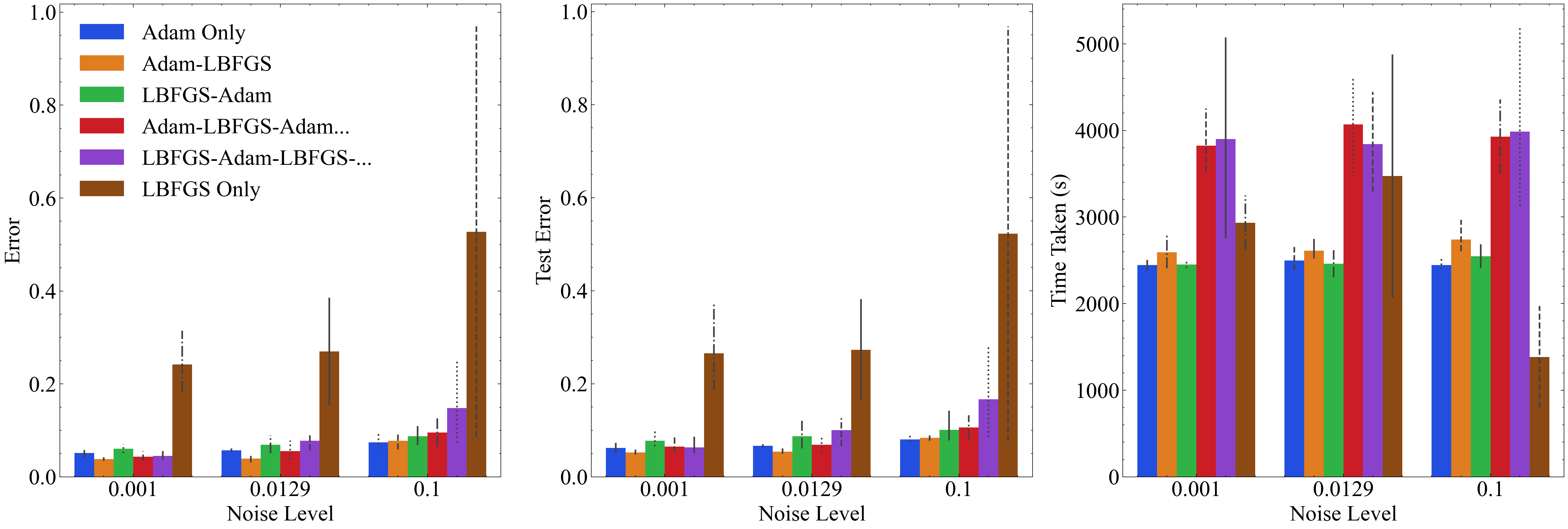
Figure 9c examines the effect of switching optimizers on the model’s performance. Different combinations of Adam and LBFGS optimizers were used, and their impact on mean errors, mean test errors, and training times was analyzed. Switching from the Adam optimizer to LBFGS after 4000 epochs in a 5000-epoch training cycle resulted in about a 25% error reduction compared to the Adam-only optimizer at low and medium noise levels, demonstrating the efficacy of LBFGS during fine-tuning. However, this advantage diminished at higher noise levels, where the differences between the optimizers became less pronounced. In experiments where optimizers were switched periodically every 500 epochs, results varied, but overall, periodic switching helped minimize the error in certain cases, though it did not consistently outperform the Adam-LBFGS approach. Notably, using only LBFGS led to significantly higher errors, suggesting that while LBFGS is beneficial for fine-tuning, it tends to settle in local minima and does not further improve the error.
V-D Progressive roll-out length versus Constant roll-out length
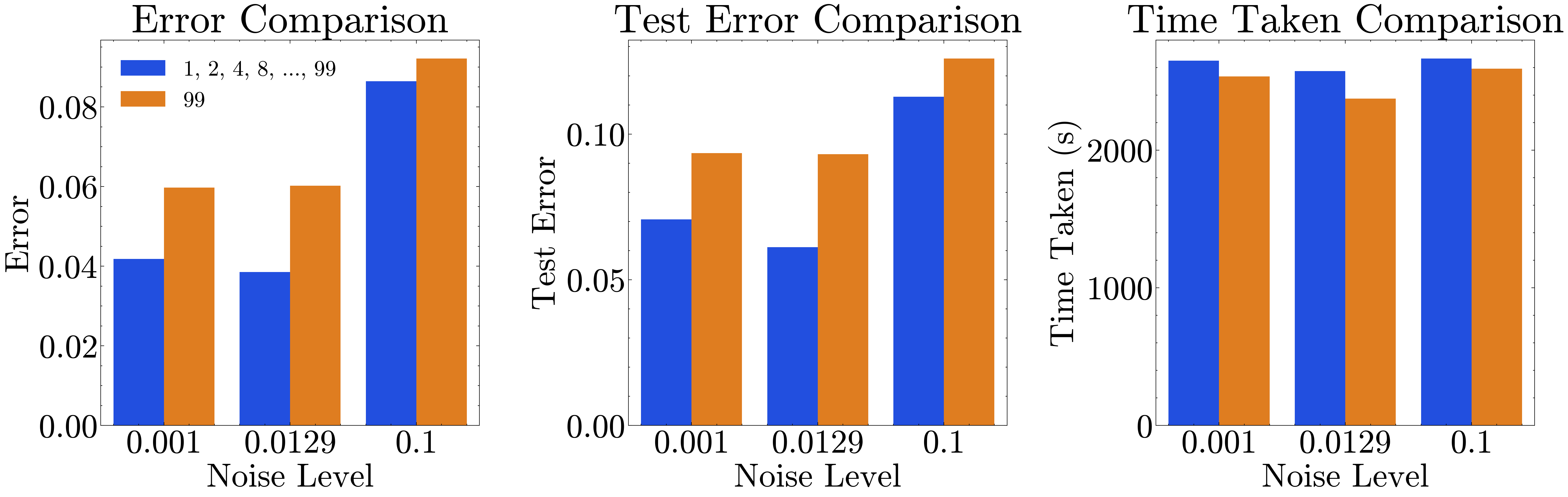
Figure 9d compares the performance of the model using progressive roll-out length scheduling and constant roll-out length scheduling under different noise levels. Progressive roll-out scheduling shows a 20% improvement in mean training errors and a 16.67% improvement in mean test errors compared to the constant roll-out length, indicating better learning and generalization. Although the time taken for training with progressive roll-out scheduling is 6.94% lower, the overall training duration remains slightly higher due to the incremental increase in roll-out length. These results highlight the effectiveness of progressive roll-out scheduling in enhancing model performance.
V-E Overall Impact of Optimized Training Strategy
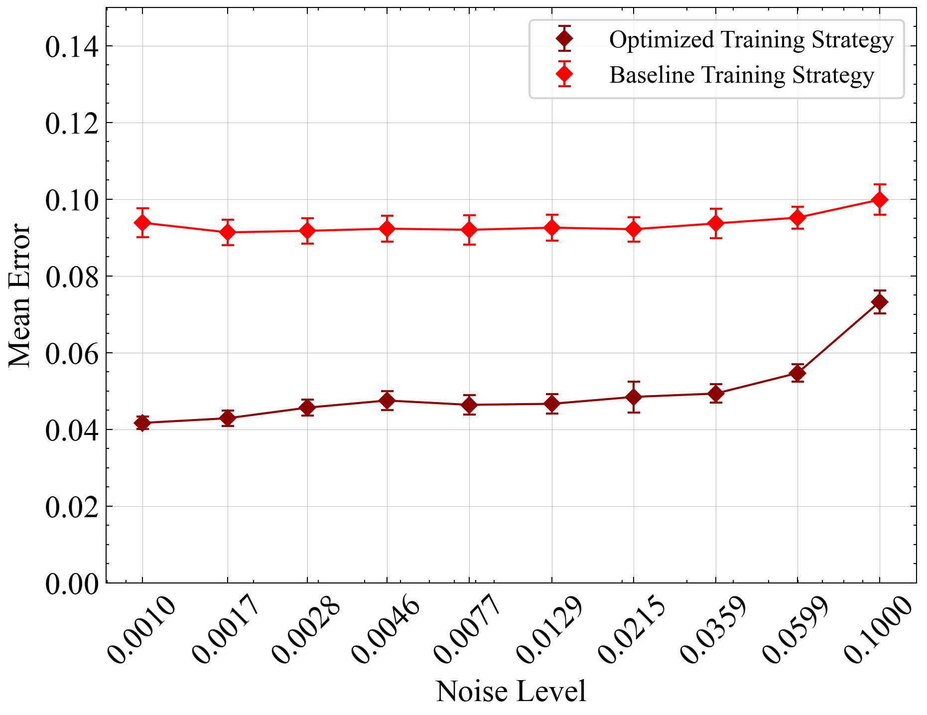
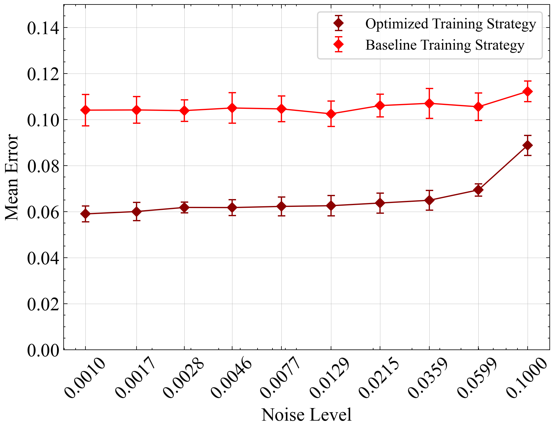
Finally, we compare the overall performance of our optimized configuration with the baseline configuration, as shown in 10 and 11. 10 shows the prediction performance comparison for Van der Pol system and 11 shows the Model Predictive Costs comparison for Cartpole system.
For the Van der Pol system 10, the baseline setup utilized a standard Koopman operator with a fixed maximum rollout length of 99, without any learning rate scheduler, and maintained a constant learning rate of 0.01. In contrast, our optimized configuration employed a dissipative Koopman operator alongside a progressive rollout strategy, starting with a rollout length of 1 and geometrically increasing by a factor of 2 every 200 epochs until reaching the maximum rollout length. Additionally, we implemented a cyclic learning rate scheduler in triangular mode, with the maximum learning rate set to 0.1, halving every 500 epochs, and a base learning rate of 0.01. Both configurations used the Adam optimizer. Overall, the optimized configuration resulted in a 39% improvement in training error and a 37.6% improvement in testing error compared to the baseline. This significant reduction in error highlights how the combined components of the optimized configuration effectively enhance the model’s performance.
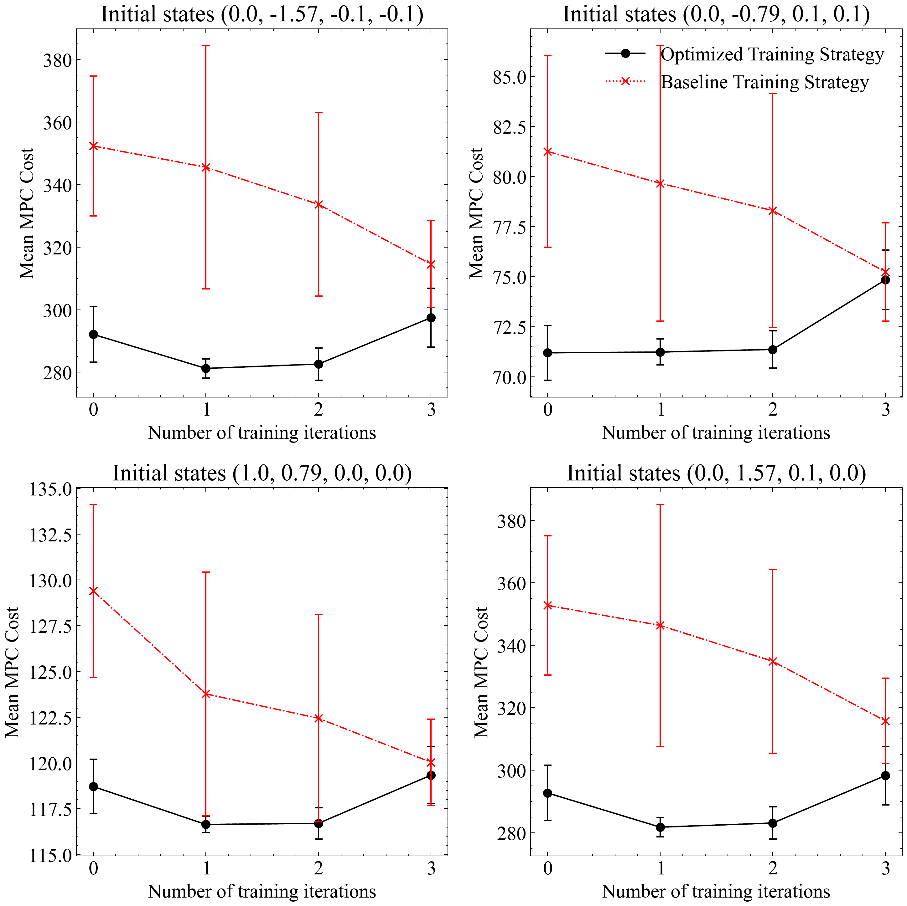
In the case of the Cartpole system (11, the baseline strategy used the Adam optimizer with a constant rollout length of 16 and a constant learning rate. The standard Koopman operator was utilized throughout the training. Conversely, the optimized strategy employed the Adam optimizer for the initial 1500 epochs, followed by fine-tuning using the LBFGS optimizer. The rollout length was progressively increased from 1 to 16, a cyclic learning rate was implemented, and a dissipative Koopman operator was used. The optimized training strategy outperforms the baseline training strategy across different initial conditions over multiple iterative training data augmentations.
VI Conclusions
In this work, we proposed a novel data-driven learning framework for the Koopman operator of nonlinear dynamical systems. Unlike existing frameworks that rely on ad-hoc observables or complex neural networks to approximate the Koopman invariant subspace, our approach utilizes observables generated by the system dynamics through a Hankel matrix. This data-driven time-delay embedding significantly enhances the performance and robustness of the resulting models compared to ad-hoc choices. To ensure noise robustness and long-term stability of the lifted system, we designed a stable parameterization of the Koopman operator and employed a roll-out recurrent loss. Our stabilized parameterization guarantees a stable system, which is equally accurate or, in some cases, even more accurate than the standard Koopman operator. Additionally, we addressed the curse of dimensionality in sampling from high-dimensional phase space by iteratively augmenting data from closed-loop trajectories. This approach not only improved performance in seen closed-loop scenarios but also enhanced the model’s ability to handle unseen control objectives effectively. We conducted an ablation study to demonstrate the effectiveness of several key components: switching to the LBFGS optimizer for fine-tuning, employing cyclic learning rate scheduling, utilizing progressive roll-out lengths for enhanced training outcomes, and incorporating a stabilized Koopman operator to ensure guaranteed system stability. Our numerical results on the Van der Pol Oscillator and the CartPole system demonstrated the superior performance of the proposed framework in prediction and model predictive control (MPC) of nonlinear systems, compared to other popular DMD-based methods. In summary, our framework offers a noise-robust approach for learning stable Koopman operators, providing a solid foundation for future research (e.g., Koopman for reinforcement learning [11]) and applications in nonlinear dynamical system control.
Acknowledgement
The authors are thankful for the provision of computational resources from the Center for Computational Innovations (CCI) at Rensselaer Polytechnic Institute (RPI) during the early stages of this research. Numerical experiments are performed using the computational resources granted by NSF-ACCESS for the project PHY240112 and that of the National Energy Research Scientific Computing Center, a DOE Office of Science User Facility using NERSC award NERSC DDR-ERCAP0030714.
References
- [1] S. L. Brunton, M. Budišić, E. Kaiser, and J. N. Kutz, “Modern koopman theory for dynamical systems,” arXiv preprint arXiv:2102.12086, 2021.
- [2] H. J. Van Waarde, J. Eising, H. L. Trentelman, and M. K. Camlibel, “Data informativity: A new perspective on data-driven analysis and control,” IEEE Transactions on Automatic Control, vol. 65, no. 11, pp. 4753–4768, 2020.
- [3] B. O. Koopman, “Hamiltonian systems and transformation in hilbert space,” Proceedings of the National Academy of Sciences, vol. 17, no. 5, pp. 315–318, 1931.
- [4] I. Mezić, “Spectral properties of dynamical systems, model reduction and decompositions,” Nonlinear Dynamics, vol. 41, no. 1-3, pp. 309–325, 2005.
- [5] M. Budišić, R. Mohr, and I. Mezić, “Applied koopmanism,” Chaos: An Interdisciplinary Journal of Nonlinear Science, vol. 22, no. 4, p. 047510, 2012.
- [6] I. Mezić, “Analysis of fluid flows via spectral properties of the koopman operator,” Annual Review of Fluid Mechanics, vol. 45, pp. 357–378, 2013.
- [7] S. E. Otto and C. W. Rowley, “Koopman operators for estimation and control of dynamical systems,” Annual Review of Control, Robotics, and Autonomous Systems, vol. 4, pp. 59–87, 2021.
- [8] P. Bevanda, S. Sosnowski, and S. Hirche, “Koopman operator dynamical models: Learning, analysis and control,” Annual Reviews in Control, vol. 52, pp. 197–212, 2021.
- [9] I. Mezic, “Operator is the model,” arXiv preprint arXiv:2310.18516, 2023.
- [10] I. Mezić, Z. Drmač, N. Črnjarić, S. Maćešić, M. Fonoberova, R. Mohr, A. M. Avila, I. Manojlović, and A. Andrejčuk, “A koopman operator-based prediction algorithm and its application to covid-19 pandemic and influenza cases,” Scientific reports, vol. 14, no. 1, p. 5788, 2024.
- [11] P. Rozwood, E. Mehrez, L. Paehler, W. Sun, and S. L. Brunton, “Koopman-assisted reinforcement learning,” arXiv preprint arXiv:2403.02290, 2024.
- [12] D. Bruder, X. Fu, R. B. Gillespie, C. D. Remy, and R. Vasudevan, “Koopman-based control of a soft continuum manipulator under variable loading conditions,” IEEE robotics and automation letters, vol. 6, no. 4, pp. 6852–6859, 2021.
- [13] J. Harrison and E. Yeung, “Stability analysis of parameter varying genetic toggle switches using koopman operators,” Mathematics, vol. 9, no. 23, p. 3133, 2021.
- [14] C. R. Constante-Amores, A. J. Fox, C. E. P. De Jesús, and M. D. Graham, “Data-driven koopman operator predictions of turbulent dynamics in models of shear flows,” arXiv preprint arXiv:2407.16542, 2024.
- [15] M. Korda and I. Mezić, “Linear predictors for nonlinear dynamical systems: Koopman operator meets model predictive control,” arXiv preprint arXiv:1611.03537, 2016.
- [16] E. Kaiser, J. N. Kutz, and S. L. Brunton, “Data-driven discovery of koopman eigenfunctions for control,” Machine Learning: Science and Technology, vol. 2, no. 3, p. 035023, 2021.
- [17] A. Surana and A. Banaszuk, “Linear observer synthesis for nonlinear systems using koopman operator framework,” IFAC-PapersOnLine, vol. 49, no. 18, pp. 716–723, 2016.
- [18] M. Korda and I. Mezić, “Linear predictors for nonlinear dynamical systems: Koopman operator meets model predictive control,” Automatica, vol. 93, pp. 149–160, 2018.
- [19] S. Peitz, S. E. Otto, and C. W. Rowley, “Data-driven model predictive control using interpolated koopman generators,” SIAM Journal on Applied Dynamical Systems, vol. 19, no. 3, pp. 2162–2193, 2020.
- [20] S. Qian and C.-A. Chou, “A koopman-operator-theoretical approach for anomaly recognition and detection of multi-variate eeg system,” Biomedical Signal Processing and Control, vol. 69, p. 102911, 2021.
- [21] M. Bakhtiaridoust, M. Yadegar, and F. Jahangiri, “Koopman fault-tolerant model predictive control,” IET Control Theory & Applications, vol. 18, no. 7, pp. 939–950, 2024.
- [22] Q. Li, F. Dietrich, E. M. Bollt, and I. G. Kevrekidis, “Extended dynamic mode decomposition with dictionary learning: A data-driven adaptive spectral decomposition of the koopman operator,” Chaos: An Interdisciplinary Journal of Nonlinear Science, vol. 27, no. 10, p. 103111, 2017.
- [23] S. L. Brunton, B. W. Brunton, J. L. Proctor, and J. N. Kutz, “Koopman invariant subspaces and finite linear representations of nonlinear dynamical systems for control,” PloS one, vol. 11, no. 2, p. e0150171, 2016.
- [24] S. Otto, S. Peitz, and C. Rowley, “Learning bilinear models of actuated koopman generators from partially observed trajectories,” SIAM Journal on Applied Dynamical Systems, vol. 23, no. 1, pp. 885–923, 2024.
- [25] R. M. Jungers and P. Tabuada, “Non-local linearization of nonlinear differential equations via polyflows,” in 2019 American Control Conference (ACC). IEEE, 2019, pp. 1–6.
- [26] G. Mamakoukas, M. L. Castano, X. Tan, and T. D. Murphey, “Derivative-based koopman operators for real-time control of robotic systems,” IEEE Transactions on Robotics, vol. 37, no. 6, pp. 2173–2192, 2021.
- [27] I. Mezić, “On numerical approximations of the koopman operator,” Mathematics, vol. 10, no. 7, p. 1180, 2022.
- [28] Z. Wang and R. M. Jungers, “Immersion-based model predictive control of constrained nonlinear systems: Polyflow approximation,” in 2021 European Control Conference (ECC). IEEE, 2021, pp. 1099–1104.
- [29] Z. Wu, S. L. Brunton, and S. Revzen, “Challenges in dynamic mode decomposition,” Journal of the Royal Society Interface, vol. 18, no. 185, p. 20210686, 2021.
- [30] S. E. Otto and C. W. Rowley, “Linearly recurrent autoencoder networks for learning dynamics,” SIAM Journal on Applied Dynamical Systems, vol. 18, no. 1, pp. 558–593, 2019.
- [31] B. Lusch, J. N. Kutz, and S. L. Brunton, “Deep learning for universal linear embeddings of nonlinear dynamics,” Nature Communications, vol. 9, no. 1, p. 4950, 2018.
- [32] S. Pan and K. Duraisamy, “Physics-informed probabilistic learning of linear embeddings of nonlinear dynamics with guaranteed stability,” SIAM Journal on Applied Dynamical Systems, vol. 19, no. 1, pp. 480–509, 2020.
- [33] W. I. T. Uy, D. Hartmann, and B. Peherstorfer, “Operator inference with roll outs for learning reduced models from scarce and low-quality data,” Computers & Mathematics with Applications, vol. 145, pp. 224–239, 2023.
- [34] P. Bevanda, M. Beier, S. Kerz, A. Lederer, S. Sosnowski, and S. Hirche, “Diffeomorphically learning stable koopman operators,” IEEE Control Systems Letters, vol. 6, pp. 3427–3432, 2022.
- [35] M. J. Colbrook, I. Mezić, and A. Stepanenko, “Limits and powers of koopman learning,” arXiv preprint arXiv:2407.06312, 2024.
- [36] D. Bruder, X. Fu, and R. Vasudevan, “Advantages of bilinear koopman realizations for the modeling and control of systems with unknown dynamics,” IEEE Robotics and Automation Letters, vol. 6, no. 3, pp. 4369–4376, 2021.
- [37] S. Yu, C. Shen, and T. Ersal, “Autonomous driving using linear model predictive control with a koopman operator based bilinear vehicle model,” IFAC-PapersOnLine, vol. 55, no. 24, pp. 254–259, 2022.
- [38] D. Goswami and D. A. Paley, “Bilinearization, reachability, and optimal control of control-affine nonlinear systems: A koopman spectral approach,” IEEE Transactions on Automatic Control, vol. 67, no. 6, pp. 2715–2728, 2021.
- [39] C. Folkestad, S. X. Wei, and J. W. Burdick, “Koopnet: Joint learning of koopman bilinear models and function dictionaries with application to quadrotor trajectory tracking,” in 2022 International Conference on Robotics and Automation (ICRA). IEEE, 2022, pp. 1344–1350.
- [40] M. O. Williams, I. G. Kevrekidis, and C. W. Rowley, “A data–driven approximation of the koopman operator: Extending dynamic mode decomposition,” Journal of Nonlinear Science, vol. 25, no. 6, pp. 1307–1346, 2015.
- [41] S. L. Brunton, B. W. Brunton, J. L. Proctor, E. Kaiser, and J. N. Kutz, “Chaos as an intermittently forced linear system,” Nature communications, vol. 8, no. 1, p. 19, 2017.
- [42] S. L. Brunton, J. L. Proctor, and J. N. Kutz, “Discovering governing equations from data by sparse identification of nonlinear dynamical systems,” Proceedings of the National Academy of Sciences, p. 201517384, 2016.
- [43] R. T. Chen, Y. Rubanova, J. Bettencourt, and D. K. Duvenaud, “Neural ordinary differential equations,” Advances in neural information processing systems, vol. 31, 2018.
- [44] Y. Bengio, J. Louradour, R. Collobert, and J. Weston, “Curriculum learning,” in Proceedings of the 26th annual international conference on machine learning, 2009, pp. 41–48.
- [45] D. Uchida and K. Duraisamy, “Control-aware learning of koopman embedding models,” in 2023 American Control Conference (ACC). IEEE, 2023, pp. 941–948.
- [46] J. H. Tu, C. W. Rowley, D. M. Luchtenburg, S. L. Brunton, and J. N. Kutz, “On dynamic mode decomposition: theory and applications,” arXiv preprint arXiv:1312.0041, 2013.
- [47] T. Askham and J. N. Kutz, “Variable projection methods for an optimized dynamic mode decomposition,” SIAM Journal on Applied Dynamical Systems, vol. 17, no. 1, pp. 380–416, 2018.
- [48] Y. Ohmichi, Y. Sugioka, and K. Nakakita, “Stable dynamic mode decomposition algorithm for noisy pressure-sensitive-paint measurement data,” AIAA Journal, vol. 60, no. 3, pp. 1965–1970, 2022.
- [49] S. T. Dawson, M. S. Hemati, M. O. Williams, and C. W. Rowley, “Characterizing and correcting for the effect of sensor noise in the dynamic mode decomposition,” Experiments in Fluids, vol. 57, no. 3, p. 42, 2016.
- [50] L. Do, A. Uchytil, and Z. Hurák, “Practical guidelines for data-driven identification of lifted linear predictors for control,” arXiv preprint arXiv:2408.01116, 2024.
- [51] S. Mishra, U. Topcu, and M. Tomizuka, “Optimization-based constrained iterative learning control,” IEEE Transactions on Control Systems Technology, vol. 19, no. 6, pp. 1613–1621, 2010.
VII Biography Section
| Shahriar Akbar Sakib is currently a second-year Ph.D. student in Mechanical Engineering at Rensselaer Polytechnic Institute in Troy, NY. He earned his B.Sc. in Mechanical Engineering from the Bangladesh University of Engineering and Technology in 2021. His research focuses on data-driven modeling and control of complex nonlinear dynamical systems, as well as machine learning. |
| Shaowu Pan received the B.S. degree in Aerospace Engineering and Applied Mathematics from Beihang University, China, in 2013. He earned the M.S. and Ph.D. degrees in Aerospace Engineering and Scientific Computing from the University of Michigan, Ann Arbor, in April 2021. Following this, he was a Postdoctoral Scholar at the AI Institute in Dynamic Systems, University of Washington, Seattle. His research interests include data-driven modeling and control of complex nonlinear systems, scientific machine learning, and dynamical systems. |