Learning Many-to-Many Mapping for Unpaired Real-World Image Super-resolution and Downscaling

Normalizing flow [39], as a type of latent variable generative model, is to explicitly estimate the probability distribution of the input data. Compared to GAN [20] and variational autoencoder (VAE) [50], normalizing flow features exact likelihood estimation, efficient sample generation, and stable training. Typically, flow-based models try to learn a bijective mapping between the data space and the latent space. Specifically, let $(\mathbf{x}\in\mathbb{R}^{d})\sim p(\mathbf{X})$ be a $d$ dimensional random variable with complex marginal distribution, the main idea of flow-based models is the employment of a learned invertible function $f_{\theta}(\cdot)$ transforming $\mathbf{x}$ to $(\mathbf{z}\in\mathbb{R}^{d})\sim p(\mathbf{Z})$ with simple and tractable distribution (e.g.  Gaussian distribution). Since $f_{\theta}(\cdot)$ is invertible, it implies a one-to-one mapping between the input and output. Thus, the data can be losslessly restored from the latent variable as $\mathbf{x}=f_{\theta}^{-1}(\mathbf{z})$. Making the use of change-of-variables rule, the log-likelihood the of data $\mathbf{x}$ can be written as:

where $\phi$ is the parameter of the base distribution, e.g.  for gaussian distribution $\phi$ represents the mean and variance. $\log\left|\text{Det}\frac{\partial f_{\theta}(\mathbf{x})}{\partial\mathbf{x}}\right|$ is the logarithm of the absolute value of the determinant Jacobian of $f_{\theta}(\mathbf{x})$ with respect to $\mathbf{x}$.

The main challenge in designing a flow-based model for practical use is to ensure that $f_{\theta}(\cdot)$ is expressive enough, while the log-determinant of the Jacobian of $f_{\theta}(\cdot)$ must be easy and efficient to compute. Usually, $f_{\theta}(\cdot)$ is composed of a stack of invertible functions $f_{\theta}^{1}\circ f_{\theta}^{2}\circ f_{\theta}^{3}\circ\cdot\cdot\cdot\circ f_{\theta}^{K}$ , as all together they still represent a single invertible function. The intermediate variables are defined as $\mathbf{h}^{k}=f_{\theta}^{k}(\mathbf{h}^{k-1})$, where $\mathbf{h}^{0}$ and $\mathbf{h}^{k}$ represent the input random variable $\mathbf{x}$ and the output latent random variable $\mathbf{z}$. Using multiple learnable invertible functions, a normalizing flow attempts to transform the input random variable from the data space into a latent variable obeying a simple distribution. Thus, the log-likelihood of the input variable can be finally formulated as:

generally, the individual invertible function $f_{\theta}^{k}(\cdot)$ is parameterized by neural networks, and the entire flow model parameters can be optimised by minimizing the exact negative log-likelihood (NLL) on the training dataset using standard stochastic gradient descent optimization method.

One caveat in designing the INN for normalizing flow is to ensure that the determinate Jacobian of the high-dimensional transformation can be computationally tractable. Common INN realizations use coupling layers such that the Jacobian is an upper or lower triangular matrix, and the determinant can be easily evaluated as the product of its diagonal elements. Dinh et al. [26] build flow model using a stack of non-linear additive coupling layers in which the determinant is always $1$. Further, the Real-NVP [27] enhance the additive coupling to affine coupling that performs both location and scale transformations. Recently, Glow [28] replaces the fixed permutation layer in [26, 27] with the more flexible $1\times 1$ convolutional layer and achieves better image generation quality.

The flow-based models are naturally and intuitively for image SR and downscaling tasks [30, 31], since image SR and downscaling are inherently a mutual inverse process. In this paper, we propose the SDFlow framework to simultaneously model the SR and downscaling for real-world images in a unified architecture which can fully exploit the underlying complex dependencies between image SR and downscaling. Fig. (2) illustrates the proposed SDFlow framework, it mainly consists of two invertible parts, i.e., the Super-resolution Flow and the Downscaling Flow. Since these two flows are both invertible, thus, the entire framework is also invertible. The Super-resolution Flow includes two sub-flows, the HR Flow takes the HR image $\mathbf{y}$ as input and decomposes it into the content latent variable $\mathbf{z}_{\text{c}}$ and the remaining HF latent variable $\mathbf{z}_{\text{h}}$ through a series of invertible flow blocks. Taking $\mathbf{z}_{\text{c}}$ as a condition, the HF Flow further maps $\mathbf{z}_{\text{h}}$ to $\mathbf{z}^{\prime}_{\text{h}}$ subjected to a simple normalized distribution, such as the isotropic Gaussian distribution. As to the downscaling flow, it also contains two sub-flows, the LR Flow takes the LR image as input and decouples its content and degradation into $\mathbf{z}_{\text{c}}$ and $\mathbf{z}_{\text{d}}$ in the latent space. The Deg Flow transforms $\mathbf{z}_{\text{d}}$ into $\mathbf{z}^{\prime}_{\text{d}}$ under the conditional features extracted from $\mathbf{z}_{\text{c}}$ such that $\mathbf{z}^{\prime}_{\text{d}}$ follows the standard normal distributions. By virtue of the invertible design, image SR can be achieved by taking $\mathbf{z}_{\text{c}}$ of the LR image and the sampled $\mathbf{z}^{\prime}_{\text{h}}$ into the inverse process of the Super-resolution Flow to generate one possible SR image. Similarly, an instance of the downscaled images can be obtained by transforming $\mathbf{z}_{\text{c}}$ of the HR image and the sampled $\mathbf{z}^{\prime}_{\text{d}}$ using the inverse process of the Downscaling Flow. The entire model parameters are optimized with the objective function described in Eq. (9). In unpaired learning settings, the latent variable $\mathbf{z}_{\text{c}}$ indicates a shared latent space between the HR and LR images. In the SDFlow model, we assume that $\mathbf{z}_{\text{c}}$ captures the image content and the shared latent space is learned using the adversarial training strategy.

Super-resolution Flow: The detailed architecture of the Super-resolution Flow is presented in Fig. (2). The HR Flow model is basically designed upon the unconditional Glow [28] and RealNVP [27] models. It is a $L=\log_{2}(s)$ level architecture, where $s$ is the SR factor. Each level is composed of a downscaling block (DB) and a flow block (FB). Concretely, the DB starts with a checkboard squeeze operation [27, 41] transforming its input with size $H\times W\times C$ into $\frac{H}{2}\times\frac{W}{2}\times 4C$, then two transition steps [41] are followed to learn a linear invertible interpolation between neighboring elements. Each transition step consists of an invertible activation normalization (ActNorm) operation and an invertible $1\times 1$ convolution (Inv. $1\times 1$ Conv) layer. In each level, the FB consists $K$ flow steps, transforming the input features into the target latent space. Each flow step contains an ActNorm, an Inv. $1\times 1$ Conv and an affine coupling (Affine Coupling). Here we briefly describe the above mentioned elementary invertible operations, detailed information can be referred to [28, 41]:

• •

  ActNorm: activation normalization proposed in [28] is an alternative to the batch normalization to alleviate challenges in model training. ActNorm learns a channel-wise scaling and shift to normalize intermediate features.

• •

  Inv. $1\times 1$ Conv: to optimize the use of each channel of features between flow steps, each feature channel should have chances to be modified. Instead of using a pre-defined and fix channel permutation strategy [26, 27], Glow [28] proposed an invertible $1\times 1$ convolution, which generalizes any permutation of channel ordering.

• •

  Affine Coupling: affine coupling layer is an efficient invertible transformation that captures complex dependencies between feature channels. It splits the feature into two parts $[\mathbf{z}_{a},\mathbf{z}_{b}]$ along the channel dimension. $\mathbf{z}_{a}$ is kept unchanged and used to compute the scale and shift to affine transform $\mathbf{z}_{b}$. Affine coupling is formulated as:

  	$\displaystyle\mathbf{z}^{\prime}_{a}=$	$\displaystyle\mathbf{z}_{a}$		(12)
  	$\displaystyle\mathbf{z}^{\prime}_{b}=$	$\displaystyle\exp(h_{\text{s}}(\mathbf{z}_{a}))\mathbf{z}_{b}+h_{\text{b}}(\mathbf{z}_{a})$

  where $h_{\text{s}}(\cdot)$ and $h_{\text{b}}(\cdot)$ are arbitrary neural networks. The output of Affine Coupling layer is the concatenated $\mathbf{z}^{\prime}_{a}$ and $\mathbf{z}^{\prime}_{b}$.

At the end of the HR Flow, the transformed latent variable of the input HR image is split into two parts along the channel dimension,i.e., $\mathbf{z}_{\text{c}}\in\mathbb{R}^{\frac{H}{2^{L}}\times\frac{W}{2^{L}}\times 3}$ and $\mathbf{z}_{\text{h}}\in\mathbb{R}^{\frac{H}{2^{L}}\times\frac{W}{2^{L}}\times(2^{L}\times C-3)}$. Using the change-of-variable formula, we arrive at the following equation:

if we consider the HR Flow as a VAE with shared encoder and decoder modelled as Dirac deltas, then the reconstruction term of $\text{ELBO}_{\mathbf{y}}$ in Eq. (9) is automatically satisfied with $\mathbf{y}=f_{\text{HR}}^{-1}([\mathbf{z}_{\text{c}},\mathbf{z}_{\text{h}}])$. Since the invertibility of the transformation of the HR Flow, the two KL divergence terms of $\text{ELBO}_{\mathbf{y}}$ in Eq. (9) are equivalent to fitting a flow-based model to the data distribution [51], which is further equivalent to fitting the HR Flow model to samples $\{\mathbf{y}_{i}\}_{i=1}^{M}$ by maximum likelihood estimation (MLE) of Eq. (13) [51].

In typical flow-based models, the factorted out latent variable $\mathbf{z}_{\text{c}}$ and $\mathbf{z}_{\text{h}}$ are directly Gaussianized to model the sampling space. However, in the SDFlow model, we do not have to sample from the content latent space to generate SR images, thus, we assume that the prior $p(\mathbf{z}_{\text{c}})$ is uniform. To model the sampling space of $\mathbf{z}_{\text{h}}$, direct Gaussianization may lead to suboptimal results due to the lack of sufficient modeling ability of the limited flow depth. Inspired by the conditional flow [31], it is assumed that the HF component relies on the content component to facilitate the distribution modeling of the HF component of natural images. Therefore, $\mathbf{z}_{\text{h}}$ is further transformed into $\mathbf{z}^{\prime}_{\text{h}}=f_{\text{HF}}(\mathbf{z}_{\text{h}},\mathbf{z}_{\text{c}})$ conditioned on features extracted from $\mathbf{z}_{\text{c}}$, and $p(\mathbf{z}_{\text{h}})$ in Eq. (13) can be written as $p(\mathbf{z}_{\text{h}})=p(\mathbf{z}^{\prime}_{\text{h}})\left|\text{Det}\frac{\partial f_{\text{HF}}(\mathbf{z}_{\text{h}},\mathbf{z}_{\text{c}})}{\partial\mathbf{z}_{\text{h}}}\right|$, where the base distribution of $\mathbf{z}^{\prime}_{\text{h}}$ is a multivariate standard normal distribution. As shown in Fig. (2), the HF Flow $f_{\text{HF}}(\cdot)$ is constructed by $P$ conditional flow steps and a conditional feature extractor. Different from the flow step, conditional flow step replaces the Affine Coupling with Conditional Affine Coupling [41] and introduces the Affine Injector layer. The Conditional Affine Coupling is a conditional variant of the Affine Coupling. The difference is that the scale and shift factors are computed by neural networks on both the input and conditional variables. The affine injector [41] takes the conditional features to compute the scale and shift factors to transform its input, building a stronger connection between the input and the conditional variables. The conditional feature extractor is a modified version of the RRDB model [52] by adjusting the number of RRDB blocks and removing the upsampling operation. After modeling the distribution of latent space of $\mathbf{z}_{\text{c}}$ and $\mathbf{z}^{\prime}_{\text{h}}$, the MLE of Eq. (13) can be optimized by NLL of the following equation:

Downscaling Flow: the design paradigm of the Downscaling Flow is much the same as that of the Super-resolution Flow. One of the most notable differences is how we factor out content representation $\mathbf{z}_{\text{c}}$ and degradation information $\mathbf{z}_{d}$ using the LR Flow. Due to the limitation of the inherent property of the the INN architecture that the input and output dimension must be equal, the LR Flow cannot directly factor out $\mathbf{z}_{\text{c}}$ and $\mathbf{z}_{\text{d}}$ using split operation as that of the HR Flow. Additionally, the invertible requirement restricts the flexibility of known transformations composing the INN [26, 27] and leads to inferior capability in disentangling content and degradation. We thus propose a factor out scheme which replaces the split operation with the element-wise minus (plus) operation. The architecture of the LR Flow is shown in Fig. (2), it is composed of a LR content feature extractor and an INN. The LR content feature extractor is a convolution-based neural network extracting content feature $\mathbf{z}_{\text{c}}$ from the input LR image. The LR image representation $\mathbf{z}_{\text{LR}}$ in the latent space can be obtained using the INN for its nature of one-to-one mapping. Therefore, the degradation component can be obtained as $\mathbf{z}_{\text{d}}=\mathbf{z}_{\text{LR}}-\mathbf{z}_{\text{c}}$. LR Flow is still invertible as $\mathbf{z}_{\text{LR}}=\mathbf{z}_{\text{c}}+\mathbf{z}_{\text{d}}$.

The INN in the LR Flow is composed of a DB, a FB and a Upscale Block (UB). Let the input LR image size be $H^{\prime}\times W^{\prime}\times 3$, where $H^{\prime}=\frac{H}{s}$ and $W^{\prime}=\frac{W}{s}$. The DB first transforms the input LR image into a feature space with size $\frac{H^{\prime}}{2}\times\frac{W^{\prime}}{2}\times 12$ to better exploit the correlations between different feature channels, since splitting features with 3 channels into two parts can lead to information deficiency in the Affine Coupling layers in the following FB [54]. Then the downscaled features are transformed by $K$ flow steps in the FB. Finally, an UB unsqueezes the transformed features into the latent space with the same size as the input LR image.

The forward pass of the LR Flow outputs two latent variables, i.e., $\mathbf{z}_{\text{c}}\in\mathbb{R}^{H^{\prime}\times W^{\prime}\times 3}$ and $\mathbf{z}_{\text{d}}\in\mathbb{R}^{H^{\prime}\times W^{\prime}\times 3}$ of the input LR image. Using the change-of-variables formula, we can get the following equation:

where $\mathbf{z}_{\text{d}}=\mathbf{z}_{\text{LR}}-\mathbf{z}_{\text{c}}$. Following the derivation of the optimization objective for the HR Flow, the reconstruction term in $\text{ELBO}_{\mathbf{x}}$ of Eq. (9) is automatically satisfied with $\mathbf{x}=f^{-1}_{\text{LR}}(\mathbf{z}_{\text{c}},\mathbf{z}_{\text{d}})$ and the optimization of the two KL terms of $\text{ELBO}_{\mathbf{x}}$ is equivalent to the MLE of Eq. (15).

Akin to the Super-resolution Flow, we impose the uniform prior on the content latent variable, since we do not have to sample from the content latent space. To model the sample space of $\mathbf{z}_{\text{d}}$, we further transform $\mathbf{z}_{\text{d}}$ into $\mathbf{z}^{\prime}_{\text{d}}$ using an additional conditional flow network $f_{\text{Deg}}(\cdot)$ conditioned on features extracted from $\mathbf{z}_{\text{c}}$. The structure of the Deg Flow resembles that of the HF Flow. Apart from a conditional feature extractor and $P$ conditional flow steps, a DB is employed to make full use of correlations between different feature channels. After the transformation of the Deg Flow, $p(\mathbf{z}_{\text{d}})$ of Eq. (15) can be written as $p(\mathbf{z}_{\text{d}})=p(\mathbf{z}^{\prime}_{\text{d}})\left|\text{Det}\frac{\partial f_{\text{Deg}}(\mathbf{z}_{\text{d}},\mathbf{z}_{\text{c}})}{\partial\mathbf{z}_{\text{d}}}\right|$. Considering that real-world image degradations are stochastic and complex, we assume that the base distribution of $\mathbf{z}^{\prime}_{\text{d}}$ is a mixture of Gaussians with each representing a potential type of degradation. Thus, $p(\mathbf{z}^{\prime}_{\text{d}})$ can be written as $\frac{1}{N}\mathcal{N}(\mathbf{z}^{\prime}_{\text{d}}|\mu_{i},\Sigma_{i})$, where $N$ is the number of Gaussians, $\mu_{i}$ and $\Sigma_{i}$ are learnable mean and covariance. After modeling the distribution of the latent space of $\mathbf{z}_{\text{c}}$ and $\mathbf{z}^{\prime}_{\text{d}}$, the MLE of Eq. (15) can be optimized by NLL of the following equation:

Modeling the shared latent space of the content variable: one key of our proposed method is to meet the assumption that the HR Flow and LR Flow can extract the HR and LR image contents and map them into the same latent space. However, only optimizing Eq. (14) and Eq. (16) cannot achieve many-to-many mapping between image downscaling and SR, first because it is a nontrivial task for the HR Flow and LR Flow to disentangle content and respective HF and degradation components without any supervision. Additionally, the latent space of HR image content and LR image content are also not well aligned. To address the first issue, we need to constrain that $\mathbf{z}_{\text{c}}$ of both HR and LR image can be mapped into a valid image capturing the major information of HR and LR inputs. This can be achieved using the inverse process of the LR Flow to map the content latent variable to the LR image space. Inspired by [22, 13], we assume that the image content and low-level structure are mainly embodied in the low-frequency part. The following content loss is applied to constrain the content information captured in $\mathbf{z}_{\text{c}}$ to be consistent with that of the LR and HR image.

where $LPF(\cdot)$ is a low-pass filter, $BD_{s}(\cdot)$ is the Bicubic downscaling operation with scale $s$, $\phi(\cdot)$ denotes the pre-trained VGG-19 [55] feature extractor. We minimize the feature difference from Conv5_4 of the pre-trained VGG-19 to encourage $\mathbf{z}_{\text{c}}$ to maintain the texture content [56]. The pixel and feature loss are weighted by the factor $\alpha$.

With Eq. (17), the training of the Super-resolution Flow and Downscaling Flow are correlated through a shared image decoder, i.e., $f^{-1}_{\text{LR}}(\cdot)$, which ensures that $\mathbf{z}_{\text{c}}$ of the HR and LR image are mapped to the same latent space while still encode the image content information. However, domain gap still exists between content latent variables of the HR and LR images. To reduce the marginal distribution difference between two domains, we employ the adversarial domain alignment strategy. Specifically, we train a discriminator differentiating $\mathbf{z}^{\text{HR}}_{\text{c}}$ and $\mathbf{z}^{\text{LR}}_{\text{c}}$. The following loss function is applied to train the domain discriminator:

where $D(\cdot)$ represents the patch discriminator, $\text{sg}(\cdot)$ means stop gradient back-propagation. We use the LSGAN [57] to optimize the parameters of the discriminator, meanwhile parameters of the HR Flow and LR Flow are optimized to fool the discriminator with contradictory LSGAN loss. To ease and stabilize the training of the discriminator, we apply $L_{2}$ regularization on the content latent variable, which avoids arbitrary high variance latent space and enforces a closer domain gap in a denser latent space.

To train the proposed SDFlow model, it is statistically sufficient asymptotically to optimize MLE based loss function as Eq. (14) and Eq. (16) together with shared content latent space loss as Eq. (17) and Eq. (18) from the statistical perspective. While, in training the generative models, adversarial learning outperforms MLE on sample quality metrics [58]. Additionally, the optimality of MLE holds only when there is no model miss-specification for the generative model [40, 58]. Fortunately, INN offers the opportunity to simultaneously optimize for losses on both directions, which allows for more effective training. We thus perform distribution matching on the generation side of Super-resolution and Downscaling Flow with the commonly used GAN loss and perceptual loss. The overall training objective function is formulated as follows:

where $\mathcal{L}^{\text{DS}}_{\text{pix.}}$, $\mathcal{L}^{\text{DS}}_{\text{per.}}$ and $\mathcal{L}^{\text{DS}}_{\text{GAN}}$ are per-pixel loss, perceptual loss and GAN loss applied on the backward pass of the Downscaling Flow, $\mathcal{L}^{\text{SR}}_{\text{pix.}}$, $\mathcal{L}^{\text{SR}}_{\text{per.}}$ and $\mathcal{L}^{\text{SR}}_{\text{GAN}}$ are per-pixel loss, perceptual loss and GAN loss applied on the backward pass of the Super-resolution Flow. Perceptual loss is implemented as the $L_{1}$ loss applied on features extracted from Conv5_4 layer of the pre-trained VGG-19. GAN loss is realized by adding discriminators on backward side of the Super-resolution and Downscaling Flow, and LSGAN is utilized to optimized the two flows and discriminators. The loss terms in the backward loss are weighted by $\lambda_{1}$ to $\lambda_{6}$, respectively. To optimize Eq. (19), we perform forward and backward passes of the SDFlow model in an alternating manner, and gradients are accumulated before the parameter update.

The SDFlow model is trained on unpaired real-world LR and HR image datasets and evaluated on the corresponding test real-world HR and LR images. We conduct experiments on the widely used RealSR [8] and DRealSR [6] datasets that are originally collected for the real-world image SR task. RealSR dataset has 595 (500 for $\times 4$ SR) pairs of HR and LR image captured by adjusting focal length through Canon and Nikon DSLR cameras. Progressive image registration framework is proposed in order to achieve pixel wise registration of images captured at 28mm, 35mm, 50mm and 105mm. Images captured at 105mm are used as HR ground-truth while images captured at the other three focal lengths are considered as LR counterparts with different scale factors. DRealSR dataset is captured similarly as the RealSR dataset but has a larger scale of image pairs. 5 different DSLR cameras (i.e., Sony, Canon, Olympus, Nikon, and Panasonic) are used to capture indoor and outdoor images at four different resolutions, obtaining 884 (for $\times 2$ SR), 783 (for $\times 3$ SR), 840 (for $\times 4$ SR) LR and HR image pairs. SIFT algorithm is used to align these image pairs.

To evaluate the performance of image SR and downscaling models, Peak Signal-to-Noise Ratio (PSNR) and Structural Similarity Index Measure (SSIM) [59] are two widely used image distortion measurement metrics. Following the setting in [30, 31], we evaluate the performance of the proposed SDFlow and other compared models using PSNR and SSIM on the Y channel of the YCbCr color space. However, PSNR and SSIM are only based on local image differences, failing to consider image quality in terms of human perception. Following [4], we also employ two full-reference image quality assessment metrics, Learned Perceptual Image Patch Similarity (LPIPS) [60], Information Fidelity Criterion (IFC) [61], and three no-reference image quality assessment metrics, Natural Image Quality Evaluator (NIQE) [62], Perception-based Image Quality Evaluator (PIQE) [63] and No-Reference Quality Metric (NRQM) [64] for better visual quality comparison. 10 samples are used to measure the diversity[65] of the model outputs.

In the implementation of the proposed SDFlow, we set the number of flow steps $K$ and number of conditional flow steps $P$ to 16 and 8, respectively. Regarding the conditional feature extractor, since modeling the solution space of the HF component is more complex than that of the degradation component in terms of the dimensionality of unknown variables, we thus set the number of RRDB to 8 and 4 to extract conditional features for the HF Flow and Deg Flow. In the LR content feature extractor, we use 8 Conv2D-LeakyReLU operations to extract degradation features and use 16 DM ResBlocks to obtain the LR image content feature. The number of Gaussian components are empirically set to 16.

The proposed SDFlow is trained in the training set and tested in the test set of the RealSR and DRealSR dataset, respectively. The weight $\alpha$ in $\mathcal{L}_{\text{content}}$ is set to 0.05, $\beta_{1}$ and $\beta_{2}$ in $\mathcal{L}_{\text{domain}}$ is set to 0.05 and 0.5, $\lambda_{1}$ to $\lambda_{6}$ in the overall loss Eq. (19) are set to 0.5, 0.5, 0.1, 0.5, 0.5, 0.1, respectively. We use Adam optimizer to update parameters of the SDFlow. The learning rate for the SDFlow model and all of the discriminators are initialized to $1\times 10^{-4}$ and $1\times 10^{-5}$, respectively, and halved at $50\%$, $75\%$, $90\%$, $95\%$ of the total training iterations. We set the mini-batch size to 32 and randomly crop the input HR and LR image into $192\times 192$ and $48\times 48$ patches. Training samples are augmented by applying random horizontal and vertical flip. When composing unpaired mini-batch samples, we explicitly avoid cropping HR and LR patches from paired HR and LR data. Since flow-based models are defined over continuous variables, we dequantize the discrete pixel values by adding uniform noise in range $[0,\frac{1}{255}]$ [66]. Due to the fact that adversarial training is used, we first stabilize the training by pretraining the SDFlow with $NLL_{\mathbf{x}}$, $NLL_{\mathbf{y}}$ and $\mathcal{L}_{\text{content}}$ for 50k iterations. The entire model is then trained with the forward loss in Eq. (19) for 200k iterations. Finally, we fine-tune the SDFlow with forward and backward loss as Eq. (19) for another 50k iterations. Following the setting in [41, 31], we set the sampling temperature $\tau$ to 0 for per-pixel loss and 0.8 for perceptual and GAN loss when optimizing the model with the backward.

As the main idea of the proposed SDFlow is to decouple content information from the HR and LR images and map them to the same latent space. Therefore, we analyze the effects of latent space learning on the performance of the SDFlow. First, we remove the content loss (Eq. (17)) in training the SDFlow. As shown in w/o content loss in Table 5, the model did not converge since the flow network cannot determine which part is the content when factorizing the latent variable. With the employment of the content loss, the SDFlow can learn to capture the content information close to the low-pass filtered LR and BD downscaled HR image. However, the domain gap between the content latent variables of LR and HR images still exists. Thus, as shown in w/o content discriminator in Table 5, without the content discriminator (Eq. (18)), the model performs poorly. Next, we analyze the distribution modeling of the HF components. As discussed in Section 3.3.2, we use a conditional flow branch to further transform the HF latent variable into a standard normal distribution. To validate the effects, we remove the conditional flow branch and directly Gaussianize the HF latent variable. Results are reported as Direct Gaussianization in Table 5, due to the lack of sufficient modeling ability, direct Gaussianization leads to inferior performance when compared to the full model. Further, we analyze the condition effects provided by the content latent variable, based on the direct Gaussianization, we add a 1 conditional flow step to transform the HF latent variable into the standard normal distribution. As shown in Conditional Gaussianization in Table 5, the added conditional variable improves the performance of SR.

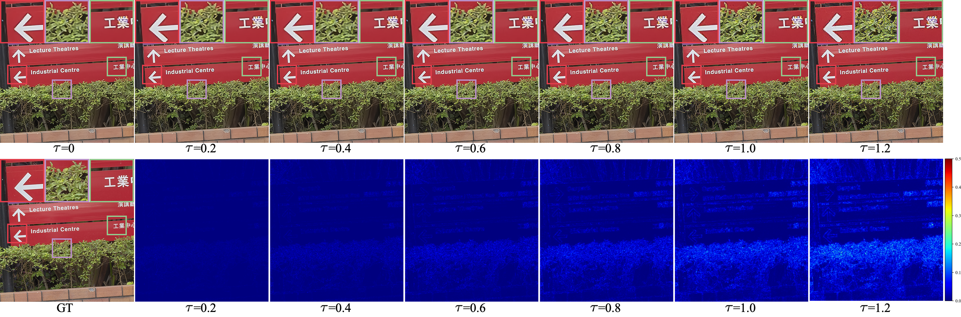
Here, we analyze the effects of the sampling temperature $\tau$ on SR performance of the proposed SDFlow in terms of PSNR and LPIPS. The sampling temperature controls the variance of the latent variable of the HF components when generating the SR image. As shown in Fig. (7), the decreased sampling temperature, i.e., $\tau<1$, increases the image quality in terms of LPIPS, and the best LPIPS is obtained when $\tau=0.8$. The sampling procedure becomes deterministic when $\tau$ decreases to 0, which achieves the best performance on the PSNR metric. However, the generated SR images are blurry as illustrated in Fig. (4). Increasing the sampling temperature leads to notable improvements in perceptual quality in terms of the LPIPS metric while degrades the distortion oriented PSNR metric. When the sampling temperature is set to larger than 1, we can observe a significant performance drop on the LPIPS and PSNR metric. Fig. (7) also shows the perception-distortion trade-off of the SR provided by the SDFlow, and it can be controlled by adjusting the sampling temperature.

References

- Yang and Huang [2017] Jianchao Yang and Thomas Huang. Image super-resolution: Historical overview and future challenges. In Super-resolution imaging, pages 1–34. CRC Press, 2017.
- Yang et al. [2019] Wenming Yang, Xuechen Zhang, Yapeng Tian, Wei Wang, Jing-Hao Xue, and Qingmin Liao. Deep learning for single image super-resolution: A brief review. IEEE Transactions on Multimedia, 21(12):3106–3121, 2019.
- Wang et al. [2020] Zhihao Wang, Jian Chen, and Steven CH Hoi. Deep learning for image super-resolution: A survey. IEEE Transactions on Pattern Analysis and Machine Intelligence, 43(10):3365–3387, 2020.
- Chen et al. [2022] Honggang Chen, Xiaohai He, Linbo Qing, Yuanyuan Wu, Chao Ren, Ray E Sheriff, and Ce Zhu. Real-world single image super-resolution: A brief review. Information Fusion, 79:124–145, 2022.
- Liu et al. [2022] Anran Liu, Yihao Liu, Jinjin Gu, Yu Qiao, and Chao Dong. Blind image super-resolution: A survey and beyond. IEEE Transactions on Pattern Analysis and Machine Intelligence, 2022.
- Wei et al. [2020] Pengxu Wei, Ziwei Xie, Hannan Lu, Zongyuan Zhan, Qixiang Ye, Wangmeng Zuo, and Liang Lin. Component divide-and-conquer for real-world image super-resolution. In European Conference on Computer Vision, 2020.
- Chen et al. [2019a] Chang Chen, Zhiwei Xiong, Xinmei Tian, Zheng-Jun Zha, and Feng Wu. Camera lens super-resolution. In IEEE Conference on Computer Vision and Pattern Recognition, 2019a.
- Cai et al. [2019] Jianrui Cai, Hui Zeng, Hongwei Yong, Zisheng Cao, and Lei Zhang. Toward real-world single image super-resolution: A new benchmark and a new model. In IEEE International Conference on Computer Vision, 2019.
- Chen et al. [2019b] Chang Chen, Zhiwei Xiong, Xinmei Tian, ZhengJun Zha, and Feng Wu. Camera lens super-resolution. In IEEE Conference on Computer Vision and Pattern Recognition, 2019b.
- Köhler et al. [2019] Thomas Köhler, Michel Bätz, Farzad Naderi, André Kaup, Andreas Maier, and Christian Riess. Toward bridging the simulated-to-real gap: Benchmarking super-resolution on real data. IEEE Transactions on Pattern Analysis and Machine Intelligence, 42(11):2944–2959, 2019.
- Joze et al. [2020] Hamid Reza Vaezi Joze, Ilya Zharkov, Karlton Powell, Carl Ringler, Luming Liang, Andy Roulston, Moshe Lutz, and Vivek Pradeep. Imagepairs: Realistic super resolution dataset via beam splitter camera rig. In IEEE Conference on Computer Vision and Pattern Recognition Workshops, pages 518–519, 2020.
- Sun et al. [2021] Wei Sun, Dong Gong, Qinfeng Shi, Anton van den Hengel, and Yanning Zhang. Learning to zoom-in via learning to zoom-out: Real-world super-resolution by generating and adapting degradation. IEEE Transactions on Image Processing, 30:2947–2962, 2021.
- Son et al. [2022] Sanghyun Son, Jaeha Kim, Wei-Sheng Lai, Ming-Hsuan Yang, and Kyoung Mu Lee. Toward real-world super-resolution via adaptive downsampling models. IEEE Transactions on Pattern Analysis and Machine Intelligence, 44(11):8657–8670, 2022.
- Wei et al. [2021] Yunxuan Wei, Shuhang Gu, Yawei Li, Radu Timofte, Longcun Jin, and Hengjie Song. Unsupervised real-world image super resolution via domain-distance aware training. In IEEE Conference on Computer Vision and Pattern Recognition, 2021.
- Maeda [2020] Shunta Maeda. Unpaired image super-resolution using pseudo-supervision. In IEEE Conference on Computer Vision and Pattern Recognition, 2020.
- Lugmayr et al. [2019] Andreas Lugmayr, Martin Danelljan, and Radu Timofte. Unsupervised learning for real-world super-resolution. In IEEE International Conference on Computer Vision Workshop, 2019.
- Fritsche et al. [2019] Manuel Fritsche, Shuhang Gu, and Radu Timofte. Frequency separation for real-world super-resolution. In IEEE International Conference on Computer Vision Workshop, 2019.
- Yuan et al. [2018] Yuan Yuan, Siyuan Liu, Jiawei Zhang, Yongbing Zhang, Chao Dong, and Liang Lin. Unsupervised image super-resolution using cycle-in-cycle generative adversarial networks. In IEEE Conference on Computer Vision and Pattern Recognition Workshops, 2018.
- Bulat et al. [2018] Adrian Bulat, Jing Yang, and Georgios Tzimiropoulos. To learn image super-resolution, use a gan to learn how to do image degradation first. In European Conference on Computer Vision, 2018.
- Goodfellow et al. [2014] Ian J Goodfellow, Jean Pouget-Abadie, Mehdi Mirza, Bing Xu, David Warde-Farley, Sherjil Ozair, Aaron C Courville, and Yoshua Bengio. Generative adversarial nets. In Advances in Neural Information Processing Systems, 2014.
- Romero et al. [2022] Andrés Romero, Luc Van Gool, and Radu Timofte. Unpaired real-world super-resolution with pseudo controllable restoration. In IEEE Conference on Computer Vision and Pattern Recognition, 2022.
- Wolf et al. [2021] Valentin Wolf, Andreas Lugmayr, Martin Danelljan, Luc Van Gool, and Radu Timofte. Deflow: Learning complex image degradations from unpaired data with conditional flows. In IEEE Conference on Computer Vision and Pattern Recognition, 2021.
- Ning et al. [2022] Qian Ning, Jingzhu Tang, Fangfang Wu, Weisheng Dong, Xin Li, and Guangming Shi. Learning degradation uncertainty for unsupervised real-world image super-resolution. In International Joint Conference on Artificial Intelligence, 2022.
- Luo et al. [2022] Zhengxiong Luo, Yan Huang, Shang Li, Liang Wang, and Tieniu Tan. Learning the degradation distribution for blind image super-resolution. In IEEE Conference on Computer Vision and Pattern Recognition, 2022.
- Lee et al. [2022] Sangyun Lee, Sewoong Ahn, and Kwangjin Yoon. Learning multiple probabilistic degradation generators for unsupervised real world image super resolution. In European Conference on Computer Vision Workshops, 2022.
- Dinh et al. [2015] Laurent Dinh, David Krueger, and Yoshua Bengio. NICE: non-linear independent components estimation. In International Conference on Learning Representations, 2015.
- Dinh et al. [2017] Laurent Dinh, Jascha Sohl-Dickstein, and Samy Bengio. Density estimation using real NVP. In International Conference on Learning Representations, 2017.
- Kingma and Dhariwal [2018] Durk P Kingma and Prafulla Dhariwal. Glow: Generative flow with invertible 1x1 convolutions. Advances in neural information processing systems, 31, 2018.
- Guo et al. [2020] Yong Guo, Jian Chen, Jingdong Wang, Qi Chen, Jiezhang Cao, Zeshuai Deng, Yanwu Xu, and Mingkui Tan. Closed-loop matters: Dual regression networks for single image super-resolution. In IEEE Conference on Computer Vision and Pattern Recognition, 2020.
- Xiao et al. [2020] Mingqing Xiao, Shuxin Zheng, Chang Liu, Yaolong Wang, Di He, Guolin Ke, Jiang Bian, Zhouchen Lin, and Tie-Yan Liu. Invertible image rescaling. In European Conference on Computer Vision, 2020.
- Liang et al. [2021a] Jingyun Liang, Andreas Lugmayr, Kai Zhang, Martin Danelljan, Luc Van Gool, and Radu Timofte. Hierarchical conditional flow: A unified framework for image super-resolution and image rescaling. In IEEE International Conference on Computer Vision, 2021a.
- Ji et al. [2020] Xiaozhong Ji, Yun Cao, Ying Tai, Chengjie Wang, Jilin Li, and Feiyue Huang. Real-world super-resolution via kernel estimation and noise injection. In IEEE Conference on Computer Vision and Pattern Recognition Workshops, 2020.
- Zhou and Susstrunk [2019] Ruofan Zhou and Sabine Susstrunk. Kernel modeling super-resolution on real low-resolution images. In IEEE International Conference on Computer Vision, 2019.
- Shocher et al. [2018] Assaf Shocher, Nadav Cohen, and Michal Irani. “zero-shot” super-resolution using deep internal learning. In IEEE Conference on Computer Vision and Pattern Recognition, 2018.
- Bell-Kligler et al. [2019] Sefi Bell-Kligler, Assaf Shocher, and Michal Irani. Blind super-resolution kernel estimation using an internal-gan. Advances in Neural Information Processing Systems, 32:284–293, 2019.
- Kim et al. [2020] Jonghee Kim, Chanho Jung, and Changick Kim. Dual back-projection-based internal learning for blind super-resolution. IEEE Signal Processing Letters, 27:1190–1194, 2020.
- Emad et al. [2021] Mohammad Emad, Maurice Peemen, and Henk Corporaal. DualSR: Zero-shot dual learning for real-world super-resolution. In IEEE Winter Conference on Applications of Computer Vision, 2021.
- Chen et al. [2023] Honggang Chen, Xiaohai He, Hong Yang, Yuanyuan Wu, Linbo Qing, and Ray E Sheriff. Self-supervised cycle-consistent learning for scale-arbitrary real-world single image super-resolution. Expert Systems with Applications, 212:118657, 2023.
- Kobyzev et al. [2020] Ivan Kobyzev, Simon JD Prince, and Marcus A Brubaker. Normalizing flows: An introduction and review of current methods. IEEE Transactions on Pattern Analysis and Machine Intelligence, 43(11):3964–3979, 2020.
- Ardizzone et al. [2019] Lynton Ardizzone, Jakob Kruse, Carsten Rother, and Ullrich Köthe. Analyzing inverse problems with invertible neural networks. In International Conference on Learning Representations, 2019.
- Lugmayr et al. [2020] Andreas Lugmayr, Martin Danelljan, Luc Van Gool, and Radu Timofte. Srflow: Learning the super-resolution space with normalizing flow. In European Conference on Computer Vision, 2020.
- Liang et al. [2021b] Jingyun Liang, Kai Zhang, Shuhang Gu, Luc Van Gool, and Radu Timofte. Flow-based kernel prior with application to blind super-resolution. In IEEE Conference on Computer Vision and Pattern Recognition, 2021b.
- Abdelhamed et al. [2019] Abdelrahman Abdelhamed, Marcus A Brubaker, and Michael S Brown. Noise flow: Noise modeling with conditional normalizing flows. In IEEE International Conference on Computer Vision, 2019.
- Yu et al. [2020] Jason J Yu, Konstantinos G Derpanis, and Marcus A Brubaker. Wavelet flow: Fast training of high resolution normalizing flows. Advances in Neural Information Processing Systems, 33:6184–6196, 2020.
- Xing et al. [2021] Yazhou Xing, Zian Qian, and Qifeng Chen. Invertible image signal processing. In IEEE Conference on Computer Vision and Pattern Recognition, 2021.
- Liu et al. [2021] Yang Liu, Zhenyue Qin, Saeed Anwar, Pan Ji, Dongwoo Kim, Sabrina Caldwell, and Tom Gedeon. Invertible denoising network: A light solution for real noise removal. In IEEE Conference on Computer Vision and Pattern Recognition, 2021.
- Zhao et al. [2021] Rui Zhao, Tianshan Liu, Jun Xiao, Daniel PK Lun, and Kin-Man Lam. Invertible image decolorization. IEEE Transactions on Image Processing, 30:6081–6095, 2021.
- Wang et al. [2021a] Xintao Wang, Liangbin Xie, Chao Dong, and Ying Shan. Real-esrgan: Training real-world blind super-resolution with pure synthetic data. In IEEE International Conference on Computer Vision, 2021a.
- Zhang et al. [2022] Wenlong Zhang, Guangyuan Shi, Yihao Liu, Chao Dong, and Xiao-Ming Wu. A closer look at blind super-resolution: Degradation models, baselines, and performance upper bounds. In IEEE Conference on Computer Vision and Pattern Recognition, 2022.
- Kingma and Welling [2014] Diederik P. Kingma and Max Welling. Auto-Encoding Variational Bayes. In International Conference on Learning Representations, 2014.
- Papamakarios et al. [2021] George Papamakarios, Eric Nalisnick, Danilo Jimenez Rezende, Shakir Mohamed, and Balaji Lakshminarayanan. Normalizing flows for probabilistic modeling and inference. The Journal of Machine Learning Research, 22(1):1–64, 2021.
- Wang et al. [2018] Xintao Wang, Ke Yu, Shixiang Wu, Jinjin Gu, Yihao Liu, Chao Dong, Yu Qiao, and Chen Change Loy. Esrgan: Enhanced super-resolution generative adversarial networks. In European Conference on Computer Vision Workshops, 2018.
- He et al. [2016] Kaiming He, Xiangyu Zhang, Shaoqing Ren, and Jian Sun. Deep residual learning for image recognition. In IEEE Conference on Computer Vision and Pattern Recognition, 2016.
- Zhang et al. [2023] Jize Zhang, Haolin Wang, Xiaohe Wu, and Wangmeng Zuo. Invertible network for unpaired low-light image enhancement. The Visual Computer, pages 1–12, 2023.
- Simonyan and Zisserman [2015] Karen Simonyan and Andrew Zisserman. Very deep convolutional networks for large-scale image recognition. In International Conference on Learning Representations, 2015.
- Ledig et al. [2017] Christian Ledig, Lucas Theis, Ferenc Huszár, Jose Caballero, Andrew Cunningham, Alejandro Acosta, Andrew Aitken, Alykhan Tejani, Johannes Totz, Zehan Wang, and Wenzhe Shi. Photo-realistic single image super-resolution using a generative adversarial network. In IEEE Conference on Computer Vision and Pattern Recognition, 2017.
- Mao et al. [2017] Xudong Mao, Qing Li, Haoran Xie, Raymond Y.K. Lau, Zhen Wang, and Stephen Paul Smolley. Least squares generative adversarial networks. In IEEE International Conference on Computer Vision, 2017.
- Grover et al. [2018] Aditya Grover, Manik Dhar, and Stefano Ermon. Flow-gan: Combining maximum likelihood and adversarial learning in generative models. In AAAI conference on artificial intelligence, volume 32, 2018.
- Wang et al. [2004] Zhou Wang, A.C. Bovik, H.R. Sheikh, and E.P. Simoncelli. Image quality assessment: from error visibility to structural similarity. IEEE Transactions on Image Processing, 13(4):600–612, 2004.
- Zhang et al. [2018] Richard Zhang, Phillip Isola, Alexei A. Efros, Eli Shechtman, and Oliver Wang. The unreasonable effectiveness of deep features as a perceptual metric. In IEEE Conference on Computer Vision and Pattern Recognition, 2018.
- Sheikh et al. [2005] H.R. Sheikh, A.C. Bovik, and G. de Veciana. An information fidelity criterion for image quality assessment using natural scene statistics. IEEE Transactions on Image Processing, 14(12):2117–2128, 2005.
- Mittal et al. [2013] Anish Mittal, Rajiv Soundararajan, and Alan C. Bovik. Making a “completely blind” image quality analyzer. IEEE Signal Processing Letters, 20(3):209–212, 2013.
- N et al. [2015] Venkatanath N, Praneeth D, Maruthi Chandrasekhar Bh, Sumohana S. Channappayya, and Swarup S. Medasani. Blind image quality evaluation using perception based features. In National Conference on Communications, 2015.
- Ma et al. [2017] Chao Ma, Chih-Yuan Yang, Xiaokang Yang, and Ming-Hsuan Yang. Learning a no-reference quality metric for single-image super-resolution. Computer Vision and Image Understanding, 158:1–16, 2017.
- Lugmayr et al. [2021] Andreas Lugmayr, Martin Danelljan, Radu Timofte, Christoph Busch, Yang Chen, Jian Cheng, Vishal Chudasama, Ruipeng Gang, Shangqi Gao, Kun Gao, Laiyun Gong, Qingrui Han, Chao Huang, Zhi Jin, Younghyun Jo, Seon Joo Kim, Younggeun Kim, Seungjun Lee, Yuchen Lei, Chu-Tak Li, Chenghua Li, Ke Li, Zhi-Song Liu, Youming Liu, Nan Nan, Seung-Ho Park, Heena Patel, Shichong Peng, Kalpesh Prajapati, Haoran Qi, Kiran Raja, Raghavendra Ramachandra, Wan-Chi Siu, Donghee Son, Ruixia Song, Kishor Upla, Li-Wen Wang, Yatian Wang, Junwei Wang, Qianyu Wu, Xinhua Xu, Sejong Yang, Zhen Yuan, Liting Zhang, Huanrong Zhang, Junkai Zhang, Yifan Zhang, Zhenzhou Zhang, Hangqi Zhou, Aichun Zhu, Xiahai Zhuang, and Jiaxin Zou. Ntire 2021 learning the super-resolution space challenge. In IEEE Conference on Computer Vision and Pattern Recognition Workshops, 2021.
- Ho et al. [2019] Jonathan Ho, Xi Chen, Aravind Srinivas, Yan Duan, and Pieter Abbeel. Flow++: Improving flow-based generative models with variational dequantization and architecture design. In International Conference on Machine Learning, 2019.
- Wang et al. [2021b] Wei Wang, Haochen Zhang, Zehuan Yuan, and Changhu Wang. Unsupervised real-world super-resolution: A domain adaptation perspective. In IEEE International Conference on Computer Vision, 2021b.
- Umer et al. [2020] Rao Muhammad Umer, Gian Luca Foresti, and Christian Micheloni. Deep generative adversarial residual convolutional networks for real-world super-resolution. In IEEE Conference on Computer Vision and Pattern Recognition Workshops, 2020.
- Lugmayr et al. [2022] Andreas Lugmayr, Martin Danelljan, Fisher Yu, Luc Van Gool, and Radu Timofte. Normalizing flow as a flexible fidelity objective for photo-realistic super-resolution. In IEEE Winter Conference on Applications of Computer Vision, 2022.
- Jinjin et al. [2020] Gu Jinjin, Cai Haoming, Chen Haoyu, Ye Xiaoxing, Jimmy S Ren, and Dong Chao. Pipal: a large-scale image quality assessment dataset for perceptual image restoration. In European Conference on Computer Vision, 2020.
- Heusel et al. [2017] Martin Heusel, Hubert Ramsauer, Thomas Unterthiner, Bernhard Nessler, and Sepp Hochreiter. Gans trained by a two time-scale update rule converge to a local nash equilibrium. In Advances in Neural Information Processing Systems, 2017.