Learning Individual Policies in Large Multi-agent Systems through Local Variance Minimization
Abstract
In multi-agent systems with large number of agents, typically the contribution of each agent to the value of other agents is minimal (e.g., aggregation systems such as Uber, Deliveroo). In this paper, we consider such multi-agent systems where each agent is self-interested and takes a sequence of decisions and represent them as a Stochastic Non-atomic Congestion Game (SNCG). We derive key properties for equilibrium solutions in SNCG model with non-atomic and also nearly non-atomic agents. With those key equilibrium properties, we provide a novel Multi-Agent Reinforcement Learning (MARL) mechanism that minimizes variance across values of agents in the same state. To demonstrate the utility of this new mechanism, we provide detailed results on a real-world taxi dataset and also a generic simulator for aggregation systems. We show that our approach reduces the variance in revenues earned by taxi drivers, while still providing higher joint revenues than leading approaches.
Introduction
In this paper, we are motivated by large scale multi-agent systems such as car matching systems (Uber, Lyft, Deliveroo etc.), food delivery systems (Deliveroo, Ubereats, Foodpanda, DoorDash etc.), grocery delivery systems (AmazonFresh, Deliv, RedMart etc) and traffic routing guidance. The individual agents need to make sequential decisions (e.g.,on where to position themselves) in the presence of uncertainty. The objective in aggregation systems is typically to maximize overall revenue and this can result in individual agent revenues getting sacrificed. Towards ensuring fair outcomes for individual agents, our focus in this paper is on enabling computation of approximate equilibrium solutions.
Competitive Multi-Agent Reinforcement Learning (MARL) (Littman 1994) with an objective of computing equilibrium is an ideal model for representing the underlying decision problem. There has been a significant amount of research on learning equilibrium policies in MARL problems (Littman 1994; Watkins and Dayan 1992; Hu, Wellman et al. 1998; Littman 2001). However, these approaches typically can scale to problems with few agents. Recently, there have been Deep Learning based MARL methods (Yu et al. 2021; Heinrich and Silver 2016; Yang et al. 2018; Lowe et al. 2017) that can scale to a large number of agents on account of using decentralized learning. While decentralized learning is scalable, such approaches consider all other agents in aggregate or as part of the environment and this can have an impact on overall effectiveness (as demonstrated in our experimental results).
To that end, we propose a Stochastic Non-atomic Congestion Game (SNCG) model, which combines Stochastic Game (Shapley 1953) and Non-atomic Congestion Game (NCG) models (Roughgarden and Tardos 2002; Krichene, Drighès, and Bayen 2015). SNCG helps exploit anonymity in interactions and minimal contribution of individual agents, which are key facets of aggregation systems of interest in this paper. More importantly, we use a key theoretical property of the SNCG model to design a novel model free multi-agent reinforcement learning approach that is suitable for both non-atomic and nearly non-atomic agents. Specifically, we prove that at equilibrium values of non-atomic agents, which are all in the same local state are equal. Our model free MARL approach, referred to as LVMQ (Local Variance Minimizing Q-learning) reduces variance in “best response” agent values in local states to move joint solutions towards equilibrium solutions.
We demonstrate the utility of our new approach for individual drivers on a large dataset from a major Asian city by comparing against leading decentralized learning approaches including Neural Fictitious Self Play (NFSP) (Heinrich and Silver 2016), Mean Field Q-learning (MFQ) (Yang et al. 2018) and Multi-Agent Actor Critic (MAAC) (Lowe et al. 2017). In addition, we also provide results on a general purpose simulator for aggregation systems.
Related work
The most relevant research is on computing equilibrium policies in MARL problems, which is represented as learning in stochastic games (Shapley 1953). Nash-Q learning (Hu, Wellman et al. 1998) is a popular algorithm that extends the classic single agent Q-learning (Watkins and Dayan 1992) to general sum stochastic games. In fictitious self play (FSP) (Heinrich, Lanctot, and Silver 2015) agents learn best response through self play. FSP is a learning framework that implements fictitious play (Brown 1951) in a sample-based fashion. There are a few works which assume existence of a potential function and either need to know the potential function a priori (Marden 2012) or estimate potential function’s value (Mguni 2020). Unfortunately, all these algorithms are generally suited for a few agents and do not scale if the number of agents is very large, which is the case for the problems of interest in this paper.
Recently, some deep learning based algorithms have been proposed to learn approximate Nash equilibrium in a decentralized manner. NFSP (Heinrich and Silver 2016) combines FSP with a neural network to provide a decentralized learning approach. Due to decentralization, NFSP is scalable and can work on problems with many agents. Centralized learning decentralized execution (CTDE) algorithms learn a centralized joint action value function during the training phase, however individual agents optimize their actions based on their local observation. MAAC (Lowe et al. 2017) is a CTDE algorithm which is a best response based learning method and does not focus on learning equilibrium policy. M3DDPG (Li et al. 2019) learn policies against altering adversarial policies by optimizing a minimax objective. SePS (Christianos et al. 2021) is another CTDE algorithm which focuses on parameter sharing to increase scalabilty of MARL. However these methods do not consider infinitesimal contribution of individual agents. As we demonstrate in our experimental results, our approach that benefits from exploiting key properties of SNCG is able to outperform NFSP and MAAC with respect to the quality of approximate equilibrium solutions on multiple benchmark problem domains from literature. There are some CTDE algorithms (Sunehag et al. 2018; Rashid et al. 2018; Yu et al. 2021) which focus on cooperative settings and not suitable for non-cooperative setting of our interest.
Treating large multi-agent systems as mean field game (MFG) (Huang, Caines, and Malhamé 2003) is a popular approach to solve large scale MARL problems where each agent learns to play against mean field distribution of all other agents. For MFQ (Yang et al. 2018), individual agents learn Q-values of its interaction with average action of its neighbour agents. (Hüttenrauch et al. 2019) used mean feature embeddings as state representations to encode the current distribution of the agents. (Subramanian et al. 2020) extended MFQ to multiple types of players. In the context of finite MFGs, (Cui and Koeppl 2021) proposed approximate solution approaches using entropy regularization and Boltzmann policies. Recently (Subramanian et al. 2022) proposed decentralized MFG where agents model the mean field during the training process. This thread of research is closely related to our work and we show that by utilizing extra information shared by the central agent, LVMQ outperforms MFQ.
We have proposed to minimize variance in the values of agents present in same local state to learn equilibrium policy. Some works in single agent reinforcement learning have focused on direct and indirect (Sherstan et al. 2018; Jain et al. 2021; Tamar, Di Castro, and Mannor 2016) approaches to compute variance in the return of a single agent. This is fundamentally different from LVMQ, where variance is across values of multiple agents present in a local state (instead of variance in value distribution for a single agent in those approaches).

Background: Non-atomic Congestion Game (NCG)
NCG has either been used to model selfish routing (Roughgarden and Tardos 2002; Roughgarden 2007; Fotakis et al. 2009) or resource sharing (Chau and Sim 2003; Krichene, Drighès, and Bayen 2015; Bilancini and Boncinelli 2016) problems. Here we present a brief overview of NCG (Krichene, Drighès, and Bayen 2015) from the perspective of resource sharing problem as that is of relevance to domains of interest, where taxis have to share demand in different zones.
In NCG, a finite set of resources are shared by a set of players . To capture the infinitesimal contribution of each agent, the set is endowed with a measure space: . is a -algebra of measurable subsets, is a finite Lebesgue measure and is interpreted as the mass of the agents. This measure is non-atomic, i.e., for a single agent set , . The set (with =1, i.e., mass of all agents is 1) is partitioned into populations, . Each population type possesses a set of strategies , and each strategy corresponds to a subset of the resources. Each agent selects a strategy, which leads to a joint strategy distribution, . Here is the total mass of the agents from population who choose strategy . The total consumption of a resource in a strategy distribution is given by:
The cost of using a resource for strategy is: where the function represents cost of congestion and is assumed to be a non-decreasing continuous function. The cost experienced by an agent of type which selects strategy is given by: . A strategy is a Nash equilibrium if:
Intuitively, it implies that the cost for any other strategy, will be greater than or equal to the cost of strategy, . It also implies that for a population , all the strategies with non-zero mass will have equal costs.
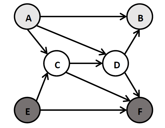
Packet routing problem in Figure 1a is an example of an NCG. Two agent populations () and of mass 0.5 each share the network. Each edge is treated as a resource. Agents from send packets from node to node , and the the agents from send from node to node . Paths (strategies) are available for population whereas paths are available for population . A joint strategy is said to be an equilibrium strategy if for population type , costs on paths available to them with non-zero mass are equal. Refer to the equilibrium policy given in Table 1, the costs on paths and (paths with non-zero mass) for population will be equal at equilibrium.
Stochastic Non-atomic Congestion Games (SNCG)
In this section we propose SNCG model, which is a combination of NCG and Stochastic Games. NCG is primarily for single stage settings, we extend it to multi-stage settings in SNCG. Formally, SNCG is the tuple:
-
:
set of agents with properties similar to the ones in NCG described in Section Background: Non-atomic Congestion Game (NCG).
-
:
set of local states for individual agents (e.g., location zone of a taxi).
-
:
set of global states (e.g., distributions of taxis in the city). At any given time, is divided into disjoint sets, , where is the set of agents present in local state in global state and is the mass of agents in . The distribution of mass of agents is considered as the global state, i.e., . The global state is continuous and total mass of agents in a global state is 1.
-
:
is the set of actions, where represents the set of actions (e.g., locations to move to) available to individual agents in the local state . . Let provides the action selected by agent . We define as the total mass of agents in selecting action in state , i.e. . If the agents are playing deterministic policies, is given by . Similar to NCG, joint action is the distribution of masses of agents selecting available actions in each local state, i.e. for state , .
-
: is the reward function111“cost” is often used in context of NCG. To be consistent with MARL literature we use the term “reward”., which can be assumed as negative of cost function of NCGs. The total mass of agents selecting action for a joint action in state is given by . refers to the vector of mass of agents selecting different actions. Similar to the cost functions in NCG, the reward function (-ve of cost) is assumed to be a non-increasing continuous function.
Depending on whether the congestion being represented is in source state of agent (node) or on the edge between two states, we have two possible reward cases of relevance in aggregation systems:
-
R1
: Reward dependent only on joint state, local state and joint action, i.e., . An example of this type of reward function would be referring to congestion at attractions in theme parks and individuals (agents) are minimizing their overall wait times.
-
R2
: Reward dependent on joint state, local state, joint action and local action, i.e., . This is useful in representing congestion related to traffic on roads. An example would be congestion on roads, where individual drivers are trying to reach their destination in the least time.
-
R1
-
: is the transitional probability of global states222Considering local transitions is simpler, as global transition can be computed from local transitions. given joint actions. Similar to reward function, transition of global state is also dependent on the total mass of agents selecting different actions in state .
In SNCG, each state is an instance of NCG where agents in a local state select actions available to them and the environment moves to the next state (another instance of NCG). Also, as the same set of actions are available to all the agents present in a given local state, agents present in the local state can be considered as agents of same population type. Figure 1b represents state transition from global state to for a simple grid-world with 2 zones and and total mass of agents is 1. The number in the grid represents mass of agents present in that zone, i.e. and . Each zone has two feasible actions, = stay in the current zone and = move to the next zone, i.e. . From NCG point of view, state is an NCG with 0.2 mass of agents of population type and 0.8 mass of agents of population type . Similarly, can be viewed as an NCG with 0.4 mass of agents of type and 0.6 mass of agents of type . Suppose 0.1 mass of agents in chose to stay and remaining chose to move to . Similarly, 0.48 mass of agents in selected to stay whereas remaining agents selected action and due to transition uncertainty, the environment moves to . The joint action (which is continuous) of the agents is given by .
The policy of agent is denoted by . We observe that given a global state , an agent will play different policies based on its local state as the available actions for local states are different. Hence, can be represented as . We define as the set of policies available to an agent in local state , hence, . is the joint policy of all the agents.
Let be the discount factor. The value of agent for being in local state given the global state is and other agents are following policy is given by (for the R2 reward case):
| (1) |
The goal is to compute an equilibrium joint strategy, where no individual agent has an incentive to unilaterally deviate.
Properties of equilibrium in SNCG
In this section, we show that values of agents in the same local state have either equal or close to equal values at equilibrium. We begin with the case of non-atomic agents and then move to the case with large number of agents and where mass of an agent is non-zero. Due to space constraints, we only provide proof sketches and the detailed proofs are provided in the appendix.
Non-Atomic Agents:
In case of non-atomic agents, we first prove that values of other agents do not change if only one agent changes its policy (Proposition 1). This property is then later used to prove that values of agents present in a local state are equal at equilibrium (Proposition 2).
Proposition 1.
Values of other agents do not change if agent alone changes its policy from to , i.e., for any agent in any local state : and
Proof Sketch. As can be observed in Equation 1, change of policy for agent can have impact on agent ’s value, , due to one common summary factor, which is the mass of agents taking a certain action in state with zone , .
Since is primarily mass of agents, which is a Lebesgue measure and using the countable additivity property of Lebesgue measure (Bogachev 2007; Hartman and Mikusinski 2014), we have:
Integral at a point in continuous space is 0 and mass measure is non-atomic, so is a null set and .
Based on Proposition 1, we now show that at Nash Equilibrium for SNCG, values of agents that are in same local state are equal. A joint policy is a Nash equilibrium if for all and for all , there is no incentive for anyone to deviate unilaterally, i.e.
Proposition 2.
Values of agents present in a local state are equal at equilibrium (denoted by *), i.e.,
Proof Sketch. In the proof of Proposition 1, we showed that adding or subtracting one agent from a local state does not change other agent’s values, as contribution of one agent is infinitesimal. Combining this with the equilibrium condition employed in NashQ learning (Hu and Wellman 2003) with local states, we have:
These results can also be extended to problems with multiple types of agents.
Corollary 1.
For problems with multiple types of agents, values of same type of agents are equal in a local state at equilibrium for non-atomic case. ∎
In non-atomic case, individual agents have zero mass and we have shown here that values of agents with same local states will be equal at equilibrium. We now move onto domains with large number of agents but not completely non-atomic. Since agents have non-zero mass, the proofs above do not directly hold.
Nearly Non-Atomic Agents:
In aggregation systems, there are many agents but each agent has a small amount of mass. For this case of nearly non-atomic agents, we are only able to provide the proof for reward setting R1.
Proposition 3.
When agents have non-zero mass in SNCG, consider two agents, and in zone and let be the equilibrium policy. For R1 setting, we have:
Proof Sketch. Since the joint policy, is the same for both and , and consequently are the same for both and . Therefore, is the same as it is defined on zone and not on individual action. Transition function is on joint state and action space, so we can recursively show that future values are also the same.
For the reward setting R2, we are only able to provide a trivial theoretical upper bound on the difference as shown in the appendix. Therefore, we empirically evaluate our hypothesis that values of agents in same state are equal with reward setting R2.
SNCG model requires transition and reward models, which are typically hard to have a priori. Hence, using the insight of Proposition 2, we provide a model free deep multi-agent learning approach to compute approximate equilibrium joint policies in multi-agent systems where there are large (yet finite) number of agents. We demonstrate in our experimental results, our solutions are better (both in terms of overall solution quality and reduction in revenue variance of all agents) than the leading approaches for MARL problems on multiple benchmark problems.
Local Variance minimizing Multi-agent Q-learning, LVMQ
Given the propositions in section Properties of equilibrium in SNCG for SNCGs, we hypothesize that values of all the agents present in any local state are equal at equilibrium (even for reward case R2) when there are a large number of agents with minor contributions from each agent (nearly non-atomic agents). This translates to having zero variance333We have used zero variance as an indicative of equal values of agents in the paper, however, other measures such as standard deviation can also be used for the same purpose. in individual agent values at each local state, while individual agents are playing their best responses. Please note that a joint policy which yields equal values in local states is an equilibrium policy only if agents are also playing their best response strategy. This is the key idea of our LVMQ approach and is an ideal insight for approximating equilibrium solutions in aggregation systems. The centralized entity can focus on ensuring values of agents in same local states are (close to) equal by estimating a joint policy which minimizes variance in values, while the individual suppliers can focus on computing best response solutions. During learning phase, the role of the
-
Central entity is to ensure that the exploration of individual agents moves towards a joint policy where the variance in values of agents in a local state is minimum.
-
Individual agents is to learn their best responses to the historical behaviour of the other agents based on guidance from central entity.
We now describe the four main steps of the algorithm.
Central agent suggests local variance minimizing joint action, to individual agents:
We employ policy gradient framework for central agent to learn a joint policy which minimizes variance in values of individual agents in local states.
Learning experience of the central agent is given by , where is the mean of variances in the current values of agents in local states, i.e., . represents the variance in values of agents in . We define two parameterized functions: joint policy function (joint policy which yields minimum variance in individual values) and variance function . Since the goal is to minimize variance, we need to update joint policy parameters in the negative direction of the gradient of , i.e., . The gradient for policy parameters can be computed using chain rule as follows
| (2) |
Individual agents play suggested or best response action: Individual agents either follow the suggested action with probability or play their best response policy with probability. While playing the best response policy, the individual agents explore with probability (i.e. fraction of probability) and with the remaining probability (() fraction of ) they play their best response action. Both the values are decayed exponentially. The individual agents maintain a network to approximate the best response to historical behavior of the other agents in local state when global state is . The learning experience of agent is given by .
Environment moves to the next state: All the individual agents observe their individual reward and update their best response values. Central agent observes the true-joint action performed by the individual agents. Based on the true joint-action and variance () in the values of agents, the central agent updates its own learning.
Compute loss functions and optimize value and policy: As common with deep RL methods (Mnih et al. 2015; Foerster et al. 2017), replay buffer is used to store experiences ( for the central agent and for individual agent ) and target networks (parameterized with ) are used to increase the stability of learning. We define , and as the loss functions of , and networks respectively. The loss values are computed based on mini batch of experiences as follows
is computed based on mean squared error, is computed based on TD error (Sutton 1988) and is computed based on the gradient provided in Equation 2. Using these loss functions, policy and value functions are optimized. We have provided detailed steps of LVMQ in the appendix.


Experiments
We perform experiments on three different domains, taxi simulator based on real-world and synthetic data set (Verma, Varakantham, and Lau 2019; Verma and Varakantham 2019), a single stage packet routing (Krichene, Drighes, and Bayen 2014) and multi-stage traffic routing (Wiering 2000). In all these domains a central agent that can assist (or provides guidance to) individual agents in approximating equilibrium policies is present. MARL strategy is suitable for these domains as these are large multi-agent systems where model based planning is not scalable. For taxi domain, we do not compare with other aggregation system related methods (Shah, Lowalekar, and Varakantham 2020; Lowalekar, Varakantham, and Jaillet 2018; Liu, Li, and Wu 2020) as these methods focus on joint value and disregard the fact that the individual drivers are self-interested. Different from these methods, we focus on learning from individual drivers’ perspective while considering that other drivers are also learning simultaneously.
We compare with four baseline algorithms: Independent Learner (IL), NFSP (Heinrich and Silver 2016), MFQ (Yang et al. 2018) and MAAC (Lowe et al. 2017). IL is a traditional Q-Learning algorithm that does not consider the actions performed by the other agents. Similar to LVMQ, MFQ and MAAC are also CTDE algorithms and they use joint action information at the time of training. However, NFSP is a self play learning algorithm and learns from individual agent’s local observation. Hence, for fair comparison, we provide joint action information to NFSP as well. As mentioned by (Verma and Varakantham 2019), we also observed that the original NFSP without joint action information performs worse that NFSP with joint action information. In LVMQ, the central agent learns from the collective experiences of the individual agents and suggests individuals based on this learning, whereas other algorithms receive information only about the joint action. This is one of the reasons of LVMQ performing better than other algorithms.
For decentralized learning, ideally each agent should maintain their own neural network. However, simulating thousands of learning agents at the same time requires extensive computational resources hence, we simulated 1000 agents by using 100 neural networks with 10 agents sharing a single network (providing agent id as one of the input to the network). Letting agents share a single network while providing agent id to the network is common when decentralized learning is done for a large number of agents (Yang et al. 2017, 2018). For all the individual agents, we performed -greedy exploration and it was decayed exponentially. Training was stopped once decays to 0.05. We experimented with different values of aniticipatory parameter for NFSP and 0.1 provided us the best results. The results are average over runs with 5 different random seeds.
Taxi Simulator:
We build a taxi simulator based on both real-world and synthetic data set. The data set is from a taxi company in a major Asian city. It contains information about trips (time stamp, origin/destination locations, duration, fare) and movement logs of taxi drivers (GPS locations, time stamp, driver id, status of taxi). We used methods described in (Verma et al. 2017) to determine the total number of zones (111) for the simulation. Each zone is considered as a local state. Then we used the real world data to compute the demand between two zones and the time taken to travel between the zones. For simulation, we computed proportional number of demand between any pair of zones based on the number of agents being used in the simulator.
We also perform experiments using synthetic data set to simulate different features such as: (a) Demand-to-Agent-Ratio (DAR): the average amount of demand per time step per agent; (b) trip pattern: the average length of trips can be uniform for all the zones or there can be few zones which get longer trips (non-uniform trip pattern); and (c) demand arrival rate: arrival rate of demand can either be static w.r.t. the time or it can vary with time (dynamic arrival rate).


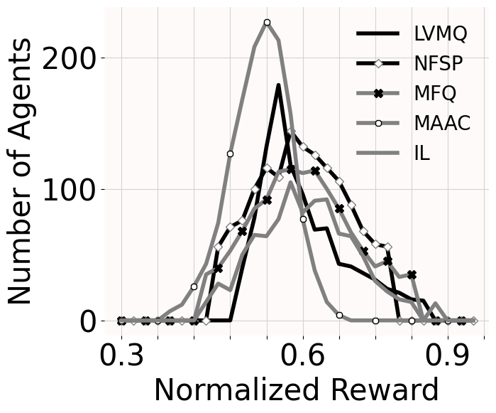
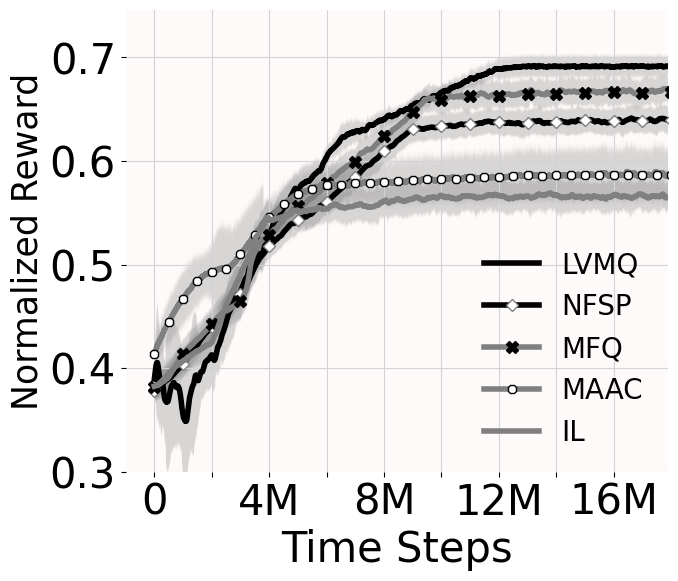
As agents try to maximize their long term revenue, we use mean reward of agents (w.r.t. the time) as the learning progresses as a comparison metric and show that LVMQ learns policy which yield higher mean values. The mean reward plots (2a-2d) are for the running average of mean payoff of all the agents for every (=1000) time steps. We also show variance in the values of agents after learning has converged. Plots 2e - 2h show distribution of values of agents in a zone. Though the zone with highest variance in values was not same for all the 5 algorithms, the top 5 zones with highest variance were almost same for these algorithms. Here we show values of agents in the selected zone over 2 time steps. We can see that the variance is minimum for LVMQ (evident from its narrower curve).
Figure 2a show that agents earn 5-10% more value for real-world data set (an improvement of 0.5% is considered a significant improvement (Xu et al. 2018) in aggregation systems) than NFSP, MFQ and MAAC. The mean reward for LVMQ is 3-5% more than the second best performing algorithm. The worst performance of IL is expected as it does not receive any extra information from the centralized agent.
Figure 2b plots mean reward of agents for a setup with dynamic arrival rate and non-uniform trip pattern with DAR=0.4. The mean reward for LVMQ is 4-10% higher that NFSP, MFQ and MAAC. Figures 2c show results for a setup with dynamic arrival rate, uniform trip pattern and DAR=0.5. Comparison for an experimental setup with static arrival rate, non-uniform trip pattern and DAR=0.6 is shown in Figure 2d. Treating IL as a baseline, the improvement (percentage increase in mean reward) achieved by LVMQ is 10-16%, NFSP is 5-12%, MFQ is 1-10% and MAAC is 1-6%. This means that LVMQ is able to capture lost-demand (able to serve demand before they expire). We also observed that the variance in values of individual agents was minimum for LVMQ. We discussed in Section Local Variance minimizing Multi-agent Q-learning, LVMQ that for a joint policy to be an equilibrium policy, agents should be playing their best responses in addition to having equal values (zero variance) in same local states. As agents are playing their best response policy and variance in values is low as compared to other algorithms, LVMQ learns policies that are closer to an equilibrium policy.
Packet Routing:
To compare the performance with exact equilibrium solution, we performed experiments with a single stage (exact equilibrium values for single stage can be computed using linear programming) packet routing game (Krichene, Drighes, and Bayen 2014) explained in Section Background: Non-atomic Congestion Game (NCG) (Figure 1a). The cost incurred on a path is the sum of costs on all the edges in the path. The costs functions for the edges when mass of population on the edge is are given by: ,
If the cost functions are known, exact equilibrium policy can be computed by minimizing non-atomic version (Krichene, Drighès, and Bayen 2015) of Rosenthal potential function (Rosenthal 1973). We use the exact equilibrium policy and corresponding costs to compare quality of the policy learned. We also compute epsilon (epsilon as in epsilon-equilibrium (Radner 1980)) values of the learned policy, which is the maximum reduction in cost of an agent when it changes its policy unilaterally. Table 1 compares the policies and epsilon values where the first row contain values computed using potential minimization method. In the table, the policy is represented as , where is the fraction of the population of type selecting path . We see that LVMQ policy is closest to the equilibrium policy and epsilon value is also lowest for it.
The equilibrium cost on paths computed by the potential minimization method are: . Figure 3a provide variance in costs of agents for both the population type. We can see that not only is the variance in the costs of agents minimum for LVMQ but the values are also very close to the values for exact equilibrium. We observed that other algorithms were able to perform similar to LVMQ if there is a clear choice of path based on their cost functions (the cost on one of the paths is very low such that it is advantageous for everyone to select that path). However, when complexity is increased by designing the cost function such that the choice is not very clear (see appendix), we observed that LVMQ starts outperforming other algorithms. The better performance of LVMQ is due to its advantage of receiving suggestions from a learned central agent.
| Method | policy | epsilon value |
|---|---|---|
| Equilibrium | ((0, 0.187, 0.813), | 0 |
| Policy | (0.223, 0.053, 0.724)) | |
| LVMQ | ((0, 0.187, 0.813), | 0.023 |
| (0.224, 0.045, 0.731)) | ||
| NFSP | ((0, 0.122, 0.878), | 0.342 |
| (0.005, 0.148, 0.847)) | ||
| MFQ | ((0, 0.171, 0.829), | 0.110 |
| (0.210, 0.040, 0.750)) | ||
| MAAC | ((0, 0.170, 0.830), | 0.140 |
| (0.201, 0.035, 0.764)) | ||
| IL | ((0, 0.219, 0.781), | 0.129 |
| (0.215, 0.048, 0.737)) |
Multi-Stage Traffic Routing:
We use the same network provided in Figure 1a to depict a traffic network where two population of agents and navigate from node to node and from node to node respectively. Unlike to the packet routing example, agents decide about their next edge at every node. Hence it is an example of SNCG and the values of agents from a population at a given node would be equal at equilibrium.
In this example, agents perform episodic learning and the episode ends when the agent reaches its destination node. The distribution of mass of population over the nodes is considered as state. Figure 3b shows that the variance in values of both the population type is minimum for LVMQ. Furthermore, we notice that for both single-stage and multi-stage cases, the setup is similar for agent population . However, for agents from , the values will be different from single-stage case. For example, agents selecting path and will reach the destination node at different time steps and hence cost of agents on edge will be different from the single-stage case. Hence we can safely assume that the equilibrium value of agents from population will be 1.22 (as computed for the single-stage case) which is the value for LVMQ as shown in Figure 3b.
Conclusion
We propose a Stochastic Non-atomic Congestion Games (SNCG) model to represent anonymity in interactions and infinitesimal contribution of individual agents for aggregation systems. We show that the values of all the agents present in a local state are equal at equilibrium in SNCG. Based on this property we propose LVMQ which is a CTDE algorithm to learn approximate equilibrium policies in cases with finite yet large number of agents. Experimental results on multiple domains depict that LVMQ learns better equilibrium policies than other state-of-the-art algorithms.
References
- Bilancini and Boncinelli (2016) Bilancini, E.; and Boncinelli, L. 2016. Strict Nash equilibria in non-atomic games with strict single crossing in players (or types) and actions. Economic Theory Bulletin, 4(1): 95–109.
- Bogachev (2007) Bogachev, V. I. 2007. Measure theory, volume 1. Springer Science & Business Media.
- Brown (1951) Brown, G. W. 1951. Iterative solution of games by fictitious play. Activity analysis of production and allocation, 13: 374–376.
- Chau and Sim (2003) Chau, C. K.; and Sim, K. M. 2003. The price of anarchy for non-atomic congestion games with symmetric cost maps and elastic demands. Operations Research Letters, 31(5): 327–334.
- Christianos et al. (2021) Christianos, F.; Papoudakis, G.; Rahman, M. A.; and Albrecht, S. V. 2021. Scaling multi-agent reinforcement learning with selective parameter sharing. In International Conference on Machine Learning, 1989–1998. PMLR.
- Cui and Koeppl (2021) Cui, K.; and Koeppl, H. 2021. Approximately solving mean field games via entropy-regularized deep reinforcement learning. In International Conference on Artificial Intelligence and Statistics, 1909–1917. PMLR.
- Foerster et al. (2017) Foerster, J.; Nardelli, N.; Farquhar, G.; Afouras, T.; Torr, P. H.; Kohli, P.; and Whiteson, S. 2017. Stabilising experience replay for deep multi-agent reinforcement learning. In Proceedings of the 34th International Conference on Machine Learning-Volume 70, 1146–1155. JMLR. org.
- Fotakis et al. (2009) Fotakis, D.; Kontogiannis, S.; Koutsoupias, E.; Mavronicolas, M.; and Spirakis, P. 2009. The structure and complexity of Nash equilibria for a selfish routing game. Theoretical Computer Science, 410(36): 3305–3326.
- Hartman and Mikusinski (2014) Hartman, S.; and Mikusinski, J. 2014. The theory of Lebesgue measure and integration. Elsevier.
- Heinrich, Lanctot, and Silver (2015) Heinrich, J.; Lanctot, M.; and Silver, D. 2015. Fictitious self-play in extensive-form games. In International Conference on Machine Learning (ICML), 805–813.
- Heinrich and Silver (2016) Heinrich, J.; and Silver, D. 2016. Deep reinforcement learning from self-play in imperfect-information games. arXiv preprint arXiv:1603.01121.
- Hu and Wellman (2003) Hu, J.; and Wellman, M. P. 2003. Nash Q-learning for general-sum stochastic games. Journal of machine learning research, 4(Nov): 1039–1069.
- Hu, Wellman et al. (1998) Hu, J.; Wellman, M. P.; et al. 1998. Multiagent reinforcement learning: theoretical framework and an algorithm. In ICML, volume 98, 242–250. Citeseer.
- Huang, Caines, and Malhamé (2003) Huang, M.; Caines, P. E.; and Malhamé, R. P. 2003. Individual and mass behaviour in large population stochastic wireless power control problems: centralized and Nash equilibrium solutions. In 42nd IEEE International Conference on Decision and Control (IEEE Cat. No. 03CH37475), volume 1, 98–103. IEEE.
- Hüttenrauch et al. (2019) Hüttenrauch, M.; Adrian, S.; Neumann, G.; et al. 2019. Deep reinforcement learning for swarm systems. Journal of Machine Learning Research, 20(54): 1–31.
- Jain et al. (2021) Jain, A.; Patil, G.; Jain, A.; Khetarpal, K.; and Precup, D. 2021. Variance penalized on-policy and off-policy actor-critic. AAAI.
- Krichene, Drighes, and Bayen (2014) Krichene, W.; Drighes, B.; and Bayen, A. M. 2014. Learning nash equilibria in congestion games. arXiv preprint arXiv:1408.0017.
- Krichene, Drighès, and Bayen (2015) Krichene, W.; Drighès, B.; and Bayen, A. M. 2015. Online learning of nash equilibria in congestion games. SIAM Journal on Control and Optimization, 53(2): 1056–1081.
- Li et al. (2019) Li, S.; Wu, Y.; Cui, X.; Dong, H.; Fang, F.; and Russell, S. 2019. Robust multi-agent reinforcement learning via minimax deep deterministic policy gradient. In Proceedings of the AAAI Conference on Artificial Intelligence, volume 33, 4213–4220.
- Littman (1994) Littman, M. L. 1994. Markov games as a framework for multi-agent reinforcement learning. In Machine learning proceedings 1994, 157–163.
- Littman (2001) Littman, M. L. 2001. Friend-or-foe Q-learning in general-sum games. In International Conference on Machine Learning (ICML), volume 1, 322–328.
- Liu, Li, and Wu (2020) Liu, Z.; Li, J.; and Wu, K. 2020. Context-Aware Taxi Dispatching at City-Scale Using Deep Reinforcement Learning. IEEE Transactions on Intelligent Transportation Systems.
- Lowalekar, Varakantham, and Jaillet (2018) Lowalekar, M.; Varakantham, P.; and Jaillet, P. 2018. Online spatio-temporal matching in stochastic and dynamic domains. Artificial Intelligence, 261: 71–112.
- Lowe et al. (2017) Lowe, R.; Wu, Y.; Tamar, A.; Harb, J.; Abbeel, O. P.; and Mordatch, I. 2017. Multi-agent actor-critic for mixed cooperative-competitive environments. In Advances in Neural Information Processing Systems, 6379–6390.
- Marden (2012) Marden, J. R. 2012. State based potential games. Automatica, 48(12): 3075–3088.
- Mguni (2020) Mguni, D. 2020. Stochastic potential games. arXiv preprint arXiv:2005.13527.
- Mnih et al. (2015) Mnih, V.; Kavukcuoglu, K.; Silver, D.; Rusu, A. A.; Veness, J.; Bellemare, M. G.; Graves, A.; Riedmiller, M.; Fidjeland, A. K.; Ostrovski, G.; et al. 2015. Human-level control through deep reinforcement learning. Nature, 518(7540): 529–533.
- Radner (1980) Radner, R. 1980. Collusive behavior in noncooperative epsilon-equilibria of oligopolies with long but finite lives. Journal of economic theory, 22(2): 136–154.
- Rashid et al. (2018) Rashid, T.; Samvelyan, M.; Schroeder, C.; Farquhar, G.; Foerster, J.; and Whiteson, S. 2018. Qmix: Monotonic value function factorisation for deep multi-agent reinforcement learning. In International Conference on Machine Learning, 4295–4304. PMLR.
- Rosenthal (1973) Rosenthal, R. W. 1973. A class of games possessing pure-strategy Nash equilibria. International Journal of Game Theory, 2(1): 65–67.
- Roughgarden (2007) Roughgarden, T. 2007. Routing games. Algorithmic game theory, 18: 459–484.
- Roughgarden and Tardos (2002) Roughgarden, T.; and Tardos, É. 2002. How bad is selfish routing? Journal of the ACM (JACM), 49(2): 236–259.
- Shah, Lowalekar, and Varakantham (2020) Shah, S.; Lowalekar, M.; and Varakantham, P. 2020. Neural approximate dynamic programming for on-demand ride-pooling. In Proceedings of the AAAI Conference on Artificial Intelligence, volume 34, 507–515.
- Shapley (1953) Shapley, L. S. 1953. Stochastic games. Proceedings of the national academy of sciences, 39(10): 1095–1100.
- Sherstan et al. (2018) Sherstan, C.; Ashley, D. R.; Bennett, B.; Young, K.; White, A.; White, M.; and Sutton, R. S. 2018. Comparing Direct and Indirect Temporal-Difference Methods for Estimating the Variance of the Return. In UAI, 63–72.
- Subramanian et al. (2020) Subramanian, S. G.; Poupart, P.; Taylor, M. E.; and Hegde, N. 2020. Multi type mean field reinforcement learning. arXiv preprint arXiv:2002.02513.
- Subramanian et al. (2022) Subramanian, S. G.; Taylor, M. E.; Crowley, M.; and Poupart, P. 2022. Decentralized Mean Field Games. In Proceedings of the AAAI Conference on Artificial Intelligence, volume 36, 9439–9447.
- Sunehag et al. (2018) Sunehag, P.; Lever, G.; Gruslys, A.; Czarnecki, W. M.; Zambaldi, V.; Jaderberg, M.; Lanctot, M.; Sonnerat, N.; Leibo, J. Z.; Tuyls, K.; et al. 2018. Value-decomposition networks for cooperative multi-agent learning. AAMAS.
- Sutton (1988) Sutton, R. S. 1988. Learning to predict by the methods of temporal differences. Machine learning, 3(1): 9–44.
- Tamar, Di Castro, and Mannor (2016) Tamar, A.; Di Castro, D.; and Mannor, S. 2016. Learning the variance of the reward-to-go. The Journal of Machine Learning Research, 17(1): 361–396.
- Verma and Varakantham (2019) Verma, T.; and Varakantham, P. 2019. Correlated Learning for Aggregation Systems. Uncertainity in Artificial Intelligence (UAI).
- Verma et al. (2017) Verma, T.; Varakantham, P.; Kraus, S.; and Lau, H. C. 2017. Augmenting decisions of taxi drivers through reinforcement learning for improving revenues. International Conference on Automated Planning and Scheduling (ICAPS).
- Verma, Varakantham, and Lau (2019) Verma, T.; Varakantham, P.; and Lau, H. C. 2019. Entropy based Independent Learning in Anonymous Multi-Agent Settings. International Conference on Automated Planning and Scheduling (ICAPS).
- Watkins and Dayan (1992) Watkins, C. J.; and Dayan, P. 1992. Q-learning. Machine learning, 8(3-4): 279–292.
- Wiering (2000) Wiering, M. 2000. Multi-agent reinforcement learning for traffic light control. In Machine Learning: Proceedings of the Seventeenth International Conference (ICML’2000), 1151–1158.
- Xu et al. (2018) Xu, Z.; Li, Z.; Guan, Q.; Zhang, D.; Li, Q.; Nan, J.; Liu, C.; Bian, W.; and Ye, J. 2018. Large-scale order dispatch in on-demand ride-hailing platforms: A learning and planning approach. In Proceedings of the 24th ACM SIGKDD International Conference on Knowledge Discovery & Data Mining, 905–913.
- Yang et al. (2018) Yang, Y.; Luo, R.; Li, M.; Zhou, M.; Zhang, W.; and Wang, J. 2018. Mean Field Multi-Agent Reinforcement Learning. In International Conference on Machine Learning (ICML), 5567–5576.
- Yang et al. (2017) Yang, Y.; Yu, L.; Bai, Y.; Wang, J.; Zhang, W.; Wen, Y.; and Yu, Y. 2017. A study of ai population dynamics with million-agent reinforcement learning. arXiv preprint arXiv:1709.04511.
- Yu et al. (2021) Yu, C.; Velu, A.; Vinitsky, E.; Wang, Y.; Bayen, A.; and Wu, Y. 2021. The surprising effectiveness of mappo in cooperative, multi-agent games. arXiv preprint arXiv:2103.01955.
Supplementary Material
Properties of SNCG
In this section, we show that values of agents in the same local state have either equal or close to equal values at equilibrium. We begin with the case of non-atomic agents and then move to the case with large number of agents and where mass of an agent is non-zero.
Non-Atomic Agents
In case of non-atomic agents, we first prove that values of other agents do not change if only one agent changes its policy (Proposition 1). This property is then later used to prove that values of agents present in a local state are equal at equilibrium (Proposition 2).
Proposition 1.
Values of other agents do not change if agent alone changes its policy from to , i.e., for any agent in any local state : and
Proof.
As can be observed in the value function equation (Equation 1 in the main paper), change of policy for agent can have impact on agent ’s value, , due to the following three components:
immediate reward, i.e., ; or
transition function, i.e., ; or
future value,
All three components are dependent on one common summary factor, which is the mass of agents taking a certain action in state with zone . We will refer to this as (we are using to indicate that it is a change from original number of agents, ). Due to change in policy of , the number of agents taking an action in a zone can either increase or decrease. Without loss of generality, let us assume agent is using a deterministic policy444If agent employs a stochastic policy, the mass argument used in this proof is still applicable..
If change in policy moves agent away from zone , then the new mass of agents taking action in zone is
Since is primarily mass of agents, which is a Lebesgue measure and using the countable additivity property of Lebesgue measure (Bogachev 2007; Hartman and Mikusinski 2014), we have:
Similarly if change in agent policy implies moving into zone , the new value of number of agents taking action will be:
Since integral at a point in continuous space is 0 and mass measure is non-atomic, so is a null set and , and hence, . Since for any given and , none of the three components (immediate reward, transition function and future value) change. ∎
Based on Proposition 1, we now show that at Nash Equilibrium for SNCG, values of agents that are in same local state are equal. A joint policy is a Nash equilibrium if for all and for all , there is no incentive for anyone to deviate unilaterally, i.e.
Proposition 2.
Values of agents present in a local state are equal at equilibrium, i.e.,
| (3) |
where superscript * denotes equilibrium policies.
Proof.
In the proof of Proposition 1, we showed that adding or subtracting one agent from a local state does not change other agent’s values, as contribution of one agent is infinitesimal. Thus,
| (4) |
From equilibrium condition (value of equilibrium strategy is greater than or equal to value of any other strategy for each agent in every state) employed in NashQ learning (Hu and Wellman 2003) and the above results from Proposition 1, we have (accounting for local states):
Since the set of policies available to each agent are the same in each local state, i.e. one of the possible values of is and similarly one of the possible values of is . Hence
Since agents do not have specific identity (i.e., rewards are dependent on zone, transitions are on joint state), and are interchangeable. The above set of equations are only feasible if agent and in same local state have equal values, i.e.,
| Therefore: | ||||
∎
Corollary 2.
For problems with multiple types of agents, values of same type of agents are equal in a local state at equilibrium for non-atomic case.
In non-atomic case, individual agents have zero mass and we have shown here that values of agents with same local states will be equal at equilibrium. We now move onto domains with large number of agents but not completely non-atomic. Since agents have non-zero mass, the proofs above do not hold.
Nearly Non-atomic
In aggregation systems, where there are large number of agents but each agent has a small mass, we provide proofs for two reward cases separately.
Proposition 3.
Consider two agents, and in zone , and let be the equilibrium policy. For R1 setting, we have:
Proof.
We show this using mathematical induction on the horizon, .
For t = 1:
It should be noted that
Therefore, and hence
∎
Let us assume that it holds for , i.e.,
For , we have
| Similar to t = 1, we have and hence and . Given this and our assumption above, we have: | ||||
| (5) | ||||
For infinite horizon problems, we can just write this as
For reward case, R2 and nearly non-atomic agents, we are unable to provide a proof of value equivalence for agents in same local state. However, we can provide an upper bound on the difference value of any two agents in a given zone .
Let assume that for nearly non-atomic case, the maximum impact an agent can have in terms of reward at a time step is bounded by , i.e.,
| (6) |
This is a fair assumption, since there are a large number of agents in the nearly non-atomic case and each agent has a minimal impact.
For an equilibrium policy,, the difference in values of any two agents, and in the same zone is given
| It should be noted that and therefore the transition function values, will be the same for both agents. Next we substitute Equation 6 and use the sum of geometric progression to obtain (for infinite horizon case) | ||||
| (7) | ||||
For the finite horizon case, it will be (assuming there is no discount factor).
Local Variance minimizing Multi-agent Q-learning, LVMQ
Algorithm 1 provides detailed steps of LVMQ.
Hyperparameters
Our neural network consists of one hidden layer with 256 nodes. We also use dropout layer and layer normalization to prevent the network from overfitting. We ran our experiments on a 64-bit Ubuntu machine with 256G memory and used tensorflow for deep learning framework. We performed hyperparameter search for learning rate (1e-3 - 1e-5) and anticipatory parameter (0.1 - 0.8 for NFSP). The dropout rate was set to 50%. We used Adam optimizer for all the experimental domains. Learning rate was set to 1e-5 for all the experiments. Our learning rate is smaller than the rates generally used. We believe having low learning rate helps in dealing with non-stationarity when there are large number of agents present. We used 0, 1, 2022, 5e3, 1e5 as random seeds for 5 different runs of experiment.
Description of Simulator
The real-world data set is from a taxi company in a major Asian city which we will share after the paper is published. Demands (for both real-world and synthetic data set) are generated with a time-to-live value and the demand expires if it is not served within this time periods. Agents start at random zones and based on their learned policy move across the zones if no demand has been assigned to them. At every time step, the simulator assigns a trip probabilistically to the agents based on the number of agents present at the zone and the customer demand in that zone. Once a trip is assigned to an agent, it follows a fixed path to the destination and is no longer considered a candidate for a new trip. The agent starts following the learned policy only after it has completed the trip and is again ready to serve new trips. The fare of the trip minus the cost of traveling is used as the immediate reward for actions. The learning is episodic and an episode ends after every time steps.
Discussion on number of agents
LVMQ is motivated from the equilibrium property of having same value (i.e. zero variance) in a local state of SNCG. However, SNCG considers agents to be non-atomic. To check how many number of agents are required to consider an agent to be nearly non-atomic, we performed ablation study with different number of agents. Figure 4 provides results when we simulated the taxi domain using real world dataset with 20, 100, 200 and 1000 agents. Though the average reward is still higher for LVMQ, the variance and standard deviation is relatively high when there are 20 agents (Figures 4a and 4e). The values improve when 100 agents are used. It is evident from Figures 4c, 4g, 4d and 4h that LVMQ performs well when number of agent is around 200. Hence, we feel that we can approximate non-atomic behaviour when total number of agents are more than 200.


Packet Routing

Figure 5 shows another example of packet routing domain where two different populations of agents and of mass 0.5 each share the routing network. Population sends packets from node A to node B and population sends from node F to node G. AB, ADB, ACDB and ACEB are the paths available to population , whereas paths FG, FEG, FCEG and FCDG are available to population .
We now explain two examples where we used different cost functions to vary the complexity of learning. For example 1, the costs functions are such that both the populations do not share any edge at equilibrium. For the second example, the costs functions are selected in a way such that all the edges have non-zero mass of agents at equilibrium.
Example 1

The costs functions are as follows
Please notice that the cost function of AB is significantly lower than the other paths available to population . We use to represent the policy where is the fraction of the population of type selecting path . The exact equilibrium computed by solving LP (minimizing the potential function) is and the corresponding costs on each paths are as follows
We can see that costs on paths with zero mass (ex. ADB, ACDB, ACEB) are higher than the costs on paths with non-zero mass (AB) of agents. Also, costs on path with non-zero mass (ex. FG, FCDG) are equal at equilibrium.
| Method | epsilon value for example 1 | epsilon value for example 2 |
| LVMQ | 0.01 | 0.07 |
| NFSP | 0.02 | 0.44 |
| MFQ | 0.46 | 0.47 |
| MAAC | 0.03 | 0.57 |
| IL | 0.11 | 0.79 |
Example 2
Following are the cost functions
The exact equilibrium computed for this example is and corresponding costs on each path are

Figures 6 and 7 show variance in individual agents for examples 1 and 2 respectively. On the axis, means the variance is for population type for the corresponding algorithm. Table 2 contain the epsilon values (the maximum reduction in the cost of an agent when it changes its policy unilaterally) for both the examples.
We observe that all the algorithms learn near equilibrium policy for example 1 (specifically the policy of population ) and epsilon values are also low. However, LVMQ performs better than other algorithms for the second example. The variance is minimum for LVMQ and the epsilon value is also very low for it. Hence, LVMQ is able to learn policies which are close to equilibrium when complexity of learning is high.
Limitation
One limitation of LVMQ is its inability to distinguish between good equilibrium policy (high value) and bad equilibrium policy (low value) when multiple equilibria exists. Hence, LVMQ might converge towards the low value equilibrium policy if there are multiple equilibria.
From aggregation domain perspective, another limitation is that the work does not consider dynamic population of agents. The assumption is that the mass of agents remains trough out the learning episode ( time steps). However, in reality agents (taxi drivers) keep leaving/joining the environment and this may affect the learning performance if there is a significant rise/drop in overall mass of agents. We also do not consider heterogeneous agents and assume that utilities of all the agents are uniform. In reality, utility of same trip (though immediate reward is same) might be different for different agents.
Above mentioned limitations are separate research topics and we will explore these directions in our future work.