0.8pt
Learning Flock: Enhancing Sets of Particles for Multi Sub-State Particle Filtering with Neural Augmentation
Abstract
A leading family of algorithms for state estimation in dynamic systems with multiple sub-states is based on PFs. PFs often struggle when operating under complex or approximated modelling (necessitating many particles) with low latency requirements (limiting the number of particles), as is typically the case in multi target tracking (MTT). In this work, we introduce a deep neural network (DNN) augmentation for PFs termed LF. LF learns to correct a particles-weights set, which we coin flock, based on the relationships between all sub-particles in the set itself, while disregarding the set acquisition procedure. Our proposed LF, which can be readily incorporated into different PFs flow, is designed to facilitate rapid operation by maintaining accuracy with a reduced number of particles. We introduce a dedicated training algorithm, allowing both supervised and unsupervised training, and yielding a module that supports a varying number of sub-states and particles without necessitating re-training. We experimentally show the improvements in performance, robustness, and latency of LF augmentation for radar multi-target tracking, as well its ability to mitigate the effect of a mismatched observation modelling. We also compare and illustrate the advantages of LF over a state-of-the-art DNN-aided PF, and demonstrate that LF enhances both classic PFs as well as DNN-based filters.
I Introduction
The tracking of a time-evolving hidden state from noisy measurements is a fundamental signal processing task. \Acppf are a family of algorithms that allow tracking in (possibly) non-linear and non-Gaussian dynamic systems [2]. PFs naturally support tracking a single state, as well as a state comprised of multiple sub-states, i.e., MTT. Such filters are widely popular, and are utilized in many areas, ranging from robotics [3], through communication [4], and to positioning [5] and radar tracking [6, 7, 8].
PFs employ Monte Carlo simulation to iteratively update a set of samples coined particles, that represent sampling points of a continuous probability density function (PDF), and their corresponding weights, which represent their relative correctness [9, Ch. 12]. Their update is done according to a sequence of observations and the statistical modelling of the state evolution and the measurements, via different sampling-based stochastic procedures. While this operation enables the tracking of complex distributions, it also gives rise to increased complexity due to the need to maintain a large number of particles; and sensitivity to lacking or mismatched knowledge of the related models, that affects the update of the particles and may limit application in real-time systems [10]. To tackle these challenges, PFs often employ, e.g., adaptation of the number of particles [11, 12], robust designs [13, 14], or intricate sampling and resampling realizations [15, 16, 17, 7, 8], typically at the cost of increased complexity and latency and/or reduced performance.
Over the last decade, DNNs have emerged as powerful data-driven tools, that allow learning complex and abstract mappings from data [18]. The dramatic success of deep learning in domains such as computer vision and natural language processing has also lead to a growing interest in its combination with classic signal processing algorithms via model-based deep learning [19, 20, 21]. For tracking in dynamic systems, DNN-aided implementations of Kalman-type filters, that are typically suitable for tracking a single state in a Gaussian dynamic system, were studied in [22, 23, 24, 25, 26, 27].
In the context of PFs, various approaches were proposed in the literature to incorporate deep learning [28, 29, 30, 31, 32, 33, 34, 35]. In the last few years, arguably the most common approach uses DNNs to learn the sampling distribution, from which the particles are then individually sampled [28, 31, 30, 29, 32, 33, 34]. This can be done via supervised [28, 29, 30] and unsupervised [31, 32, 33, 34] learning. The latter is typically done by imposing a specific distribution model on the signals [31, 32, 33], thus inducing limitations when this assumption is violated. Alternatively, one can learn by mimicking each particle of another PF with the same number of particles that is considered accurate [34], and thus be bounded by its reference performance, which is often restrictive when operating with a limited number of particles. In multi sub-state settings, DNNs were used mainly as preprocessing [35], less so as an integral part of the PF flow. While the above existing neural augmentations were shown to enhance PFs, their design is typically tailored to a specific task, limiting transferability to other filters. Moreover, they operate in a per-particle manner, thus do not fully leverage the relationship between particles, e.g. in order to disperse clusters of particles or to align outliers. This motivates the design of a generic learning-aided improvement to PFs that induces a flexible collective distribution between all particles, by compactly utilizing available models knowledge in the form of the pertinent PF, and by leveraging data to exploit shared information between particles.
In this work we present a novel approach of augmenting multi sub-state PFs with DNN, coined LF. Our algorithm is based on the insight that the core challenges of PFs with a limited number of particles can be tackled by learning from data to jointly correct particles and their weights, that are otherwise independent, at specific points in the PF flow, so that the particles and the weights at the end of each PF iteration better reflect the state probability distribution. Accordingly, our proposed neural augmentation acts as a correction term to the particles and their weights, by adjusting the set collectively. The resulting augmentation is designed to be readily transferable, such that the LF module can be in fact integrated into different PF algorithms, and even combined in a complementary fashion with alternative DNN-aided PFs.
In particular, we design a DNN architecture for jointly processing varying number of particles with varying number of sub-states. We identify a core permutation equivariance of particle-weight pairs, recognizing that the induced distribution is invariant to their ordering. Accordingly, we design our LF DNN architecture to employ dedicated embedding modules to handle the invariance of sub-state indexing, and incorporate compact, trainable self-attention modules [36] to account for the fact that the filter is invariant to the particles’ order.
We introduce an algorithm that boosts transferability by training the LF module as a form of generative learning [37]. This is achieved using a dedicated loss function that evaluates a set of particles and weights, in state recovery; and the similarity of the particles spread to a desired target pattern. We propose both supervised and unsupervised learning schemes. The latter is realized while boosting operation with a limited number of particles by utilizing an accurate teacher PF, possibly with a large number of particles, as a form of knowledge distillation [38]. Instead of distilling by aiming to mimic the particles and their weights, our loss evaluates the similarity in the particles’ patterns induced by the the two PFs, boosting exploitation of cross-particle relationships without requiring a large number of particles.
We numerically exemplify the gains of our proposed LF for augmenting PFs in different tasks. We show that it can enhance different PFs for different synthetic data distributions. Moreover, we show that it can not only outperform alternative DNN-aided PFs, but can also be integrated and enhance the operation of such algorithms. We also evaluate the LF for radar MTT, augmenting auxiliary s [39] in single and multiple radar target tracking settings [7]. We show systematic improvements when augmenting our LF module in performance, latency, and in overcoming modelling mismatches.
The rest of this paper is organized as follows: Section II reviews the system model and recalls PF basics; Section III derives the augmented (LF-PF), introducing its rationale, architecture and training algorithm. Section IV presents an experimental study. Finally, Section V concludes the paper.
Throughout the paper, we use boldface letters for vectors, e.g., . Upper-cased boldface letters denote matrices, e.g., . Calligraphic letters, such as , are used for sets, with being the cardinality of .
II System Model and Preliminaries
This section reviews the system model along with necessary preliminaries. We first present the signal model in Subsection II-A, based on which we formulate the tracking problem in Subsection II-B. Then, on Subsection II-C we review PFs in general, and lay out the key principles that we base upon our LF algorithm, detailed in Section III.
II-A Signal Model
We consider a dynamic system formulated as a continuous-valued state-space model in discrete-time. The state vector at time , denoted , describes the states of dynamic sub-states. Accordingly, is comprised of sub-vectors of size , with , such that . For instance, different sub-states can represent different targets in MTT [40].
Each sub-state vector evolves in time independently of the other sub-states, obeying a first-order Markov process. Specifically, we write the th sub-state vector as , and assume that it obeys a motion model such that its conditional PDF satisfies
| (1) |
Accordingly, by writing , the overall state evolution PDF satisfies
| (2) |
where .
At each time-step , the state is observed via noisy, possibly non-linear measurements, denoted . The relationship between the observations, i.e., the sensory data, and the state are reflected in the sensor model PDF
| (3) |
We particularly focus in settings where the observation model is invariant to the indexing of the sub-states. Mathematically, this indicates that the observation model in (3) is invariant to replacing with for any permutation of .
II-B Problem Formulation
Our objective is to design a system for recovering the state vector from all available data. Accordingly, for each time instance , we are interested in providing an estimate of based on all past and current measurements, i.e., . To focus on tracking tasks, we assume that the initial state is known.
We particularly consider multi sub-state tracking subject to the following requirements:
- R1
-
R2
The measurement model (3) is given yet may be mismatched.
-
R3
The system must operate in real-time with low latency.
-
R4
The number of sub-states can take different values. Yet, for any given set of observations, we assume that it is known.
To cope with the above challenges, we consider settings where we have access to data for design purposes. We consider two possible settings:
-
S1
Unsupervised settings - here the data is comprised of a set of series of measurements along steps long trajectories, denoted .
-
S2
Supervised settings - here we also have access to the true states corresponding to the measurements as well as the measurements, i.e., .
II-C Particle Filters
pf are a popular family of algorithms suitable for tracking in non-Gaussian dynamics [2, 41] (thus meeting R1). These Monte-Carlo algorithms [9] track a representation of the posterior , by approximating its Bayesian recursive formulation which holds under the Markovian model in (1) and (2). Specifically, by Bayes’ law it holds that [42]
| (4) |
Under model assumptions (1)-(2), the posterior at time in (4) can be related to the posterior at time based on Chapman–Kolmogorov equation, i.e.,
| (5) |
and on
| (6) |
turning (4) into a recursive update rule.
Direct recursive updating of the posterior based on (4)-(6) is often challenging or infeasible to compute. PFs approximate it using a set of particles and their weights . Each particle represents a hypothesis on the system’s state, and the weights indicate their trajectory’s relative accuracy. As the state vector represents sub-states, each particle consists of sub-particles that share the same weight . The posterior PDF can be estimated as a weighted sum of kernel functions evaluated at the sub-particles [42] via
| (7) |
By using an adequate number of particles, PFs can approximate any probability distribution. The state is then recovered as a weighted average of the particles, i.e.,
| (8) |
Based on the principle of the importance sampling [43], Algorithm 1 describes a generic PF iteration, which is comprised of two main stages: sampling current time-step particles using the importance density [43] (Steps 1-1), and update the weights according to the sampled density and real distribution to represent the relative accuracy of each trajectory with the new particles (Steps 1-1). By the Markovian nature of the signal, the real distribution satisfies . The sampling distribution is typically chosen to be of a decomposable form [2], such that . This choice of and leads to a generic weight update rule (Step 1) in which
| (9) |
For increased accuracy, PFs require more particles, and this requirement grows dramatically with the state dimension [44]. The Number of particles greatly affects the complexity of PFs, performance however is not necessarily dictated by the number of particles , and is typically influenced by the effective number of particles, defined as [43]
| (10) |
Specifically, small indicates a phenomenon referred to as particles degeneracy [2, 42], where the posterior is poorly estimated due to being dominated by a small portion of the overall particles. Having a large is typically a desired property of PFs. Nonetheless, on its own it does not ensure a good representation of the posterior, as one may still encounter sample impoverishment [2, 42] (or particle collapse), where many particles converge to the same location. Applying particles resampling [16, 2, 15] when goes below a threshold tackles both phenomena to a degree.
PFs rely on stochastic procedures, and are prone to producing outliers or deformations, particularly when the number of particles is small. However, the handling of a large number of particles, even if adaptive [45], comes with additional overhead and limit real time applications imperiling R3. Moreover, the PDF induced by particles does not necessarily converge to the true PDF, and may depend on the sampling distribution [46, 47]. PFs thus require knowledge and the ability to approximate (2) and (3). When either is mismatched, as pointed in R2, performance considerably degrades, possibly yielding an estimation bias that cannot be rectified solely through increasing .
Consequently, a main consideration when designing a PF revolves around the choice of the importance sampling function , with the number of particles tuned to reach a desired performance, and different PFs incorporate various methods to that aim. Such approaches, combined with dedicated resampling procedures, are the basis of the regularized PF [48], the APP [7], the target resampling APP [7], and the progressive proposal PF [49], each with its own associated computational costs and accumulated latency. The proliferation of PF techniques, combined with availability of data in S1-S2, motivate exploring a complimentary data-aided approach to efficiently improve PDF representation; one that can be integrated into any given PF algorithm, as studied in the following section.
III Learning Flock PF
Here, we propose LF, designed to enhance a given PF to meet R1-R4, providing a solution that can be applied to almost any PF. Accordingly, in our algorithm, for both the architecture and training, we utilize only the most basic elements that are common to PFs, the particles and weights. The high-level description of LF is explained in Subsection III-A. We elaborate on the architecture of the LF module in Subsection III-B, and go through our novel loss function and training procedures in Subsections III-C-III-D, respectively. We conclude with a discussion in Subsection III-E.
III-A High-Level Description
We build on the understanding that the key factors limiting the ability of PFs to adequately represent a PDF when is limited (R3), and in the presence of stochasticity and model mismatches (R2), are encapsulated in the complete particles-weights set. We recognize that PF algorithms typically handle each full trajectory separately [48, 7, 49, 42, 50]. Therefore, each particle evolves with only minimal consideration of other particles through the relativity of their weights (Steps 1-1 of Algorithm 1). We thus propose to tackle the challenging factors mentioned in Subsection II-C in a manner that can be integrated into existing PF by a per iteration application of a correction term to each particle, which accounts for all particles. This methodology can prevent PFs typical deterioration of individual particles as time advances, aligning outliers and correcting inaccurate sampling, mitigating particle degeneracy and sample impoverishment. Doing so leads to a substantial improvement of the capture of the state probability distribution along the trajectory, as we demonstrate in Section IV.
In particular, we use deep learning tools as correction terms via neural augmentation [19, 21] in conjunction with the pertinent PF algorithm, to modify a flock of particles by information sharing. An augmentation example of our proposed LF into a generic PF is exemplified as Algorithm 2. There, represents the LF DNN with trainable parameters . This DNN is trained to combine information of all particles in the flock in order to correct each individual particle and overcome stochastic predicaments, as well as the need to accurately implement the importance sampling and weight adjustments. We next detail on the architecture of this LF module and its training procedure.
III-B Architecture
The LF module, parameterized by , is incorporated into a given PF algorithm chosen for a specific task. As detailed in Algorithm 2 (Step 2), it maps a complete set of particles and weights into a correction term . The LF module design is based on the following considerations: every particle-weight correction should take into account all other particles and weights; the particles and weights pairs, and their update, is invariant to their ordering and to the internal ordering of the sub-sates; the LF block should not induce considerable latency.
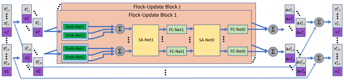
Accordingly, we propose the architecture illustrated in Fig. 1. The architecture consists of flock-update blocks, each combining two parallel sub-particle embedding networks, with permutation-invariant SA architecture. In the basic flock-update block, each state particle-weight pair is separated to single sub-state sub-particles (where the weight is shared among all sub-particles). These are transformed into two sub-particle embeddings of length , main and secondary, by two separate embedding fully connected (FC) networks, coined and , respectively. For each of the particles, each sub-particle main embedding is added to the mean of the other sub-particles secondary embeddings to get its full embeddings of the same dimension . Note that this procedure is invariant to the order of the sub-particles, thus maintaining the desired permutation invariance. Moreover, the same two embedding networks are used for all sub-particles, and thus the architecture is invariant to the number of sub-states , satisfying R4.
The full embeddings are then combined using dedicated SA blocks (e.g., in the architecture illustrated in Fig. 1, two such blocks are used). In these blocks, for each of the sub-states, all full sub-particles embeddings from all particles are updated in the same SA layer () considering all full embeddings associated with the same sub-state. This layer is followed by an FC network () applied in parallel to each of the SA outputs, thus maintaining the particle permutation invariance of the SA layer. To get each particle update, at the output of the last FC layer, the sub-states updates are concatenated while the weights are averaged. For intermediate filtering stages applications where each particle’s sub-state is assigned with its own weight, the initial weight sharing and final weight averaging can be skipped.
Inspired by multi-head attention mechanisms [36], we apply flock-update blocks in parallel. The outputs are summed up with the initial particle-weight pairs to get the final particle. On flock-update block , , prior to the last FC network, all embeddings for each sub-state are averaged, providing a single embedding per sub-state, that is turned into a single particle correction term at the final output of the block. That single particle term acts as baseline per sub-state and is added to all particles correction terms (from all other flock-update blocks), shifting their entire induced PDF accordingly.
We note that the architecture and its trainable parameters, as well as the described particles and sub-particles processing, is invariant to the number of sub-states and to their internal ordering (thus holding R4). They are also invariant to the number of particle-weight pairs and to their ordering, while enabling parallel operation (thus facilitating R3). Accordingly, the same trained architecture can be applied in settings with different numbers of sub-states and particles, e.g., an architecture trained for MTT with a small number of targets (and/or particles) can be readily applied to track a larger number of targets (and/or particles), as we show in Section IV.
III-C Loss Function
The training of tunes , encourages its correction term to satisfy two main properties: to gauge the accuracy of the state estimate (8); to align the PDF represented by a set of particles, and approximated using (7), with a desired PDF. We next formulate the proposed loss assuming supervised settings (S2), after which we show how it can be specialized to unsupervised scenarios (S1).
III-C1 Loss Formulation
The loss used for training based on data is comprised of two main parts, and , corresponding to accuracy (Property ) and heatmap representation (Property ), respectively. The resulting loss is given by
| (11) |
where and are non-negative hyperparameters balancing the contribution of each loss term.
Focusing on multiple sub-states tracking, for Property , evaluated in , we employ the optimal subpattern assignment (OSPA) measure [51], often used to represent accuracy in MTT. Specifically, we employ the OSPA distance with order of and infinite cutoff, calculated per time-step, i.e.,
| (12) |
In (12), represents the state estimation computed via (8) and the corrected set of particles on time-step .
Property is evaluated in , by comparing the distribution induced by the resulting particles with some oracle distribution. In particular, this loss term is comprised of the norms between the oracle true/desired posterior and its sub-states’ per dimension variances, denoted and , respectively, and the corresponding reconstructed values obtained from the particles, corrected using the LF block. For the latter, the reconstructed PDF, denoted , is computed via (7), while the variances term of sub-particles denoted is computed as the variances across the dimensions of the sub-particles of sub-state . The resulting loss term is given by
| (13) |
where is a hyperparameter. The PDFs comparison is performed over a set of points in the state-space, hereby referred to as the grid points, selected in one of two ways that are detailed in Subsection III-C3; and the variances comparison aims to align particles that stray too far out from the grid points region to be accounted for.
III-C2 Evaluating the Loss
Evaluating (11) requires, for each time instance , access to the true/desired state , the oracle posterior and variances . To obtain the oracle posterior and variances, we use the pertinent PF with particles, with the oracle variances attained as described for using the reference flow particles. Obtaining the oracle posterior and the true state differs based in the settings (S1 or S2):
- O1
-
O2
In the supervised settings S2, the true state is available in the data, and is isotropic multivariate Gaussian distributions centered in the true sub-states, with variances equal to the average .
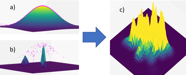
The last remaining component needed to evaluate (11) is the PDF induced by the particles and their weights, . We do that using (7) and a set of -dimensional Gaussian kernel functions we named adapting kernels illustrated in Fig. 2. These Kernel functions are set to have covariances , with determined such that all kernels have equal volume that sum up to , and with peak height of . Using these settings, particles in high probability regions (where they are likely to have other particles close by) will be assigned with high and narrow kernels, and in case that they are too close, will be encouraged to disperse by the locally lower desired PDF on the loss. Similarly, particles in low probability regions (where they are likely to be isolated) will be assigned with wide kernel functions, and so, will be encouraged by the loss to be more evenly distributed. This formulation supports adapting the grid points resolutions according to the particles predicted density, as well as boosts a smooth and accurate PDF reconstruction.
III-C3 PDF Comparison
The comparison of the two PDFs, i.e., the term in (13), is approximated by computing their differences over a grid, and the selection of the grid points highly impacts the usefulness of the loss. We present two methods for choosing the grid points around the sub-states locations:
Staged Meshgrid: The first method selects the grid points to be evenly distributed on a -dimensional cube, or a meshgrid, while adaptively tuning its scale, resolution and location. As illustrated in Fig. 3, the PDFs in (13) are compared times with different grids of the same size and different resolutions, co-centered according to and . The overlaps between the different resolutions is accounted for once on the higher resolution, that is also considered in the grid points weighting in the loss.
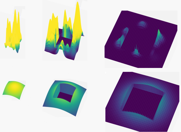
Using adapting kernels together with staged meshgrid tackles two of the main challenges encountered in PFs – sample impoverishment and particle degeneracy – as well as stochastic outliers. Sample impoverishment tends to happen close to the center of the support of the PDF, or in high resolution meshgrid stages, that can accommodate the more narrow kernels that are likely to be used there. Particle degeneracy usually occurs in the edges of the support of the PDF where the covered area is bigger and probability density is lower; there, the adapting kernels will tend to be wider and cover larger area so can be captured by the lower resolution stages. We implement and test the staged meshgrid method in Subsection IV-B.
Random Grid: Despite the aforementioned benefits of our staged meshgrid approach, it may be computationally intensive in some settings, particularly when the sub-state is of a high dimension . An alternative approach uses a random grid. Here, instead of the evenly spread points as on a meshgrid, we randomize sampling points according to a predetermined distribution. Similar to the staged meshgrid, the random grid points sampling distribution can have different density in different regions to accommodate changing resolutions and tackle particle degeneracy and sample impoverishment. Pseudo-random sampling points will result in more evenly distributed points and a better cover of the area of interest, and may induce faster and better learning, however this is left for future work. The random grid method is numerically evaluated in Subsection IV-A.
III-D Training
We note that the loss function in (11) expresses a sum of time-steps components of (12), and (13), computed separately at each time-step when an LF block with parameters is applied. We can leverage this property to enable training LF on each (or selected) time-step seperately using conventional stochastic gradient descent (SGD)-based learning, while avoiding the need for differentiability between iterations (and avoiding the need to backpropagate through sampling operators using special sampling adaptations [52, 53], or by introducing approximated operators [29, 28]).
A candidate training method based on mini-batch SGD for an LF-PF is formulated in Algorithm 3. There, the LF-PF is executed in parallel with the reference PF flow (Steps 3, 3), that maintain particles-weights sets for each trajectory, respectively denoted for the th time step of the th batch. Training is done by loss calculation (Steps 3-3) and its backpropagation (Step 3), while nullifying gradient propagation between iterations and through sampling operations. To achieve a fast and continuous convergence, on each time-step we mix the loss of different trajectories by running a bigger batch of trajectories , while training on a random subset of the batch that changes between time-steps (Step 3). For tracking stabilization during training, particularly at the beginning, once an estimated sub-state strays farther than a predetermined distance from the desired sub-state (Step 3) the whole trajectory is eliminated from for the training on the following time-steps (Step 3).
III-E Discussion
The proposed trainable LF module is trained as part of a specific PF, and possibly with an additional more complex PF serving as reference. Nonetheless, once trained, it can be readily transferred into alternative PFs that meet R1, as demonstrated in Subsection IV-A. Moreover, by harnessing supervised data, the LF-PF can also cope with R2 without incorporating additional mechanisms to explicitly mitigate it as in [54]; while enabling the pertinent PF to operate with a smaller number of particles with minimal computational cost to meet R3. As discussed in Subsection III-B, the LF architecture is invariant to the number of sub-states , and, e.g., the same module can be trained and evaluated for tracking a different number of sub-states, thus meeting R4. These properties are consistently demonstrated in Subsection IV-B.
Our LF module, trained with a specific number of particles, allows PFs to operate reliably with different, and even lower values of , boosting low latency filtering. However, the application of LF comes at the cost of some excessive complexity, depending on the parameters , , , , , as well as the flock-update parameters, number of sub-embeddings (, or to include secondary embedding), number of SA blocks , and FC width multiplier . The total floating point multiplications (FPM) requirement per particle can be divided to three parts with accordance to Fig. 1: broadly speaking, the embedding networks require FPM; the SA networks involve ; and the final FC layers require FPM. While this excessive complexity varies considerably with the system parameters, it is noted that the operation of such compact DNNs is highly suitable for parallelization and hardware acceleration, that often notably reduces inference speed of PFs with similar performance, as demonstrated in Section IV.
Our proposed LF jointly corrects particles and their weights utilizing only the particles and weights (that are merely updated by the LF block). This boosts versatility and flexibility enabling a trained LF block to be conveniently integrated and apply a fix to a flock at any point on different types of PFs flow, whether classical or DNN augmented, or even to a different PF than the one it was trained on (as shown in Subsection IV-A). Nonetheless, one can potentially extend LF to process additional information when updating the particles, such as past particles (smoothing), the measurements, and data structures [55]. Moreover, the LF block can be adapted to change its output, for instance, to include an estimated state or additional embedding for other purposes. It can possibly also be integrated in PFs involving detection (e.g., track-before-detect [7]). We leave these extensions for future work.
IV Experimental Study
In this section, we numerically evaluate our LF algorithm in terms of performance and latency. We first compare it to state-of-the-art PF neural augmentation for synthetic state estimation in Subsection IV-A. Then, in Subsection IV-B we combine our LF with a well-established APF for a radar MTT setup111The source code and hyperparameters used in this experimental study is available at https://github.com/itainuri/LF-PF_MTT.git.. All timing/latency tests were computed on the same processor, AMD EPYC 7343 16-Core 3.2GHz.
IV-A Synthetic State Estimation
Here, we evaluate LF-PF in comparison to state-of-the-art neural augmentation of PFs, based on algorithm unrolling [31]. Our goal here is to showcase the performance gains of our proposed LF algorithm compared to alternative types of DNN augmentations, and that its operation is complementary to other enhancements of PFs.
IV-A1 Simulation Setup
We adopt the synthetic simulation setup used in [31]. Here, the state is comprised of dimensional variables, and is tracked based on observations of dimension over time-steps. The state evolution model is given by
| (14) |
while the observation model is
| (15) |
In (14)-(15), and are fixed matrices taken from [31, Ch. 4.1] and the noise vectors and are zero-mean with covariances and , respectively. Specifically, the noise distributions and the mapping are taken from the following setups:
-
X1
A linear Gaussian system, where and and are zero-mean white Gaussian noises with fixed covariance matrices and taken from [31, Ch. 4.1].
-
X2
Gaussian noise as in X1, with non-linear given by the absolute value function (taken element-wise).
-
X3
A non-Gaussian system, where , with non-Gaussian uniform noise and mismatched assumed covariance matrices and .
The noise covariances have the same norm, i.e., , dictating the signal-to-noise ratio (SNR).
IV-A2 Estimation Algorithms
Our main baseline PF throughout this section is the SISPF [16]. This estimator implements Algorithm 1 with a Gaussian sampling distribution , whose inverse covariance is , and mean is .
Based on the formulation of the SISPF to the above models, we compare the following estimation algorithms:
-
•
SISPF with and with particles.
-
•
An augmented (LF-SISPF) with particles. With dictated by the settings, and with , , , and , the LF module has trainable parameters , and FPM per particle per iteration with particles. The reference PF used for training an is SISPF with particles, with the heatmap loss PDFs in (13) compared over random grid points with Gaussian distribution.
-
•
The UrPF of [31], which unrolls PF time-steps. All steps use the same covariance DNN and each step uses a dedicated mean DNN for a multivariate normal importance sampling function. The DNNs receive a particle and the measurements as input, and have learnable parameters , and require FPM per particle per particles iteration.
-
•
augmented (LF-UrPF), Augmenting the trained data-based UrPF with an LF module, trained with the model-based SISPF (both with the same and ).
All data-driven estimators were trained in an unsupervised manner: LF-SISPF via O1, and UrPF as described in [31]. We use the mean-squared error (MSE) as our performance measure, evaluated over a test trajectories, a times each. For each scenario we trained the LF-SISPF model on long trajectories, keeping the best weights according to time-step , and considering time-steps for the loss. For each setup, training was initially done with SNR=0 dB and fine-tuned for each SNR. While the same LF pre-trained weights were applied on all trajectories of the same experiment, the UrPF was trained per test trajectory (per experiment). Specifically, we trained UrPF for epochs on that time-steps trajectory without resampling, keeping the best weights for testing according to two criteria, for the full trajectory average, and for the last time-step average.
IV-A3 Results
We test each of the benchmarks in all three settings with different SNRs. All benchmarks have particles resampling procedure cooperated to their iteration flow, and testing is performed twice, once with and once with (without resampling). For clarity considerations we chose to present the experiment with the better results out of the two, where the SISPF with particles was always implemented with resampling.
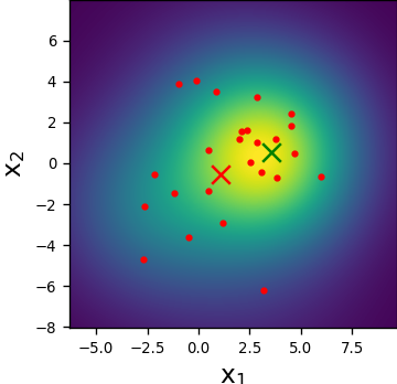
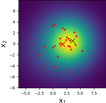
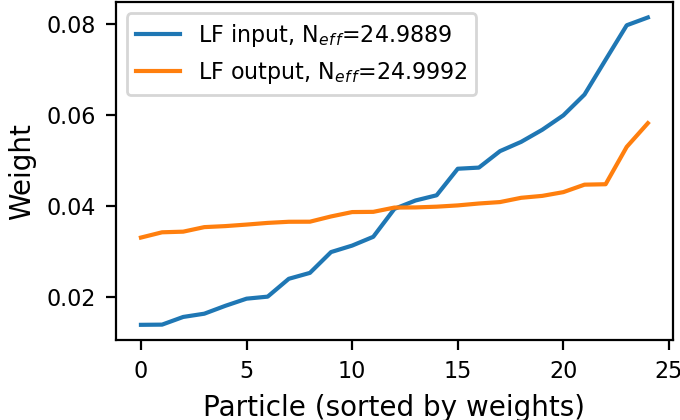
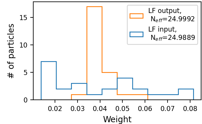
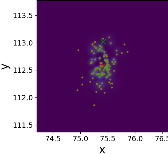
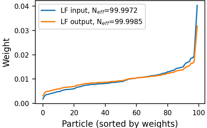
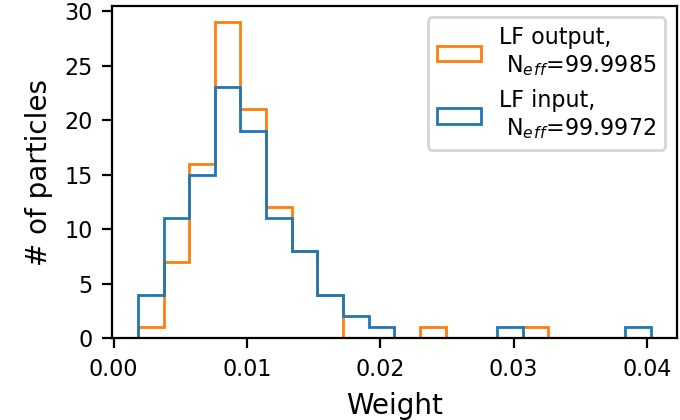
We first visualize the ability of the LF module in forming desirable particle patterns. To that aim, we observe the operation of a trained LF module for the settings X3 at a given time instance and SNR of dB. We illustrate in Figs. 4(a)-4(b) how the trained LF block herds the particles closer to the desired location (on and axes), and how the new induced PDF is more confined and the estimation is more accurate. We also examine the weights at the input and output of our LF block in Figs. 4(c)-4(d). There, we observe a reduction in the variance of the weights and an increase in the effective number of particles (without explicitly encouraging it via the loss), which potentially indicate an improved capture of the PDF. This constant correction of the particles and weights alleviates the degeneracy phenomenon, as can be seen by the initial high on time-step .
We next show that the favourable particles and weights alternations achieved by LF on a single time-step, as presented in Fig. 4, translate into improved tracking accuracy. To that aim, we report in the Fig. 5 the resulting OSPA values achieved by the considered tracking algorithms for settings X1-X3 in recovering the entire trajectory (Figs. 5(a)-5(c)) and in recovering solely the final time-step (Figs. 5(d)-5(f)), being the task for which UrPF is originally designed for, in [31].
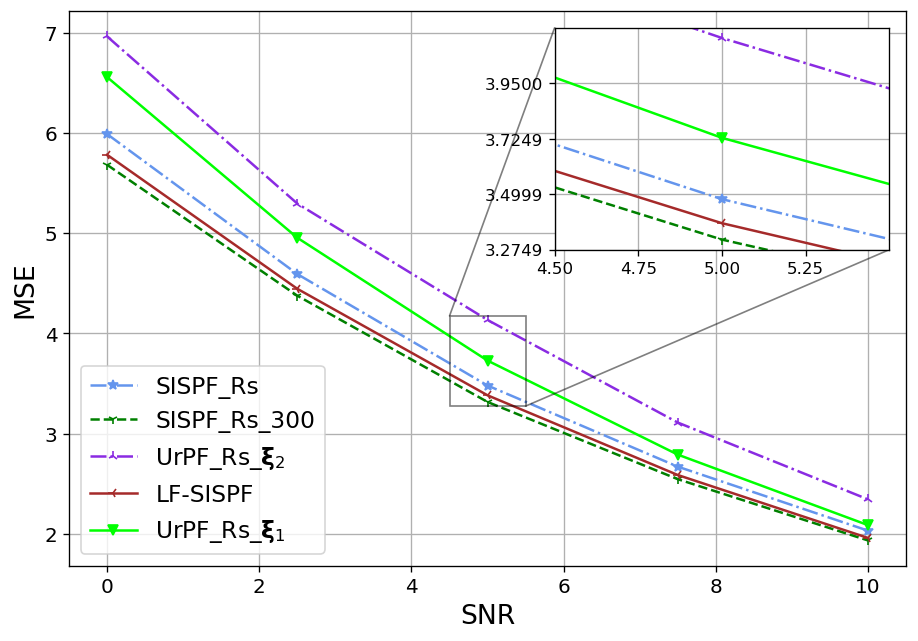
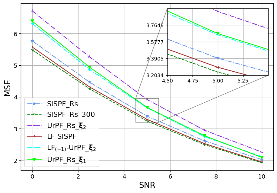
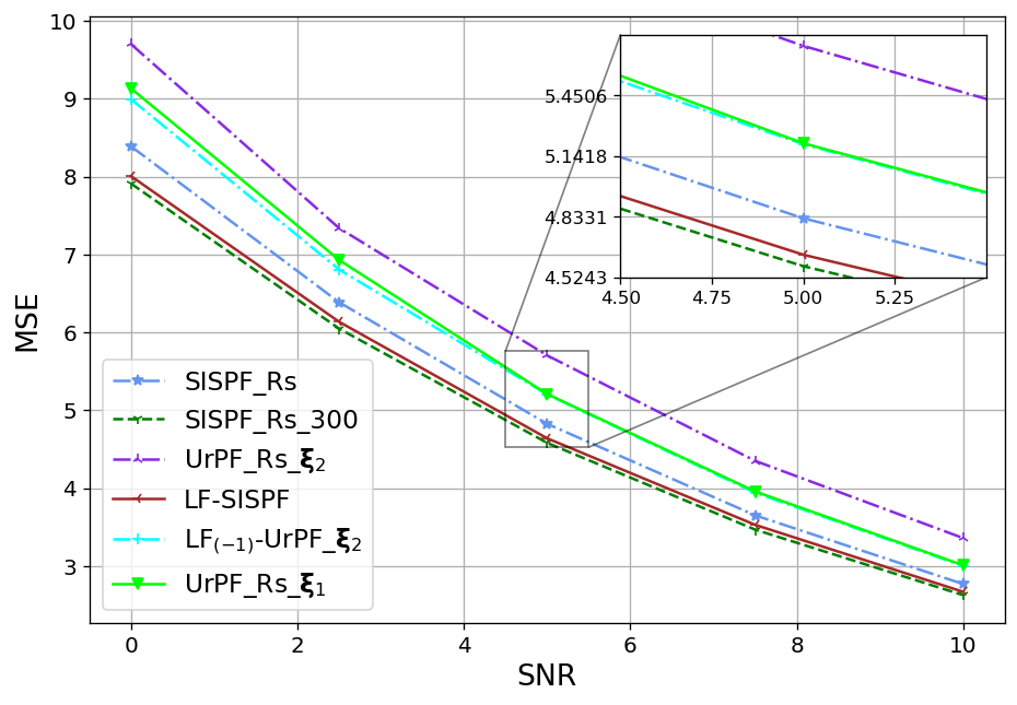
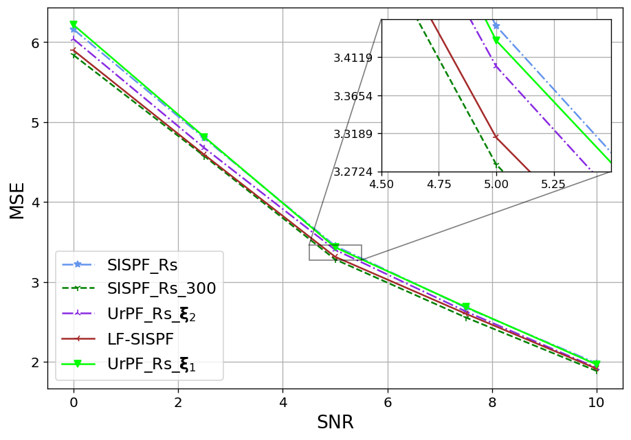
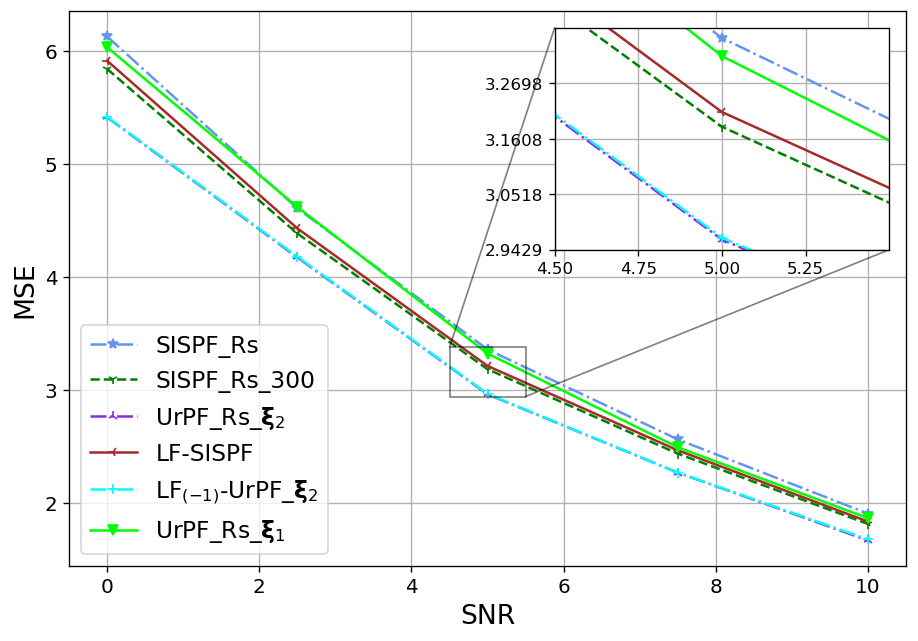
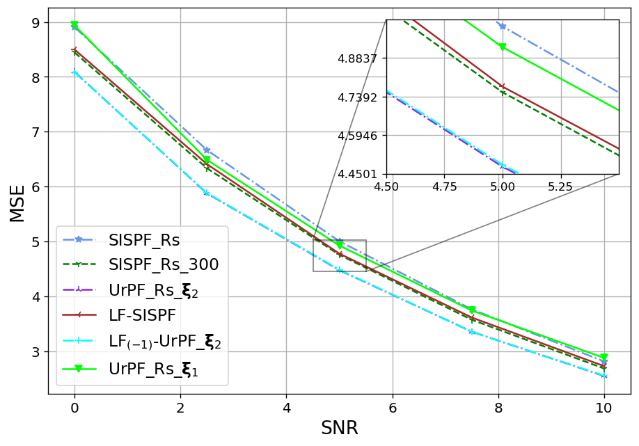
As observed in Fig. 5, on all experiments the LF-SISPF notably improves the SISPF and achieves results that are close to those of its teacher PF, namely, the SISPF with . In the straightforward X1 settings our LF-SISPF accuracy surpasses that of the UrPF in all experiments (Figs. 5(a) and 5(d)), while operating with a similar number of FPM and with a number of trainable parameters that is independent of trajectory length, and without considering the measurements. On the more complex X2 (Figs. 5(b) and 5(e)) and X3 (Figs. 5(c) and 5(f)) cases, LF outperforms the overall accuracy of the UrPF (Figs. 5(b) and 5(c)), but outperformed by it on the last time-step criterion (Figs. 5(e) and 5(f)). This can be attributed to the inferiority of the reference PF used in training, i.e., , as well as to the specialized training of the UrPF, that is trained separately for each specific trajectory and each specific task. This specialization may be the cause of the deteriorated accuracy of the UrPF on one task when trained for the other ( on the top sub-figures and on the bottom sub-figures).
The LF-UrPF experiments demonstrate the versatility of our algorithm, incorporating our LF module to the DNN augmented UrPF on selected time-steps. Even though the LF module was trained to improve another (classical) PF, its augmentation to the has improved it and the accuracy on Figs. 5(b) and 5(c) surpasses those of on the overall accuracy while maintaining accuracy on the last time-step on Figs. 5(e) and 5(f). Moreover, while the LF module comes at the cost of some excessive complexity, as analyzed in Subsection III-E, its gains in performance greatly outweigh its additional induced latency that is reported in Table I. The runtime values, reported in Table I, together with Fig. 5, showcase the advantages of LF, in allowing to notably enhance performance with limited particles without significantly increasing inference latency.
| SISPF | SISPF | LF-SISPF | UrPF | LF-UrPF | |
|---|---|---|---|---|---|
| 300 | 25 | 25 | 25 | 25 | |
| mS | 335.499 | 31.323 | 72.183 | 177.197 | 213.320 |
IV-B Radar Target Tracking
We proceed to evaluating LF-PF for non-linear radar tracking, considering both a single and multiple targets. We use the non-linear settings outlined in [7, Sec. VI], which allow us to compare the performance and latency of PFs to their LF augmented versions in a scenario of practical importance.
IV-B1 Experimental Setup
In the considered scenarios, which are based on [7, Sec. VI], the state represents the positions and velocities of a fixed number of targets in two-dimensional space over trajectories of length , with up to targets. Each target is independent of other targets and follows 14 with and and taken from [7, Sec. VI.A]. The measurements capture a sensor response solely to the targets’ locations, following the sensor model of [7, Sec. VI.A]. We consider three different settings:
-
Y1
Single target in calibrated settings, tracking with sensors located meters apart on meters 2-dimensional plane, with different SNRs.
-
Y2
Single target in mismatched settings, same assumed model where the actual sensors locations are perturbed with random Gaussian noise, with different SNRs.
-
Y3
MTT of targets, a single SNR, calibrated settings.
IV-B2 Estimation Algorithms
Similar to Algorithm 2, we augment the APP, a version of the APF proposed in [7], prior to its integrated Kalman filter that tracks the target velocity. Accordingly, we compare the following PFs:
-
•
APP from [7] with single and multiple target support.
-
•
augmented (LF-APP) for single target. LF module with , , ; while (for calibrated settings) and (for mismatched settings).
-
•
MTT LF-APP, with LF module with , , , , and .
All LF-APP benchmarks were trained according to Algorithm 3, via O1 in the calibrated settings and via O2 in the mismatched settings. All training was done on a single SNR using particles and with batches and sub-batches sizes between and . Training, validation and testing performances are the average OSPA [51] metric (assigned per time-step), evaluated over all time-steps, with cutoff of (and infinite cutoff on training) and order of (see [51] for details). The heatmap loss was computed using staged meshgrid with and (on Y1,Y2) and (on Y3) grid points. For all settings, we randomly combine a set of single target sub-trajectories for training and two such sets of , for validation and testing.
IV-B3 Results
we divide our results into three parts with respect to Y1-Y3 and compare the benchmarks for accuracy, performance, and latency, with accuracy results averaged over trajectories. We visualize a single target trajectory tracking on Y2 as well as an MTT one in Y3 settings with targets. As in Subsection IV-A, we also visualize the ability of LF to enhance the particles and weights and their associated reconstructed PDF on a single time-step on MTT with .
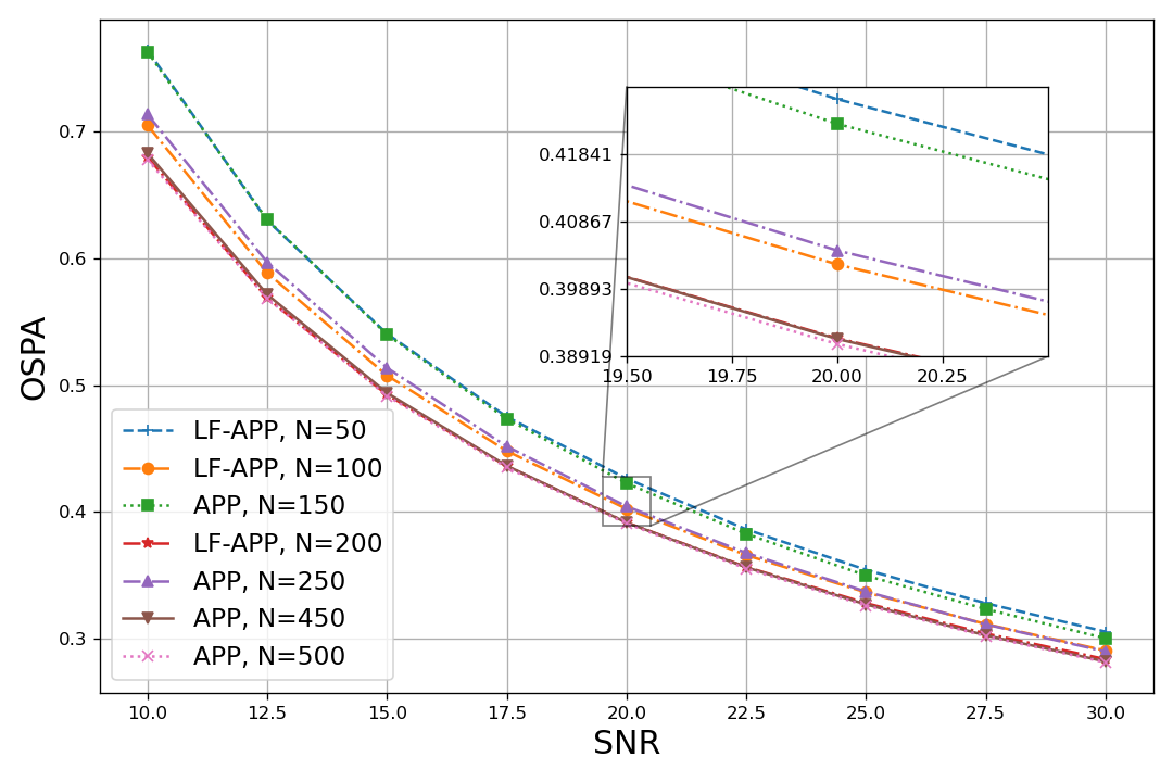
Single target in calibrated settings (Y1): We first compare the accuracy achieved by the APP to that of the LF-APP, trained on . The resulting OSPA versus SNR, reported in Fig. 6, demonstrate that, although trained with particles and a single SNR, the correction term added by our LF block allows APP to systematically achieve performance equivalent to times more particles on a wide rage of SNRs. We also note that the improvement, induced by our Algorithm is more significant on lower SNRs.
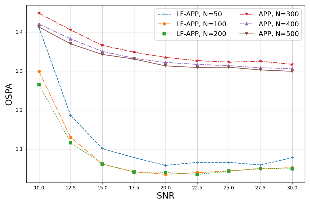
Single target in mismatched settings (Y2): For the mismatched case, we employ LF-APP with , trained on . The results, reported in Fig. 7 show that LF-APP notably improves performance with similar consistent improvement with increased , but also yields an error floor for the model-based APP. To show that this gain is directly translated into improved tracking, we illustrate in Fig. 8 the tracking of a single sub-state trajectory, where the LF augmentation is shown to notably improve tracking accuracy.
We proceed by evaluating the excessive latency of LF-APP. We report in Table II the latency of both APP and LF-APP used for both experiments in milliseconds. The timing results in Table II indicate that while latency grows dramatically with , the excessive latency induced by incorporating our LF block is minor. Combining this with Figs. 6 and 7 showcases the ability of LF-APP in allowing PFs (such as the APP) to meet R1-R3 on a wide range of single target scenarios.
| APP | LF-APP, | LF-APP, | |
|---|---|---|---|
| 50 | 8.200 | 11.548 | 14.039 |
| 100 | 13.993 | 19.400 | 20.828 |
| 200 | 34.147 | 36.177 | 38.082 |
| 300 | 50.221 | 53.046 | 55.666 |
| 400 | 66.195 | 69.797 | 73.393 |
| 500 | 81.986 | 86.749 | 91.245 |
MTT in calibrated settings (Y3): We proceed to compare the APP and the LF-APP for their accuracy, performance and latency for a known and fixed number of targets , taking values between and and with different numbers of particles . Training was done by jointly learning [56] on data corresponding to , , (with equal probability) and (10% of trajectories) targets tracking scenarios with , and with validation on targets tracking. Since the basic form of our LF tested here has a per time-step operation, and in order to isolate its evaluation, we address training and testing in the same manner, and the mapping between estimations and true targets is done separately on each time-step according to the best OSPA, effectively disregarding target swaps between time-steps.
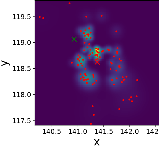
Fig. 9 illustrates the operation of our LF block on a single frame three target tracking on time-step . Figs. 9(a)-9(f) visualize its improving of the spread of the three sets of sub-particles by dispersing clusters and reducing outliers. Figs. 9(g)-9(h) show that our trained LF module encourages low variance of the weights without explicitly doing so in the loss, implying a better utilization of the particles. We again observe that is close to already at the input of our LF module, hinting the effectiveness of our LF algorithm in describing the PDF along the whole trajectory, as well as strengthens its effectiveness [57], as it is useful also for enhancing in settings where .
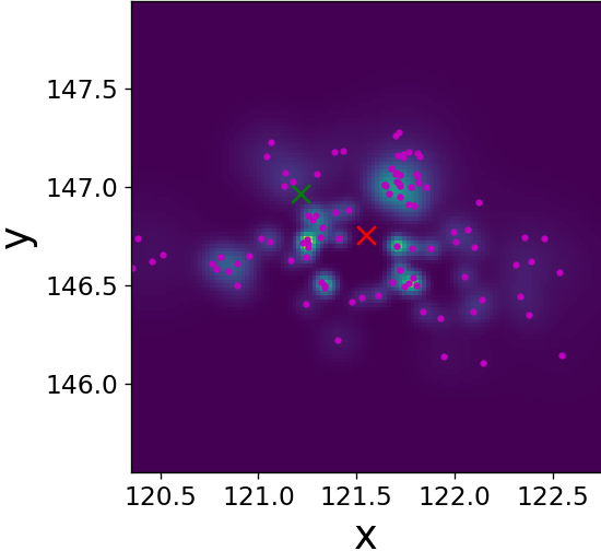
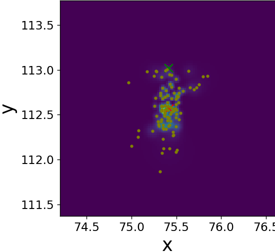
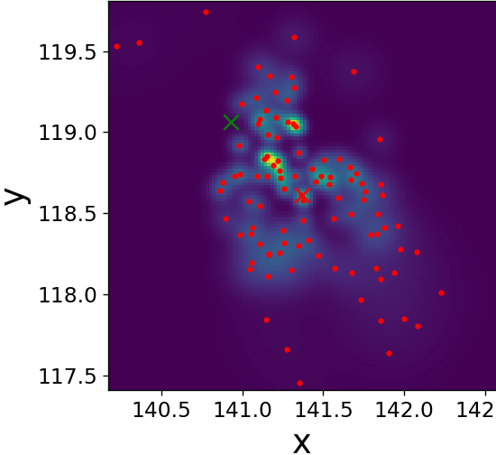
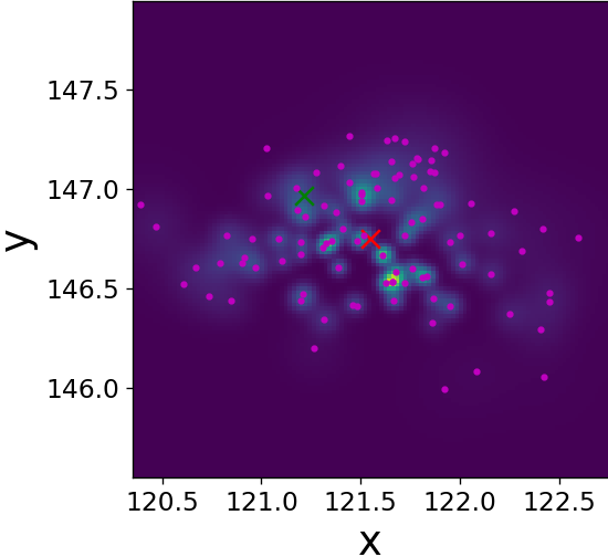
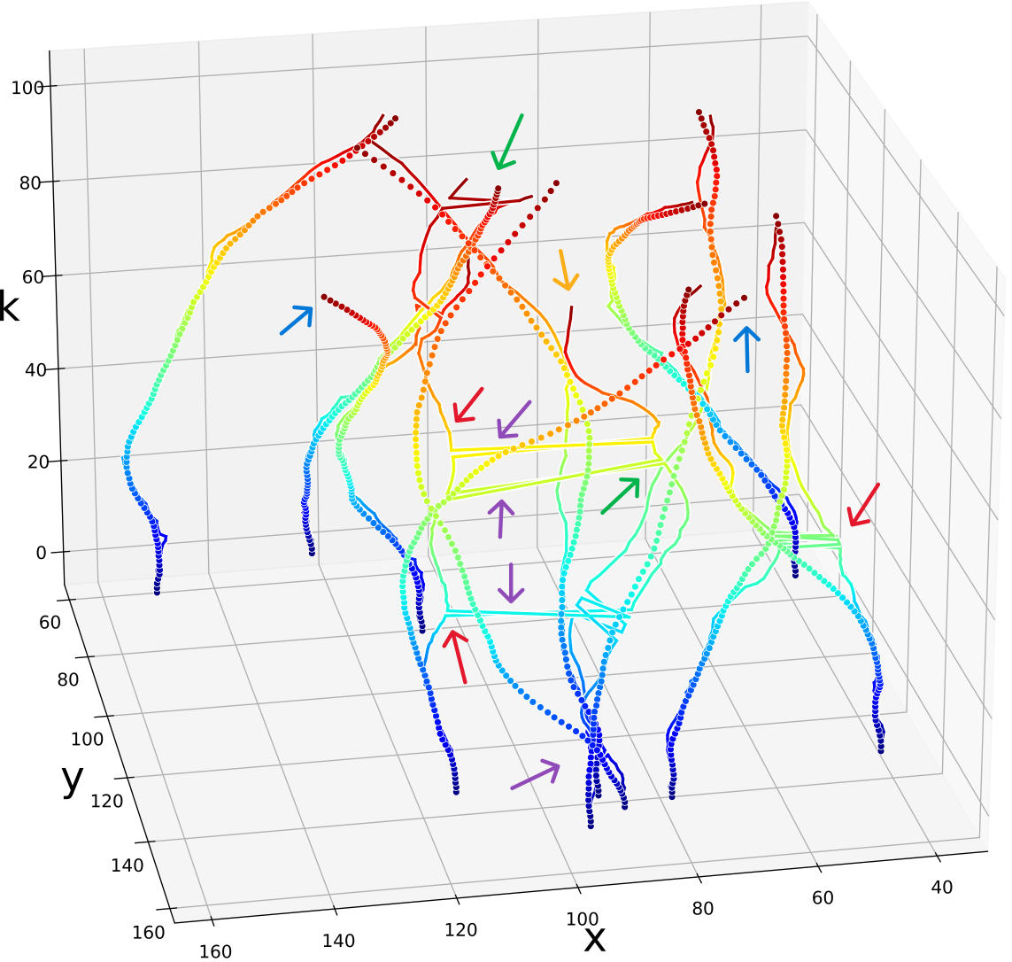
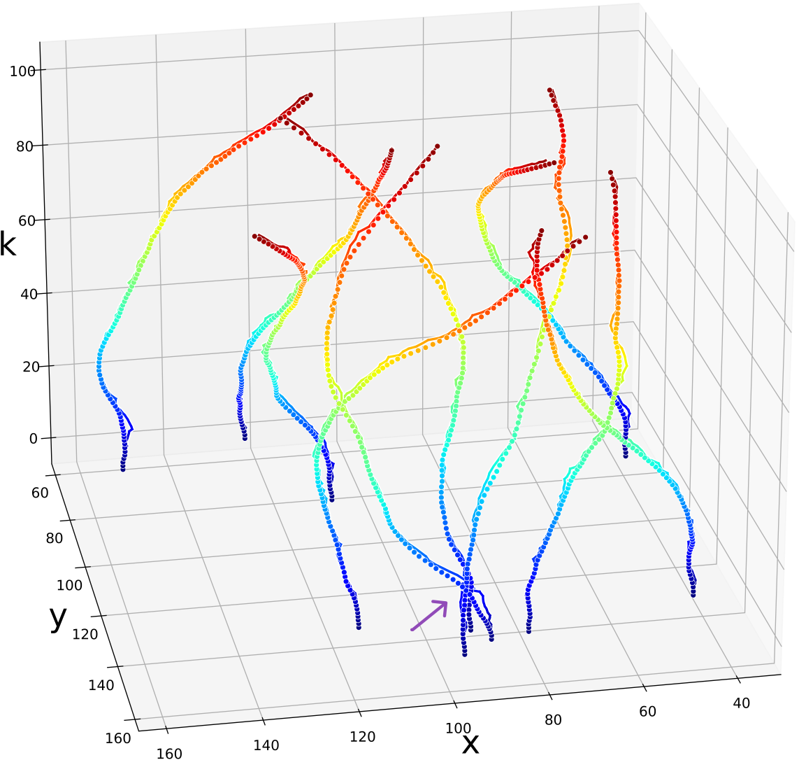
Single time-step improvements on the spread of the sub-particles as presented on Fig. 9, applied to each time-step, have a major effect on the overall tracking of the targets along the full state trajectory. Fig. 10 illustrates this benefit on a target MTT simulation. There, we can see the improvement in terms of a diminished number of lost targets, better targets-estimations mapping injectiveness and better accuracy. Further, even though we did not explicitly encourage it in our loss function, we also witness less targets-estimations mapping swaps. Examples of the aforementioned improvements are highlighted on Fig. 10 with arrows of respective colors.
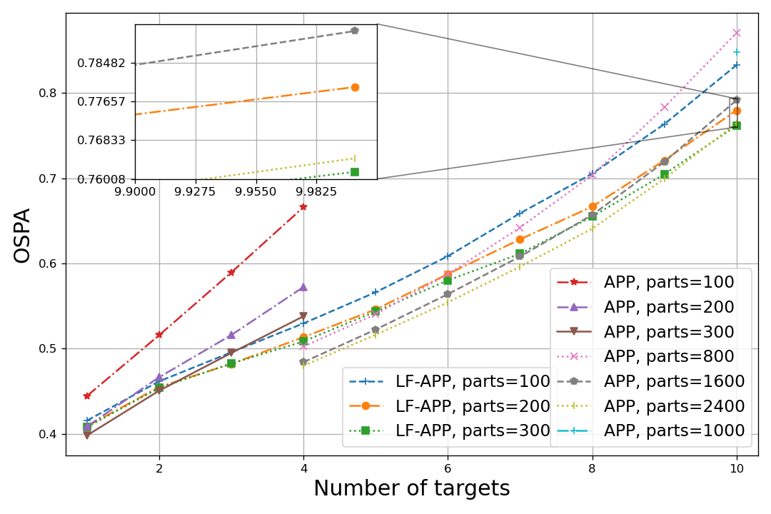
The translation of these improvements into tracking accuracy is showcased on Fig. 11. rained with particles and applied with varying number of particles, Fig. 11 illustrates that LF provides greater improvement in performance as the number of targets increases. While trained with up to targets on only of the trajectories, LF achieves a significant reduction in the required number of particles when handling targets, consistently reducing it by a notable factor of , and up to with a particles.
Complementary to Fig. 11, Table III compares the tracking latency of the APP and LF-APP with different numbers of particles and targets. Combining the results in Fig. 11 and Table III, and comparing them to the Y1 results in Fig. 6 and Table II, consistently demonstrate that the benefit of our LF algorithm in coping with the challenging task of tracking multiple targets with limited latency is more prominent and potentially more beneficial than in single target settings.
| 1 | 2 | 4 | 6 | 8 | 10 | ||
|---|---|---|---|---|---|---|---|
| 100 | APP | 14.62 | 28.24 | 49.34 | 73.32 | 101.393 | 135.10 |
| LF-APP | 24.08 | 41.33 | 66.24 | 98.32 | 135.52 | 172.35 | |
| 200 | APP | 35.52 | 53.89 | 95.29 | 142.35 | 198.011 | 260.86 |
| LF-APP | 44.66 | 79.95 | 127.64 | 189.11 | 263.19 | 337.53 | |
| 300 | APP | 52.12 | 79.51 | 141.14 | 211.19 | 295.751 | 386.41 |
| LF-APP | 64.94 | 116.26 | 189.63 | 288.43 | 391.55 | 505.67 | |
| 800 | APP | 129.93 | 203.29 | 362.40 | 542.73 | 803.78 | 999.30 |
| 1600 | APP | 257.77 | 404.08 | 720.87 | 1087.01 | 1624.70 | 1996.31 |
| 2400 | APP | 385.63 | 595.86 | 1046.25 | 1569.93 | 2184.01 | 2824.22 |
V Conclusions
We introduced a neural augmentation of PFs using a novel concept of LF, that supports changing numbers of sub-states and particles. LF is designed to enhance state estimation by adjusting a PF’s particles at any point in its flow, solely based on the interplay between the particles, resulting in an improved output. We realize LF using a dedicated DNN architecture that accounts for the permutation equivariance property of the particle-weight pairs in PFs, and introduce a dedicated training framework that supports both supervised and unsupervised learning, while accommodating high-dimensional sub-state tracking and with indifference to the particles acquirement procedure. Once trained, the LF module is easily transferable to most PFs, and can even be combined with alternative DNN PF augmentations. We experimentally exemplified the gains of LF in terms of performance, latency, and robustness and even in overcoming mismatched modelling, demonstrating its potential for enhancing variety of PFs and as a foundation for enhancement of more intricate PF filtering tasks.
References
- [1] I. Nuri and N. Shlezinger, “Neural augmented particle filtering with learning flock of particles,” in IEEE International Workshop on Signal Processing Advances in Wireless Communication (SPAWC), 2024.
- [2] P. M. Djuric, J. H. Kotecha, J. Zhang, Y. Huang, T. Ghirmai, M. F. Bugallo, and J. Miguez, “Particle filtering,” IEEE Signal Process. Mag., vol. 20, no. 5, pp. 19–38, 2003.
- [3] S. Thrun, “Particle filters in robotics.” in Uncertainty in AI (UAI), vol. 2. Citeseer, 2002, pp. 511–518.
- [4] P. Djurić, J. Zhang, T. Ghirmai, Y. Huang, and J. H. Kotecha, “Applications of particle filtering to communications: A review,” in 2002 11th European Signal Processing Conference. IEEE, 2002, pp. 1–4.
- [5] F. Gustafsson, F. Gunnarsson, N. Bergman, U. Forssell, J. Jansson, R. Karlsson, and P.-J. Nordlund, “Particle filters for positioning, navigation, and tracking,” IEEE Trans. Signal Process., vol. 50, no. 2, pp. 425–437, 2002.
- [6] Y. Boers and J. Driessen, “Multitarget particle filter track before detect application,” IEE Proceedings-Radar, Sonar and Navigation, vol. 151, no. 6, pp. 351–357, 2004.
- [7] L. Ubeda-Medina, A. F. Garcia-Fernandez, and J. Grajal, “Adaptive auxiliary particle filter for track-before-detect with multiple targets,” IEEE Trans. Aerosp. Electron. Syst., vol. 53, no. 5, pp. 2317–2330, 2017.
- [8] N. Ito and S. Godsill, “A multi-target track-before-detect particle filter using superpositional data in non-Gaussian noise,” IEEE Signal Process. Lett., vol. 27, pp. 1075–1079, 2020.
- [9] J. Durbin and S. J. Koopman, Time series analysis by state space methods. Oxford University Press, 2012.
- [10] S. Buzzi, M. Lops, and L. Venturino, “Track-before-detect procedures for early detection of moving target from airborne radars,” IEEE Trans. Aerosp. Electron. Syst., vol. 41, no. 3, pp. 937–954, 2005.
- [11] G. Grisetti, C. Stachniss, and W. Burgard, “Improving grid-based slam with Rao-Blackwellized particle filters by adaptive proposals and selective resampling,” in IEEE international conference on robotics and automation, 2005, pp. 2432–2437.
- [12] P. Closas and C. Fernández-Prades, “Particle filtering with adaptive number of particles,” in IEEE Aerospace Conference, 2011.
- [13] D. Xu, C. Shen, and F. Shen, “A robust particle filtering algorithm with non-gaussian measurement noise using student-t distribution,” IEEE Signal Process. Lett., vol. 21, no. 1, pp. 30–34, 2013.
- [14] A. T. Fisch, I. A. Eckley, and P. Fearnhead, “Innovative and additive outlier robust kalman filtering with a robust particle filter,” IEEE Trans. Signal Process., vol. 70, pp. 47–56, 2021.
- [15] T. Li, M. Bolic, and P. M. Djuric, “Resampling methods for particle filtering: classification, implementation, and strategies,” IEEE Signal Process. Mag., vol. 32, no. 3, pp. 70–86, 2015.
- [16] A. Doucet, S. Godsill, and C. Andrieu, “On sequential monte carlo sampling methods for bayesian filtering,” Statistics and computing, vol. 10, pp. 197–208, 2000.
- [17] M. Piavanini, L. Barbieri, M. Brambilla, and M. Nicoli, “Annealed Stein particle filter for mobile positioning in indoor environments,” in IEEE International Conference on Communications (ICC), 2023, pp. 2510–2515.
- [18] I. Goodfellow, Y. Bengio, and A. Courville, Deep Learning. MIT Press, 2016, http://www.deeplearningbook.org.
- [19] N. Shlezinger, J. Whang, Y. C. Eldar, and A. G. Dimakis, “Model-based deep learning,” Proc. IEEE, vol. 111, no. 5, pp. 465–499, 2023.
- [20] N. Shlezinger, Y. C. Eldar, and S. P. Boyd, “Model-based deep learning: On the intersection of deep learning and optimization,” IEEE Access, vol. 10, pp. 115 384–115 398, 2022.
- [21] N. Shlezinger and Y. C. Eldar, “Model-based deep learning,” Foundations and Trends® in Signal Processing, vol. 17, no. 4, pp. 291–416, 2023.
- [22] G. Revach, N. Shlezinger, X. Ni, A. L. Escoriza, R. J. Van Sloun, and Y. C. Eldar, “KalmanNet: Neural network aided Kalman filtering for partially known dynamics,” IEEE Trans. Signal Process., vol. 70, pp. 1532–1547, 2022.
- [23] G. Revach, N. Shlezinger, T. Locher, X. Ni, R. J. van Sloun, and Y. C. Eldar, “Unsupervised learned kalman filtering,” in European Signal Processing Conference (EUSIPCO), 2022, pp. 1571–1575.
- [24] I. Buchnik, G. Revach, D. Steger, R. J. Van Sloun, T. Routtenberg, and N. Shlezinger, “Latent-KalmanNet: Learned Kalman filtering for tracking from high-dimensional signals,” IEEE Trans. Signal Process., vol. 72, pp. 352–367, 2023.
- [25] A. Ghosh, A. Honoré, and S. Chatterjee, “DANSE: Data-driven non-linear state estimation of model-free process in unsupervised learning setup,” IEEE Trans. Signal Process., vol. 72, pp. 1824–1838, 2024.
- [26] G. Revach, X. Ni, N. Shlezinger, R. J. van Sloun, and Y. C. Eldar, “RTSNet: Learning to smooth in partially known state-space models,” IEEE Trans. Signal Process., vol. 71, pp. 4441–4456, 2023.
- [27] G. Choi, J. Park, N. Shlezinger, Y. C. Eldar, and N. Lee, “Split-KalmanNet: A robust model-based deep learning approach for state estimation,” IEEE Trans. Veh. Technol., vol. 72, no. 9, pp. 12 326–12 331, 2023.
- [28] X. Chen, H. Wen, and Y. Li, “Differentiable particle filters through conditional normalizing flow,” in IEEE International Conference on Information Fusion (FUSION), 2021.
- [29] R. Jonschkowski, D. Rastogi, and O. Brock, “Differentiable particle filters: End-to-end learning with algorithmic priors,” arXiv preprint arXiv:1805.11122, 2018.
- [30] X. Ma, P. Karkus, D. Hsu, and W. S. Lee, “Particle filter recurrent neural networks,” in AAAI Conference on Artificial Intelligence, vol. 34, no. 04, 2020, pp. 5101–5108.
- [31] F. Gama, N. Zilberstein, R. G. Baraniuk, and S. Segarra, “Unrolling particles: Unsupervised learning of sampling distributions,” in IEEE International Conference on Acoustics, Speech and Signal Processing (ICASSP), 2022, pp. 5498–5502.
- [32] F. Gama, N. Zilberstein, M. Sevilla, R. G. Baraniuk, and S. Segarra, “Unsupervised learning of sampling distributions for particle filters,” IEEE Trans. Signal Process., vol. 71, pp. 3852–3866, 2023.
- [33] B. Cox, S. Pérez-Vieites, N. Zilberstein, M. Sevilla, S. Segarra, and V. Elvira, “End-to-end learning of Gaussian mixture proposals using differentiable particle filters and neural networks,” in IEEE International Conference on Acoustics, Speech and Signal Processing (ICASSP), 2024, pp. 9701–9705.
- [34] M. Piavanini, L. Barbieri, M. Brambilla, and M. Nicoli, “Deep unfolded annealed stein particle filter for vehicle tracking,” in IEEE International Conference on Acoustics, Speech and Signal Processing (ICASSP), 2024, pp. 13 226–13 230.
- [35] Y. Xia, S. Qu, S. Goudos, Y. Bai, and S. Wan, “Multi-object tracking by mutual supervision of cnn and particle filter,” Personal and Ubiquitous Computing, pp. 1–10, 2021.
- [36] A. Vaswani, N. Shazeer, N. Parmar, J. Uszkoreit, L. Jones, A. N. Gomez, Ł. Kaiser, and I. Polosukhin, “Attention is all you need,” Advances in neural information processing systems, vol. 30, 2017.
- [37] N. Shlezinger and T. Routtenberg, “Discriminative and generative learning for linear estimation of random signals [lecture notes],” IEEE Signal Process. Mag., vol. 40, no. 6, pp. 75–82, 2023.
- [38] J. Gou, B. Yu, S. J. Maybank, and D. Tao, “Knowledge distillation: A survey,” International Journal of Computer Vision, vol. 129, pp. 1789–1819, 2021.
- [39] M. K. Pitt and N. Shephard, “Filtering via simulation: Auxiliary particle filters,” Journal of the American statistical association, vol. 94, no. 446, pp. 590–599, 1999.
- [40] B.-n. Vo, M. Mallick, Y. Bar-Shalom, S. Coraluppi, R. Osborne, R. Mahler, and B.-t. Vo, “Multitarget tracking,” Wiley encyclopedia of electrical and electronics engineering, no. 2015, 2015.
- [41] N. Bergman, A. Doucet, and N. Gordon, “Optimal estimation and cramér-rao bounds for partial non-gaussian state space models,” Annals of the Institute of Statistical Mathematics, vol. 53, pp. 97–112, 2001.
- [42] M. S. Arulampalam, S. Maskell, N. Gordon, and T. Clapp, “A tutorial on particle filters for online nonlinear/non-Gaussian Bayesian tracking,” IEEE Trans. Signal Process., vol. 50, no. 2, pp. 174–188, 2002.
- [43] N. Bergman, “Recursive bayesian estimation: Navigation and tracking applications,” Ph.D. dissertation, Linköping University, 1999.
- [44] P. Rebeschini and R. Van Handel, “Can local particle filters beat the curse of dimensionality?” Ann. Appl. Probab., vol. 25, no. 5, pp. 2809–2866, 2015.
- [45] O. Straka and M. Ŝimandl, “A survey of sample size adaptation techniques for particle filters,” IFAC Proceedings Volumes, vol. 42, no. 10, pp. 1358–1363, 2009.
- [46] P. D. Moral, “Nonlinear filtering: Interacting particle resolution,” Comptes Rendus de l’Academie des Sciences-Serie I-Mathematique, vol. 325, no. 6, pp. 653–658, 1997.
- [47] P. Del Moral and L. Miclo, Branching and interacting particle systems approximations of Feynman-Kac formulae with applications to non-linear filtering. Springer, 2000.
- [48] C. Musso, N. Oudjane, and F. Le Gland, “Improving regularised particle filters,” in Sequential Monte Carlo methods in practice. Springer, 2001, pp. 247–271.
- [49] P. Bunch and S. Godsill, “Particle filtering with progressive Gaussian approximations to the optimal importance density,” in IEEE International Workshop on Computational Advances in Multi-Sensor Adaptive Processing (CAMSAP), 2013, pp. 360–363.
- [50] J. Kronander and T. B. Schön, “Robust auxiliary particle filters using multiple importance sampling,” in IEEE Workshop on Statistical Signal Processing (SSP), 2014, pp. 268–271.
- [51] D. Schuhmacher, B.-T. Vo, and B.-N. Vo, “A consistent metric for performance evaluation of multi-object filters,” IEEE Trans. Signal Process., vol. 56, no. 8, pp. 3447–3457, 2008.
- [52] A. Ścibior and F. Wood, “Differentiable particle filtering without modifying the forward pass,” arXiv preprint arXiv:2106.10314, 2021.
- [53] M. Zhu, K. Murphy, and R. Jonschkowski, “Towards differentiable resampling,” arXiv preprint arXiv:2004.11938, 2020.
- [54] M. Üney, B. Mulgrew, and D. E. Clark, “A cooperative approach to sensor localisation in distributed fusion networks,” IEEE Trans. Signal Process., vol. 64, no. 5, pp. 1187–1199, 2015.
- [55] I. Buchnik, G. Sagi, N. Leinwand, Y. Loya, N. Shlezinger, and T. Routtenberg, “GSP-KalmanNet: Tracking graph signals via neural-aided kalman filtering,” IEEE Trans. Signal Process., vol. 72, pp. 3700–3716, 2024.
- [56] T. Raviv, S. Park, O. Simeone, Y. C. Eldar, and N. Shlezinger, “Adaptive and flexible model-based AI for deep receivers in dynamic channels,” IEEE Wireless Commun., 2024, early access.
- [57] S. Särkkä and L. Svensson, Bayesian filtering and smoothing. Cambridge university press, 2023, vol. 17.