Learning Fair Invariant Representations under Covariate and Correlation Shifts Simultaneously
Abstract.
Achieving the generalization of an invariant classifier from training domains to shifted test domains while simultaneously considering model fairness is a substantial and complex challenge in machine learning. Existing methods address the problem of fairness-aware domain generalization, focusing on either covariate shift or correlation shift, but rarely consider both at the same time. In this paper, we introduce a novel approach that focuses on learning a fairness-aware domain-invariant predictor within a framework addressing both covariate and correlation shifts simultaneously, ensuring its generalization to unknown test domains inaccessible during training. In our approach, data are first disentangled into content and style factors in latent spaces. Furthermore, fairness-aware domain-invariant content representations can be learned by mitigating sensitive information and retaining as much other information as possible. Extensive empirical studies on benchmark datasets demonstrate that our approach surpasses state-of-the-art methods with respect to model accuracy as well as both group and individual fairness.
1. Introduction
While machine learning has achieved remarkable success in various areas, including computer vision (Krizhevsky et al., 2012), natural language processing (Devlin et al., 2018), and many others (Jin et al., 2020; Wang et al., 2020; Hu et al., 2022), these accomplishments are often built upon the assumption that training and test data are independently and identically distributed (i.i.d.) within their respective domains (Wang et al., 2022).
However, models under this assumption tend to perform poorly when there is a distribution shift between the training and test domains. Addressing distribution shifts across domains and generalizing from finite training domains to unseen but related test domains is the primary goal of domain generalization (DG) (Arjovsky et al., 2019).
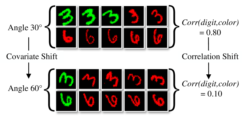
Many types of distribution shift are introduced in (Lin et al., 2024), such as label shift (Wang et al., 2003), concept shift (Widmer and Kubat, 1996), covariate shift (Shimodaira, 2000), and correlation shift (Roh et al., 2023). The covariate shift is defined as the differences in the marginal distributions over instances across different domains (Shimodaira, 2000). As shown in Figure 1, the two domains exhibit variations resulting from different image styles, represented by varying rotation angles. Correlation shift is defined as the variation in the dependency between the sensitive attribute and label across domains. For example, in Figure 1, it is evident that there is a strong correlation between the digit (3,6) and digit colors (green, red) when rotated at , whereas this correlation becomes less pronounced at .
Since the correlation involves sensitive attributes, correlation shift is highly related to fairness. In the context of algorithmic decision-making, fairness means the absence of any bias or favoritism towards an individual or group based on their inherent or acquired characteristics (Mehrabi et al., 2021). Many methods have been proposed to address the domain generalization (DG) problem (Arjovsky et al., 2019; Li et al., 2018b, 2023; Sun and Saenko, 2016; Zhang et al., 2022), but most of them lack fairness considerations. Therefore, when these algorithms are applied in human-centered real-world settings, they may exhibit bias against populations (Kang and Tong, 2021) characterized by sensitive features, such as gender and race.
While existing efforts have addressed the challenge of fairness-aware domain generalization due to shifted domains, they either overlook the variation in data across domains in the marginal distribution of data features (Creager et al., 2021; Oh et al., 2022) or specifically address the spurious correlation between sensitive attributes and predicted outcomes in terms of unchanged group fairness (Pham et al., 2023) across domains. Therefore, research is needed to explore fairness-aware domain generalization considering both covariate and correlation shifts simultaneously across training and test domains.
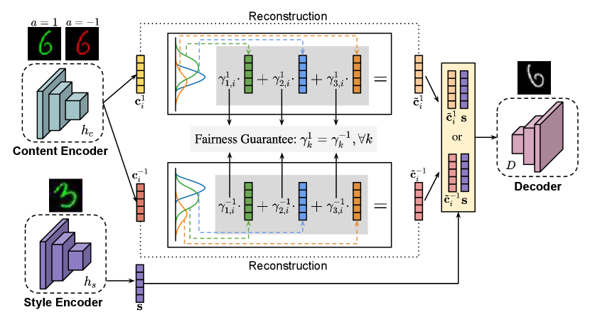
In this paper, we propose a novel framework, namely Fairness-aware LeArning Invariant Representations (FLAIR). It focuses on the problem arising from both covariate shift and correlation shift while considering fairness. The overall framework is shown in Figure 2. In the presence of multiple training domains, our objective is to acquire a predictor that is both domain-invariant and fairness-aware. This enables effective generalization in unseen test domains while preserving both accuracy and fairness. We assume there exists an underlying transformation model that can transform instances sampled from one domain to another while keeping the class labels unchanged. Under this assumption, the predictor consists of three components: a content featurizer, a fair representation learner, and an invariant classifier. To achieve fairness, data are divided into different sensitive subgroups. Within each subgroup, content factors encoded from the content featurizer are reconstructed using latent prototypes. These reconstructed content representations over various sensitive subgroups are crafted with dual objectives: (1) minimizing the inclusion of sensitive information and (2) maximizing the preservation of non-sensitive information. Utilizing these representations as inputs, we train a fairness-aware domain-invariant classifier for making model predictions. Exhausted experiments showcase that FLAIR demonstrates robustness in the face of covariate shift, even when facing alterations in unfairness and correlation shift across domains. The main contributions are summarized:
-
•
We introduce a fairness-aware domain generalization problem within a framework that addresses both covariate and correlation shifts simultaneously, which has practical significance.
-
•
We introduce an end-to-end training approach aimed at learning a fairness-aware domain invariant predictor. We claim that the trained predictor can generalize effectively to unseen test domains that are unknown and inaccessible during training.
-
•
Comprehensive experiments on three benchmark datasets show that our proposed algorithm FLAIR significantly outperforms state-of-the-art baselines with respect to model accuracy as well as both group and individual fairness.
2. Related Work
Algorithmic Fairness in Machine Learning. In recent years, fairness in machine learning has gained widespread attention. In this field, there is a widely recognized trade-off: enhancing fairness may come at the cost of accuracy to some extent (Chen et al., 2018; Menon and Williamson, 2018). How to handle such a trade-off, especially in real-world datasets, has been a widely researched issue in the field of algorithmic fairness.
From a statistical perspective, algorithmic fairness metrics are typically divided into group fairness and individual fairness. The conflict between them is a common challenge, as algorithms that achieve group fairness may not be able to handle individual fairness (Lahoti et al., 2019). LFR (Zemel et al., 2013) is the first method to achieve both group fairness and individual fairness simultaneously. It encodes tabular data, aiming to preserve the original data as much as possible while ignoring information related to sensitive attributes.
Fairness-Aware Domain Generalization. Some efforts (Zhao et al., 2023, 2022; Zhao, 2021; Zhao et al., 2024, 2021) have already been attempted to address the fairness-aware domain generalization problem. EIIL (Creager et al., 2021) takes correlation shift into consideration when addressing the DG problem, thus ensuring fairness to some extent. FVAE (Oh et al., 2022) learns fair representation through contrastive learning and both improve out-of-distribution generalization and fairness. But both of them only take correlation shift into account while assuming that covariate shift remains invariant. The latest work FATDM (Pham et al., 2023) attempts to simultaneously enhance the model’s accuracy and fairness, considering the DG problem associated with covariate shift. However, it does not consider correlation shift and solely focuses on group fairness, without addressing individual fairness.
3. Preliminaries
Notations. Let denote a feature space, is a sensitive space, and is a label space for classification. Let and be the latent content and style spaces, respectively, induced from by an underlying transformation model . We use to denote random variables that take values in and be the realizations. A domain is specified by distribution . A predictor parameterized by denotes .
Problem Formulation. We consider a set of data domains , where each domain corresponds to a distinct data sampled i.i.d. from . Given a dataset , it is partitioned into a training dataset with multiple training domains and a test dataset with unknown test domains which are inaccessible during training. Therefore, given samples from finite training domains, we aim to learn a fairness-aware predictor at training that is generalizable on unseen test domains.
Problem 1 (Domain generalization concerning fairness).
Let be a finite subset of training domains and assume that for each , we have access to its corresponding data sampled i.i.d. from . Given a loss function , the goal is to learn a fair predictor parameterized by for any that minimizes the worst-case risk over training domains that
However, addressing Problem 1 by training such a predictor is challenging because (1) is required to remain invariant across domains in terms of model accuracy, and model outcomes are fair with respect to sensitive subgroups defined by ; and (2) we do not assume data from is accessible during training.
To tackle such challenges, we divide the fairness-aware domain invariant predictor into three components: a domain-invariant featurizer parameterized by , a fair representation learner parameterized by , and a classifier parameterized by , denoted and .
4. Fairness-aware Learning Invariant Representations (FLAIR)
In this paper, we narrow the scope of various distribution shifts and focus on a hybrid shift where covariate and correlation shifts are present simultaneously.
Definition 0 (Covariate shift and correlation shift).
Given and , a covariate shift occurs in Problem 1 when domain variation is due to differences in the marginal distributions over input features . Meanwhile, a correlation shift arises in Problem 1 when domain variation results from changes in the joint distribution between and , denoted as . More specifically, and ; or and .
In Section 4.1, we handle covariate shift by enforcing invariance on instances based on disentanglement, while in Section 4.2, we address correlation shift by learning fair content representation.
4.1. Disentanglement of Domain Variation
In (Robey et al., 2021), distribution shifts are attributed into two forms: concept shift, where the distribution of instance classes varies across different domains, and covariate shift, where the marginal distributions over instance are various. In this paper, we restrict the scope of our framework to focus on Problem 1 in which inter-domain variation is solely due to covariate shift.
Building upon the insights from existing domain generalization literature (Zhang et al., 2022; Robey et al., 2021; Zhao et al., 2023), data variations across domains are disentangled into multiple factors in latent spaces.
Assumption 1 (Latent Factors).
Given sampled i.i.d. from in domain , we assume that each instance is generated from
-
•
a latent content factor , where refers to a content space, and is a content encoder;
-
•
a latent style factor , where is specific to the individual domain , and is a style encoder.
We assume that the content factors in do not change across domains. Each domain over is represented by a unique and , where is the correlation betweem and .
Under Assumption 1, we further assume that, for any two domains , inter-domain variations between them due to covariate shift are managed via an underlying transformation model . Through this model, instances sampled from such two domains can be transformed interchangeably.
Assumption 2 (Transformation Model).
We assume, , there exists a function that transforms instances from domain to , denoted as . The transformation model is defined as
where and are content and style encoders defined in Assumption 1, and denotes a decoder.
With the transformation model that transforms instances from domain to , , under Assumption 2, we introduce a new definition of invariance with respect to the variation captured by in Definition 2.
Definition 0 (-invariance).
Definition 2 is crafted to enforce invariance on instances based on disentanglement via . The output of is further utilized to acquire a fairness-aware representation, considering different sensitive subgroups, through the learner within the content latent space.
4.2. Learning Fair Content Representations
Dwork et al., (Dwork et al., 2012) defines fairness that similar individuals are treated similarly. As stated in Section 4.1, the featurizer maps instances to the latent content space. Therefore, for each instance sampled i.i.d. from where , the goal of the learner is to reconstruct a fair content representation from , wherein is generated to meet two objectives (1) minimizing the information disclosure related to a specific sensitive subgroup or , and (2) maximizing the preservation of significant information within non-sensitive representations. Under Assumption 1, since the content space is invariant across domains, we omit the superscript of domain labels for content factors.
To achieve these objectives effectively through and drawing inspiration from (Zemel et al., 2013; Lahoti et al., 2019), we group the content factors along with the sensitive attributes, denoted , of instances within each sensitive subgroup , which are encoded from , into clusters based on their similarity. Consequently, their fair content representations , with the sensitive attributes unchanged, are reconstructed using weighted prototypes, with each prototype representing a statistical mean estimated from each cluster.
Specifically, for content factors in a sensitive subgroup where , let be a latent variable, where its realization is a -dimensional vector, satisfying a particular entry is equal to , while all other entries are set to s, and . We denote as the mixing coefficients representing the prior probability of that belongs to the -th prototype.
In the context of Gaussian mixture models, we assume the conditional distribution . To estimate the parameters of the subgroup , we take the loss
| (2) |
Intuitively, the latent variable is the key to finding the maximal log-likelihood. We attempt to compute the posterior distribution of given the observations :
| (3) |
To achieve fairness, the fundamental idea designing is to make sure that the probability that a random content factor from the sensitive subgroup mapping to the -th particular prototype is equal to the probability of a random content factor mapping to the prototype from the other sensitive subgroup .
| (4) |
We hence formulate the loss regarding fairness that
| (5) |
where . Eq.(5) draws inspiration from the group fairness metric, known as the Difference of Demographic Parity (DDP) (Lohaus et al., 2020), which enforces the statistical parity between two sensitive subgroups.
To maximize the non-sensitive information in the reconstructed content representations, the reconstruction loss is defined
| (6) | ||||
where and is the Euclidean distance metric.
4.3. Learning the Predictor
To tackle Problem 1, which aims to learn a fairness-aware domain invariant predictor , a crucial element of is the acquisition of content factors through , while simultaneously reducing the sensitive information associated with them through . In this subsection, we introduce a framework designed to train with a focus on both domain invariance and model fairness.
Given training domains , a data batch containing multiple quartet instance pairs are sampled from
and , , where denotes the number of quartet pairs in . Specifically,
We set and (same to and ) share the same domain but different class label and , while and (same to and ) share the same class label but different domains and . Therefore, and are alternative instances with respect to and in a different domain, respectively.
Note that in each distance metric of , it compares a pair of instances with the same domain but different classes.
Furthermore, given Eq.(2), Eq.(6) and under Definition 2, we have the invariant classification loss with respect to ,
| (8) |
with
where indicates a distance metric, such as -norm. indicates the empirical risk of instance pairs with the sensitive attribute . Similarly, is the empirical risk of instance pairs with the sensitive attribute . Notice that the instance pair in sampled from have the same class label but different domains, such as and .
Finally, the fair loss is defined over the data batch with all sensitive attributes using Eq.(5),
| (9) |
Therefore the total loss is given
| (10) |
where are Lagrangian multipliers.
4.4. An Effective Algorithm
| Define by encoding using and with respect to the sensitive subgroup |
We introduce an effective algorithm for FLAIR to implement the predictor , as shown in Algorithm 1. Lines 2-3 represent the transformation model , while lines 4-6 denote the fair representation learner . In the component, we employ as an approximation to , since the EM algorithm(McLachlan and Krishnan, 2007) in FairGMMs continuously estimates using , . Parameters of update are given in lines 15-18 of Algorithm 1. We optimize and in the using the primal-dual algorithm, which is an effective tool for enforcing invariance (Robey et al., 2021). The time complexity of Algorithm 1 is , where is the number of batches.
5. Experimental Settings
| Consisitency / / AUCfair / Accuracy | |||
| ERM (Vapnik, 1999) | 0.94 (0.03) / 0.04 (0.01) / 0.54 (0.01) / 92.02 (0.35) | 0.95 (0.05) / 0.32 (0.04) / 0.67 (0.01) / 98.34 (0.17) | 0.95 (0.03) / 0.15 (0.01) / 0.56 (0.01) / 97.99 (0.34) |
| IRM (Arjovsky et al., 2019) | 0.96 (0.01) / 0.04 (0.01) / 0.53 (0.01) / 90.67 (0.89) | 0.95 (0.05) / 0.32 (0.03) / 0.67 (0.01) / 97.94 (0.25) | 0.95 (0.02) / 0.15 (0.03) / 0.55 (0.01) / 97.65 (0.28) |
| GDRO (Sagawa et al., 2019) | 0.95 (0.01) / 0.04 (0.02) / 0.55 (0.01) / 93.00 (0.67) | 0.95 (0.02) / 0.31 (0.05) / 0.66 (0.01) / 98.07 (0.33) | 0.95 (0.04) / 0.16 (0.01) / 0.58 (0.01) / 97.84 (0.30) |
| Mixup (Yan et al., 2020) | 0.95 (0.01) / 0.04 (0.01) / 0.54 (0.01) / 93.27 (0.84) | 0.95 (0.05) / 0.31 (0.05) / 0.66 (0.01) / 98.13 (0.20) | 0.95 (0.05) / 0.16 (0.02) / 0.57 (0.01) / 98.26 (0.11) |
| MLDG (Li et al., 2018b) | 0.95 (0.01) / 0.04 (0.01) / 0.53 (0.01) / 92.37 (0.47) | 0.95 (0.03) / 0.31 (0.03) / 0.65 (0.01) / 97.65 (0.18) | 0.95 (0.05) / 0.16 (0.04) / 0.56 (0.01) / 98.07 (0.26) |
| CORAL (Sun and Saenko, 2016) | 0.95 (0.01) / 0.04 (0.01) / 0.55 (0.01) / 93.81 (0.82) | 0.96 (0.02) / 0.31 (0.03) / 0.67 (0.01) / 98.31 (0.44) | 0.96 (0.03) / 0.16 (0.05) / 0.58 (0.01) / 98.49 (0.29) |
| DANN (Ganin et al., 2016) | 0.94 (0.02) / 0.04 (0.01) / 0.54 (0.01) / 91.24 (2.11) | 0.93 (0.05) / 0.30 (0.02) / 0.63 (0.04) / 96.74 (0.27) | 0.93 (0.02) / 0.14 (0.01) / 0.54 (0.03) / 96.84 (0.34) |
| CDANN (Li et al., 2018a) | 0.94 (0.01) / 0.04 (0.01) / 0.53 (0.01) / 91.08 (1.21) | 0.93 (0.05) / 0.31 (0.02) / 0.66 (0.01) / 97.47 (0.32) | 0.93 (0.01) / 0.15 (0.01) / 0.57 (0.02) / 96.57 (0.66) |
| DDG (Zhang et al., 2022) | 0.97 (0.01) / 0.01 (0.01) / 0.50 (0.05) / 96.90 (0.11) | 0.96 (0.03) / 0.31 (0.04) / 0.65 (0.01) / 97.79 (0.05) | 0.97 (0.02) / 0.16 (0.01) / 0.59 (0.03) / 97.42 (0.33) |
| DIR (Feldman et al., 2015) | 0.73 (0.03) / 0.02 (0.05) / 0.52 (0.05) / 71.89 (0.21) | 0.73 (0.03) / 0.18 (0.03) / 0.57 (0.05) / 72.61 (0.24) | 0.72 (0.02) / 0.17 (0.04) / 0.56 (0.01) / 71.72 (0.11) |
| EIIL (Creager et al., 2021) | 0.93 (0.01) / 0.14 (0.04) / 0.58 (0.01) / 82.00 (0.76) | 0.96 (0.02) / 0.27 (0.03) / 0.63 (0.06) / 92.07 (0.18) | 0.96 (0.04) / 0.14 (0.01) / 0.61 (0.01) / 92.17 (0.28) |
| FVAE (Oh et al., 2022) | 0.95 (0.02) / 0.07 (0.03) / 0.53 (0.03) / 91.44 (2.02) | 0.96 (0.01) / 0.30 (0.02) / 0.59 (0.06) / 92.49 (1.42) | 0.96 (0.06) / 0.18 (0.05) / 0.60 (0.04) / 91.69 (6.34) |
| FATDM (Pham et al., 2023) | 0.94 (0.01) / 0.01 (0.01) / 0.52 (0.02) / 94.02 (1.02) | 0.95 (0.01) / 0.19 (0.01) / 0.55 (0.02) / 90.65 (1.42) | 0.94 (0.01) / 0.14 (0.02) / 0.55 (0.02) / 90.25 (1.36) |
| FLAIR | 0.97 (0.02) / 0.02 (0.01) / 0.52 (0.01) / 93.11 (1.23) | 0.99 (0.02) / 0.18 (0.02) / 0.56 (0.04) / 90.85 (1.56) | 0.99 (0.02) / 0.12 (0.03) / 0.54 (0.02) / 91.77 (1.94) |
| Avg | ||||
| ERM (Vapnik, 1999) | 0.95 (0.04) / 0.35 (0.05) / 0.69 (0.01) / 98.34 (0.12) | 0.95 (0.01) / 0.29 (0.02) / 0.68 (0.01) / 98.04 (0.18) | 0.93 (0.01) / 0.17 (0.02) / 0.62 (0.02) / 94.60 (0.46) | 0.946 / 0.221 / 0.626 / 96.55 |
| IRM (Arjovsky et al., 2019) | 0.96 (0.05) / 0.35 (0.01) / 0.69 (0.01) / 97.68 (0.42) | 0.96 (0.01) / 0.28 (0.01) / 0.66 (0.01) / 97.11 (0.47) | 0.93 (0.02) / 0.16 (0.02) / 0.61 (0.01) / 93.67 (0.30) | 0.953 / 0.217 / 0.619 / 95.79 |
| GDRO (Sagawa et al., 2019) | 0.95 (0.05) / 0.35 (0.01) / 0.71 (0.02) / 98.07 (0.30) | 0.96 (0.01) / 0.29 (0.01) / 0.69 (0.01) / 97.88 (0.39) | 0.93 (0.04) / 0.16 (0.01) / 0.61 (0.01) / 94.40 (0.41) | 0.952 / 0.220 / 0.631 / 96.54 |
| Mixup (Yan et al., 2020) | 0.95 (0.04) / 0.34 (0.03) / 0.69 (0.01) / 98.39 (0.22) | 0.96 (0.03) / 0.29 (0.04) / 0.68 (0.01) / 97.94 (0.14) | 0.93 (0.01) / 0.15 (0.01) / 0.59 (0.01) / 93.58 (0.61) | 0.951 / 0.215 / 0.623 / 96.59 |
| MLDG (Li et al., 2018b) | 0.95 (0.05) / 0.35 (0.01) / 0.70 (0.01) / 98.15 (0.07) | 0.96 (0.03) / 0.28 (0.04) / 0.66 (0.01) / 97.59 (0.15) | 0.94 (0.02) / 0.17 (0.04) / 0.62 (0.01) / 94.30 (0.36) | 0.952 / 0.219 / 0.620 / 96.36 |
| CORAL (Sun and Saenko, 2016) | 0.96 (0.05) / 0.35 (0.04) / 0.68 (0.01) / 98.63 (0.23) | 0.96 (0.05) / 0.29 (0.03) / 0.68 (0.01) / 98.33 (0.16) | 0.94 (0.01) / 0.16 (0.01) / 0.61 (0.02) / 95.43 (0.74) | 0.954 / 0.221 / 0.628 / 97.17 |
| DANN (Ganin et al., 2016) | 0.93 (0.02) / 0.35 (0.01) / 0.70 (0.01) / 97.36 (0.26) | 0.94 (0.04) / 0.29 (0.01) / 0.69 (0.01) / 97.03 (0.25) | 0.90 (0.01) / 0.17 (0.01) / 0.62 (0.01) / 90.60 (1.13) | 0.928 / 0.216 / 0.620 / 94.97 |
| CDANN (Li et al., 2018a) | 0.93 (0.03) / 0.35 (0.01) / 0.69 (0.02) / 97.61 (0.40) | 0.94 (0.02) / 0.29 (0.03) / 0.67 (0.01) / 97.60 (0.17) | 0.90 (0.02) / 0.18 (0.02) / 0.62 (0.01) / 90.63 (1.67) | 0.928 / 0.219 / 0.623 / 95.16 |
| DDG (Zhang et al., 2022) | 0.97 (0.02) / 0.35 (0.01) / 0.69 (0.05) / 97.97 (0.05) | 0.97 (0.03) / 0.28 (0.02) / 0.64 (0.05) / 97.81 (0.06) | 0.95 (0.03) / 0.15 (0.01) / 0.58 (0.01) / 96.74 (0.13) | 0.963 / 0.209 / 0.609 / 97.44 |
| DIR (Feldman et al., 2015) | 0.73 (0.04) / 0.22 (0.02) / 0.57 (0.03) / 72.35 (0.19) | 0.72 (0.04) / 0.21 (0.03) / 0.56 (0.03) / 70.85 (0.21) | 0.73 (0.02) / 0.16 (0.05) / 0.57 (0.01) / 69.69 (0.14) | 0.728 / 0.161 / 0.555 / 71.52 |
| EIIL (Creager et al., 2021) | 0.97 (0.03) / 0.26 (0.02) / 0.62 (0.01) / 91.83 (0.38) | 0.96 (0.02) / 0.27 (0.01) / 0.59 (0.01) / 93.09 (0.22) | 0.96 (0.02) / 0.21 (0.02) / 0.61 (0.01) / 93.77 (0.10) | 0.959 / 0.216 / 0.607 / 90.82 |
| FVAE (Oh et al., 2022) | 0.97 (0.01) / 0.28 (0.04) / 0.56 (0.02) / 92.85 (1.30) | 0.97 (0.01) / 0.28 (0.01) / 0.67 (0.03) / 91.02 (1.25) | 0.94 (0.02) / 0.21 (0.02) / 0.60 (0.03) / 91.34 (1.74) | 0.958 / 0.220 / 0.592 / 91.80 |
| FATDM (Pham et al., 2023) | 0.96 (0.04) / 0.25 (0.01) / 0.57 (0.02) / 92.90 (1.21) | 0.95 (0.02) / 0.26 (0.03) / 0.57 (0.01) / 91.72 (1.32) | 0.96 (0.01) / 0.14 (0.02) / 0.57 (0.03) / 91.11 (0.84) | 0.953 / 0.165 / 0.555 / 91.78 |
| FLAIR | 0.98 (0.02) / 0.28 (0.02) / 0.56 (0.03) / 92.05 (2.34) | 0.98 (0.02) / 0.24 (0.03) / 0.56 (0.04) / 91.95 (2.23) | 0.98 (0.01) / 0.11 (0.03) / 0.56 (0.04) / 91.55 (1.02) | 0.980 / 0.157 / 0.552 / 91.88 |
5.1. Datasets
Rotated-Colored-MNIST (RCMNIST) dataset is a synthetic image dataset generated from the MNIST dataset (LeCun et al., 1998) by rotating and coloring the digits. The rotation angles {,,,,,} of the digits are used to partition different domains, while the color of the digits is served as the sensitive attribute. A binary target label is created by grouping digits into and . To investigate the robustness of FLAIR in the face of correlation shift, we controlled the correlation between label and color for each domain in the generation process of RCMNIST, setting them respectively to . The correlation for domain was set to 0, implying that higher accuracy leads to fairer results.
New-York-Stop-and-Frisk (NYPD) dataset (Goel et al., 2016) is a real-world tabular dataset containing stop, question, and frisk data from some suspects in five different cities. We selected the full-year data from 2011, which had the highest number of stops compared to any other year. We consider the cities {BROOKLYN, QUEENS, MANHATTAN, BRONX, STATEN IS} where suspects were sampled as domains. The suspects’ gender serves as the sensitive attribute, and whether a suspect was frisked is treated as the target label.
FairFace dataset (Karkkainen and Joo, 2021) is a novel face image dataset containing 108,501 images labeled with race, gender, and age groups which is balanced on race. The dataset comprises face images from seven race group {White, Black, Latino/Hispanic, East Asian, Southeast Asian, Indian, Middle Eastern}. These race groups determine the domain to which an image belongs. Gender is considered a sensitive attribute, and the binary target label is determined based on whether the age is greater than 60 years old.
5.2. Evaluation Metrics
Given input feature , target label and binary sensitive attribute , we evaluate the algorithm’s performance on the test dataset . We measure the DG performance of the algorithm using Accuracy and evaluate the algorithm fairness using the following metrics.
Demographic parity difference () (Dwork et al., 2012) is a type of group fairness metric. Its rationale is that the acceptance rate provided by the algorithm should be the same across all sensitive subgroups. It can be formalized as
where is the predicted class label. The smaller the , the fairer the algorithm.
AUC for fairness () (Calders et al., 2013) is a pairwise group fairness metric. Define a scoring function , where represents the model parameters. The of measures the probability of correctly ranking positive examples ahead of negative examples.
where is an indicator function that returns 1 when the parameter is true and 0 otherwise. is divided into and based on , which respectively contain and samples. The value of ranges from 0 to 1, with a value closer to 0.5 indicating a fairer algorithm.
Consistency (Zemel et al., 2013) is an individual fairness metric based on the Lipschitz condition (Dwork et al., 2012). Specifically, Consistency measures the distance between each individual and its k-nearest neighbors.
where N is the total number of samples in , is the predicted class label for sample , and 111Note that in (Zemel et al., 2013), is applied to the full set of samples. To adapt it for DG task, here we apply it only to the set for the domain in which the samples are located. takes the features of sample as input and returns the set of indices corresponding to its k-nearest neighbors in the feature space. A larger Consistency indicates a higher level of individual fairness.
| Consisitency / / AUCfair / Accuracy | |||
| BROOKLYN | QUEENS | MANHATTAN | |
| ERM (Vapnik, 1999) | 0.92 (0.03) / 0.14 (0.01) / 0.60 (0.03) / 62.57 (0.15) | 0.92 (0.03) / 0.11 (0.01) / 0.58 (0.03) / 61.47 (0.15) | 0.91 (0.03) / 0.13 (0.04) / 0.60 (0.03) / 60.60 (0.16) |
| IRM (Arjovsky et al., 2019) | 0.93 (0.02) / 0.17 (0.01) / 0.62 (0.05) / 62.54 (0.07) | 0.92 (0.03) / 0.13 (0.01) / 0.60 (0.01) / 61.80 (0.38) | 0.92 (0.01) / 0.15 (0.01) / 0.61 (0.01) / 61.10 (0.13) |
| GDRO (Sagawa et al., 2019) | 0.93 (0.01) / 0.14 (0.01) / 0.60 (0.04) / 62.10 (0.17) | 0.92 (0.01) / 0.12 (0.01) / 0.59 (0.04) / 61.94 (0.30) | 0.92 (0.01) / 0.15 (0.01) / 0.60 (0.01) / 60.50 (0.07) |
| Mixup (Yan et al., 2020) | 0.92 (0.03) / 0.13 (0.01) / 0.59 (0.01) / 62.24 (0.30) | 0.92 (0.01) / 0.10 (0.01) / 0.58 (0.01) / 62.34 (0.98) | 0.92 (0.01) / 0.13 (0.01) / 0.60 (0.01) / 60.17 (0.38) |
| MLDG (Li et al., 2018b) | 0.93 (0.03) / 0.14 (0.01) / 0.60 (0.02) / 62.54 (0.13) | 0.92 (0.04) / 0.11 (0.01) / 0.58 (0.01) / 61.45 (0.23) | 0.92 (0.04) / 0.13 (0.05) / 0.60 (0.05) / 60.53 (0.18) |
| CORAL (Sun and Saenko, 2016) | 0.93 (0.02) / 0.15 (0.01) / 0.61 (0.01) / 62.38 (0.10) | 0.92 (0.01) / 0.11 (0.04) / 0.58 (0.01) / 61.51 (0.40) | 0.91 (0.02) / 0.13 (0.01) / 0.60 (0.01) / 60.61 (0.15) |
| DANN (Ganin et al., 2016) | 0.92 (0.01) / 0.15 (0.02) / 0.61 (0.01) / 61.78 (0.32) | 0.92 (0.02) / 0.11 (0.01) / 0.58 (0.01) / 61.06 (1.33) | 0.91 (0.05) / 0.15 (0.02) / 0.60 (0.01) / 60.51 (0.57) |
| CDANN (Li et al., 2018a) | 0.93 (0.05) / 0.15 (0.01) / 0.60 (0.01) / 62.07 (0.27) | 0.92 (0.02) / 0.11 (0.01) / 0.58 (0.01) / 61.28 (1.56) | 0.91 (0.04) / 0.15 (0.01) / 0.61 (0.01) / 60.59 (0.36) |
| DDG (Zhang et al., 2022) | 0.94 (0.02) / 0.14 (0.01) / 0.60 (0.02) / 62.46 (0.11) | 0.94 (0.02) / 0.11 (0.01) / 0.58 (0.04) / 62.45 (0.13) | 0.94 (0.03) / 0.13 (0.01) / 0.60 (0.04) / 61.11 (0.29) |
| DIR (Feldman et al., 2015) | 0.87 (0.03) / 0.14 (0.01) / 0.58 (0.05) / 57.23 (0.04) | 0.89 (0.01) / 0.10 (0.04) / 0.58 (0.05) / 55.80 (0.23) | 0.88 (0.02) / 0.11 (0.02) / 0.57 (0.02) / 56.19 (0.11) |
| EIIL (Creager et al., 2021) | 0.94 (0.03) / 0.11 (0.01) / 0.59 (0.01) / 59.92 (1.16) | 0.94 (0.02) / 0.10 (0.01) / 0.58 (0.01) / 56.06 (0.24) | 0.93 (0.05) / 0.04 (0.01) / 0.55 (0.01) / 53.08 (0.98) |
| FVAE (Oh et al., 2022) | 0.95 (0.01) / 0.12 (0.01) / 0.61 (0.01) / 58.78 (0.88) | 0.96 (0.02) / 0.13 (0.01) / 0.58 (0.01) / 58.76 (3.17) | 0.94 (0.01) / 0.13 (0.01) / 0.61 (0.03) / 60.63 (2.95) |
| FATDM (Pham et al., 2023) | 0.93 (0.01) / 0.09 (0.01) / 0.58 (0.02) / 60.13 (1.10) | 0.93 (0.02) / 0.05 (0.02) / 0.56 (0.01) / 58.48 (0.57) | 0.94 (0.01) / 0.12 (0.01) / 0.57 (0.01) / 57.02 (0.63) |
| FLAIR | 0.96 (0.01) / 0.10 (0.02) / 0.58 (0.01) / 58.08 (1.08) | 0.96 (0.04) / 0.03 (0.02) / 0.57 (0.01) / 60.82 (0.55) | 0.95 (0.02) / 0.10 (0.01) / 0.56 (0.02) / 58.14 (0.44) |
| BRONX | STATEN IS | Avg | |
| ERM (Vapnik, 1999) | 0.90 (0.01) / 0.03 (0.03) / 0.55 (0.04) / 61.07 (0.46) | 0.91 (0.03) / 0.15 (0.01) / 0.61 (0.01) / 67.02 (0.30) | 0.910 / 0.113 / 0.588 / 62.55 |
| IRM (Arjovsky et al., 2019) | 0.91 (0.04) / 0.06 (0.04) / 0.55 (0.02) / 59.84 (1.83) | 0.91 (0.01) / 0.17 (0.01) / 0.62 (0.01) / 66.68 (0.16) | 0.916 / 0.136 / 0.598 / 62.39 |
| GDRO (Sagawa et al., 2019) | 0.91 (0.04) / 0.04 (0.03) / 0.53 (0.02) / 60.94 (1.73) | 0.91 (0.04) / 0.15 (0.01) / 0.60 (0.01) / 66.48 (0.20) | 0.914 / 0.121 / 0.585 / 62.39 |
| Mixup (Yan et al., 2020) | 0.90 (0.02) / 0.07 (0.02) / 0.56 (0.01) / 61.30 (1.96) | 0.91 (0.02) / 0.14 (0.01) / 0.59 (0.05) / 66.25 (0.85) | 0.914 / 0.113 / 0.583 / 62.46 |
| MLDG (Li et al., 2018b) | 0.91 (0.05) / 0.03 (0.01) / 0.53 (0.02) / 60.94 (2.43) | 0.91 (0.04) / 0.15 (0.04) / 0.61 (0.03) / 66.94 (0.25) | 0.916 / 0.113 / 0.585 / 62.48 |
| CORAL (Sun and Saenko, 2016) | 0.91 (0.01) / 0.04 (0.03) / 0.54 (0.02) / 61.52 (3.13) | 0.91 (0.02) / 0.15 (0.01) / 0.60 (0.02) / 67.08 (0.21) | 0.917 / 0.114 / 0.586 / 62.62 |
| DANN (Ganin et al., 2016) | 0.88 (0.03) / 0.10 (0.01) / 0.56 (0.02) / 58.32 (1.28) | 0.91 (0.03) / 0.14 (0.01) / 0.60 (0.01) / 65.62 (0.18) | 0.910 / 0.130 / 0.591 / 61.46 |
| CDANN (Li et al., 2018a) | 0.90 (0.02) / 0.09 (0.03) / 0.56 (0.02) / 61.26 (1.25) | 0.91 (0.05) / 0.17 (0.01) / 0.61 (0.01) / 66.07 (0.59) | 0.914 / 0.132 / 0.594 / 62.25 |
| DDG (Zhang et al., 2022) | 0.93 (0.03) / 0.02 (0.02) / 0.53 (0.01) / 64.91 (0.57) | 0.93 (0.04) / 0.15 (0.01) / 0.60 (0.01) / 66.46 (0.22) | 0.935 / 0.109 / 0.582 / 63.48 |
| DIR (Feldman et al., 2015) | 0.90 (0.04) / 0.08 (0.02) / 0.58 (0.03) / 54.25 (0.17) | 0.89 (0.03) / 0.11 (0.02) / 0.56 (0.01) / 55.19 (0.11) | 0.883 / 0.107 / 0.577 / 55.73 |
| EIIL (Creager et al., 2021) | 0.92 (0.04) / 0.03 (0.02) / 0.53 (0.01) / 61.02 (1.14) | 0.94 (0.02) / 0.13 (0.01) / 0.55 (0.01) / 56.69 (0.98) | 0.933 / 0.080 / 0.561 / 57.35 |
| FVAE (Oh et al., 2022) | 0.93 (0.04) / 0.04 (0.01) / 0.54 (0.01) / 61.08 (1.16) | 0.93 (0.02) / 0.16 (0.01) / 0.56 (0.03) / 63.96 (1.58) | 0.941 / 0.115 / 0.578 / 60.64 |
| FATDM (Pham et al., 2023) | 0.94 (0.02) / 0.01 (0.02) / 0.54 (0.01) / 62.57 (0.59) | 0.93 (0.05) / 0.14 (0.01) / 0.57 (0.02) / 62.80 (1.83) | 0.931 / 0.082 / 0.566 / 60.20 |
| FLAIR | 0.94 (0.01) / 0.02 (0.02) / 0.52 (0.01) / 63.87 (1.14) | 0.95 (0.05) / 0.12 (0.01) / 0.55 (0.03) / 62.63 (1.06) | 0.955 / 0.073 / 0.560 / 60.71 |
5.3. Compared Methods
We validate the utility of FLAIR in handling Problem 1 using 13 methods. ERM (Vapnik, 1999), IRM (Arjovsky et al., 2019), GDRO (Sagawa et al., 2019), Mixup (Yan et al., 2020), MLDG (Li et al., 2018b), CORAL (Sun and Saenko, 2016), DANN (Ganin et al., 2016), CDANN (Li et al., 2018a), and DDG (Zhang et al., 2022) are DG methods without fairness consideration. Among them, DDG is a recently proposed method that focuses on learning invariant representations through disentanglement. DIR (Feldman et al., 2015) is a classic group fairness algorithm. EIIL (Creager et al., 2021) and FVAE (Oh et al., 2022) can achieve both domain generalization under correlation shift and fairness. FATDM (Pham et al., 2023) is the latest work that explicitly focuses on both domain generalization under covariate shift and group fairness simultaneously.
6. Results
To evaluate the performance of FLAIR, we posed the following research questions from shallow to deep and answered them in Sections 6.1, 6.3 and 6.2.
-
•
Q1) Can FLAIR effectively address Problem 1, or in other words, can FLAIR ensure both group fairness and individual fairness on unseen domains while maximizing DG performance?
-
•
Q2) Does FLAIR exhibit a good trade-off between DG performance and fairness?
-
•
Q3) What are the roles of the transformation model and the fair representation learner in FLAIR?
-
•
Q4) How is ensuring algorithmic fairness in the learning process of FLAIR?
6.1. Overall Performance
The overall performance of FLAIR and its competing methods on three real-world datasets is presented in Table 1, 2 and 3, means higher is better, means lower is better. Each experiment was conducted five times and the average results were recorded, with standard deviations reported in parentheses.
Fairness Evaluation. Focus on the average of each fairness metric across all domains, FLAIR almost achieves the best performance on all three datasets. Excluding DIR, which is not competitive due to its poor DG performance, FLAIR consistently ranks as either the fairest or the second fairest in each domain. This indicates its relative stability in achieving fairness across various domains compared to competing methods. All of the above analyses shows that FLAIR is able to achieve both individual fairness and group fairness on unseen domains with state-of-the-art results.
DG Evaluation Considering Trade-off. Considering the accur- acy-fairness trade-off, we aim to enhance DG performance while simultaneously ensuring algorithmic fairness. From this perspective, we notice that (i) methods solely focusing on DG cannot ensure algorithmic fairness effectively. (ii) Although lower than the above methods, the performance of DG for FLAIR is still competitive, and it outperforms other competing algorithms that also focus on fairness. (iii) On the FairFace dataset, FLAIR ensures the best fairness while its DG performance is second only to DDG. This is because the transformation model allows FLAIR to learn better domain-invariant representations when dealing with relatively complex data (facial photos) and types of environments.
Overall, FLAIR ensures fairness on both tabular and image data while maintaining strong DG capabilities. It can learn a fairness-aware domain-invariant predictor to effectively address Problem 1. The success of FLAIR on all three datasets, particularly RCMNIST, also demonstrates that our approach works effectively when dealing with DG problems involving covariate shift and correlation shift.
| Consisitency / / AUCfair / Accuracy | ||||
| White | Black | Latino/Hispanic | East Asian | |
| ERM (Vapnik, 1999) | 0.95 (0.02) / 0.05 (0.02) / 0.57 (0.01) / 92.97 (3.04) | 0.95 (0.01) / 0.03 (0.01) / 0.58 (0.01) / 91.31 (2.28) | 0.96 (0.04) / 0.02 (0.01) / 0.57 (0.02) / 95.33 (1.51) | 0.96 (0.03) / 0.02 (0.01) / 0.60 (0.01) / 96.71 (0.28) |
| IRM (Arjovsky et al., 2019) | 0.95 (0.01) / 0.05 (0.01) / 0.57 (0.01) / 93.26 (1.17) | 0.96 (0.01) / 0.02 (0.01) / 0.57 (0.01) / 92.94 (1.01) | 0.96 (0.03) / 0.03 (0.02) / 0.56 (0.03) / 94.85 (2.27) | 0.95 (0.01) / 0.03 (0.01) / 0.60 (0.01) / 95.23 (1.26) |
| GDRO (Sagawa et al., 2019) | 0.95 (0.01) / 0.06 (0.01) / 0.57 (0.01) / 91.94 (0.47) | 0.96 (0.01) / 0.02 (0.01) / 0.58 (0.01) / 92.67 (1.59) | 0.96 (0.01) / 0.01 (0.02) / 0.57 (0.01) / 96.14 (0.69) | 0.96 (0.01) / 0.02 (0.01) / 0.61 (0.01) / 96.63 (0.30) |
| Mixup (Yan et al., 2020) | 0.95 (0.04) / 0.05 (0.01) / 0.55 (0.05) / 92.29 (2.26) | 0.95 (0.01) / 0.03 (0.01) / 0.53 (0.01) / 92.49 (2.20) | 0.96 (0.03) / 0.02 (0.03) / 0.54 (0.03) / 95.42 (1.02) | 0.96 (0.01) / 0.03 (0.01) / 0.55 (0.02) / 96.09 (1.43) |
| MLDG (Li et al., 2018b) | 0.95 (0.05) / 0.05 (0.01) / 0.58 (0.01) / 93.71 (0.41) | 0.95 (0.04) / 0.02 (0.01) / 0.58 (0.01) / 93.21 (0.40) | 0.96 (0.03) / 0.02 (0.02) / 0.58 (0.01) / 95.64 (0.93) | 0.95 (0.03) / 0.02 (0.01) / 0.59 (0.02) / 96.34 (0.84) |
| CORAL (Sun and Saenko, 2016) | 0.95 (0.05) / 0.07 (0.02) / 0.57 (0.01) / 91.99 (2.14) | 0.95 (0.04) / 0.05 (0.01) / 0.57 (0.01) / 89.44 (2.35) | 0.95 (0.05) / 0.04 (0.01) / 0.56 (0.01) / 93.97 (0.57) | 0.95 (0.02) / 0.04 (0.01) / 0.57 (0.03) / 94.84 (0.99) |
| DANN (Ganin et al., 2016) | 0.93 (0.04) / 0.11 (0.01) / 0.59 (0.01) / 80.72 (2.23) | 0.92 (0.01) / 0.09 (0.01) / 0.58 (0.01) / 74.07 (1.65) | 0.93 (0.04) / 0.09 (0.02) / 0.61 (0.04) / 87.17 (2.48) | 0.92 (0.02) / 0.10 (0.02) / 0.60 (0.01) / 85.42 (3.67) |
| CDANN (Li et al., 2018a) | 0.91 (0.05) / 0.12 (0.02) / 0.59 (0.01) / 76.13 (2.65) | 0.91 (0.03) / 0.08 (0.01) / 0.58 (0.01) / 76.43 (2.09) | 0.92 (0.01) / 0.06 (0.01) / 0.60 (0.01) / 91.03 (1.42) | 0.92 (0.02) / 0.08 (0.02) / 0.60 (0.01) / 89.09 (2.69) |
| DDG (Zhang et al., 2022) | 0.95 (0.04) / 0.04 (0.04) / 0.56 (0.01) / 96.25 (0.64) | 0.96 (0.05) / 0.03 (0.01) / 0.55 (0.01) / 97.26 (0.60) | 0.97 (0.03) / 0.01 (0.01) / 0.55 (0.02) / 98.15 (0.52) | 0.96 (0.03) / 0.02 (0.01) / 0.59 (0.01) / 98.37 (0.63) |
| DIR (Feldman et al., 2015) | 0.74 (0.04) / 0.02 (0.03) / 0.52 (0.05) / 76.14 (0.11) | 0.75 (0.04) / 0.03 (0.01) / 0.52 (0.03) / 76.31 (0.17) | 0.75 (0.04) / 0.03 (0.03) / 0.52 (0.02) / 76.65 (0.19) | 0.75 (0.01) / 0.03 (0.01) / 0.52 (0.04) / 77.42 (0.21) |
| EIIL (Creager et al., 2021) | 0.96 (0.01) / 0.01 (0.00) / 0.55 (0.01) / 89.92 (0.12) | 0.96 (0.05) / 0.00 (0.00) / 0.59 (0.01) / 96.79 (0.11) | 0.97 (0.05) / 0.11 (0.03) / 0.55 (0.01) / 83.76 (0.57) | 0.97 (0.05) / 0.07 (0.01) / 0.60 (0.03) / 86.35 (1.87) |
| FVAE (Oh et al., 2022) | 0.94 (0.01) / 0.05 (0.04) / 0.54 (0.02) / 90.36 (1.05) | 0.91 (0.02) / 0.03 (0.01) / 0.57 (0.04) / 89.63 (2.22) | 0.97 (0.02) / 0.03 (0.01) / 0.55 (0.01) / 93.30 (0.97) | 0.98 (0.01) / 0.05 (0.01) / 0.57 (0.02) / 91.44 (1.58) |
| FATDM (Pham et al., 2023) | 0.95 (0.01) / 0.02 (0.02) / 0.53 (0.03) / 96.23 (1.11) | 0.96 (0.01) / 0.02 (0.02) / 0.54 (0.01) / 95.82 (0.13) | 0.95 (0.01) / 0.02 (0.04) / 0.55 (0.02) / 95.38 (0.29) | 0.95 (0.03) / 0.01 (0.01) / 0.55 (0.04) / 96.31 (0.35) |
| FLAIR | 0.98 (0.01) / 0.02 (0.01) / 0.57 (0.01) / 96.56 (0.76) | 0.98 (0.01) / 0.01 (0.00) / 0.53 (0.01) / 97.60 (0.13) | 0.98 (0.01) / 0.00 (0.00) / 0.54 (0.01) / 98.31 (0.30) | 0.97 (0.02) / 0.00 (0.00) / 0.55 (0.01) / 97.36 (0.28) |
| Southeast Asian | Indian | Middle Eastern | Avg | |
| ERM (Vapnik, 1999) | 0.96 (0.03) / 0.01 (0.01) / 0.56 (0.01) / 94.42 (0.29) | 0.94 (0.04) / 0.01 (0.03) / 0.53 (0.02) / 94.66 (0.32) | 0.95 (0.02) / 0.04 (0.01) / 0.57 (0.02) / 93.42 (1.85) | 0.952 / 0.026 / 0.568 / 94.12 |
| IRM (Arjovsky et al., 2019) | 0.96 (0.05) / 0.01 (0.01) / 0.56 (0.01) / 94.56 (0.41) | 0.93 (0.04) / 0.02 (0.02) / 0.54 (0.02) / 94.27 (0.29) | 0.94 (0.04) / 0.04 (0.01) / 0.56 (0.01) / 93.95 (1.37) | 0.950 / 0.029 / 0.566 / 94.15 |
| GDRO (Sagawa et al., 2019) | 0.96 (0.01) / 0.02 (0.01) / 0.57 (0.02) / 94.26 (0.47) | 0.94 (0.02) / 0.02 (0.01) / 0.53 (0.01) / 93.99 (0.79) | 0.95 (0.03) / 0.04 (0.01) / 0.57 (0.01) / 93.87 (0.47) | 0.954 / 0.027 / 0.570 / 94.21 |
| Mixup (Yan et al., 2020) | 0.96 (0.04) / 0.01 (0.02) / 0.51 (0.01) / 94.55 (0.28) | 0.94 (0.01) / 0.03 (0.01) / 0.53 (0.01) / 93.76 (0.46) | 0.95 (0.05) / 0.04 (0.01) / 0.55 (0.02) / 93.83 (0.44) | 0.953 / 0.029 / 0.538 / 94.06 |
| MLDG (Li et al., 2018b) | 0.96 (0.05) / 0.01 (0.02) / 0.56 (0.02) / 94.62 (0.16) | 0.93 (0.03) / 0.02 (0.02) / 0.56 (0.02) / 94.68 (0.37) | 0.95 (0.03) / 0.03 (0.01) / 0.58 (0.01) / 94.57 (0.20) | 0.952 / 0.023 / 0.577 / 94.68 |
| CORAL (Sun and Saenko, 2016) | 0.96 (0.05) / 0.02 (0.01) / 0.54 (0.02) / 93.96 (0.74) | 0.93 (0.05) / 0.03 (0.01) / 0.54 (0.02) / 93.78 (0.45) | 0.94 (0.02) / 0.05 (0.01) / 0.56 (0.02) / 92.56 (0.73) | 0.949 / 0.043 / 0.558 / 92.93 |
| DANN (Ganin et al., 2016) | 0.91 (0.05) / 0.04 (0.01) / 0.56 (0.01) / 86.96 (1.54) | 0.90 (0.04) / 0.07 (0.01) / 0.58 (0.02) / 88.35 (1.85) | 0.92 (0.02) / 0.09 (0.02) / 0.60 (0.02) / 84.68 (3.25) | 0.918 / 0.082 / 0.590 / 83.91 |
| CDANN (Li et al., 2018a) | 0.93 (0.05) / 0.04 (0.02) / 0.55 (0.01) / 84.56 (2.98) | 0.91 (0.02) / 0.06 (0.03) / 0.56 (0.03) / 88.91 (3.54) | 0.93 (0.02) / 0.05 (0.04) / 0.58 (0.01) / 86.14 (5.08) | 0.918 / 0.070 / 0.581 / 84.61 |
| DDG (Zhang et al., 2022) | 0.97 (0.03) / 0.01 (0.02) / 0.54 (0.01) / 97.98 (0.21) | 0.94 (0.04) / 0.01 (0.01) / 0.54 (0.02) / 97.29 (0.46) | 0.95 (0.01) / 0.04 (0.04) / 0.55 (0.02) / 97.13 (0.68) | 0.959 / 0.023 / 0.554 / 97.49 |
| DIR (Feldman et al., 2015) | 0.75 (0.03) / 0.03 (0.04) / 0.52 (0.02) / 75.46 (0.20) | 0.74 (0.05) / 0.03 (0.01) / 0.52 (0.03) / 74.55 (0.31) | 0.75 (0.01) / 0.03 (0.03) / 0.52 (0.05) / 68.14 (4.08) | 0.748 / 0.027 / 0.521 / 74.95 |
| EIIL (Creager et al., 2021) | 0.97 (0.01) / 0.03 (0.01) / 0.54 (0.03) / 85.90 (0.82) | 0.96 (0.02) / 0.04 (0.01) / 0.55 (0.01) / 88.96 (0.57) | 0.96 (0.02) / 0.04 (0.02) / 0.56 (0.01) / 89.65 (0.26) | 0.966 / 0.044 / 0.561 / 88.76 |
| FVAE (Oh et al., 2022) | 0.95 (0.01) / 0.03 (0.01) / 0.52 (0.01) / 90.23 (1.43) | 0.96 (0.04) / 0.04 (0.01) / 0.54 (0.01) / 88.48 (1.18) | 0.96 (0.01) / 0.06 (0.01) / 0.55 (0.02) / 86.80 (2.15) | 0.954 / 0.041 / 0.550 / 90.04 |
| FATDM (Pham et al., 2023) | 0.95 (0.01) / 0.01 (0.01) / 0.53 (0.02) / 94.21 (1.45) | 0.95 (0.01) / 0.01 (0.05) / 0.54 (0.03) / 94.52 (1.09) | 0.95 (0.05) / 0.02 (0.01) / 0.54 (0.01) / 94.01 (0.58) | 0.954 / 0.017 / 0.539 / 95.21 |
| FLAIR | 0.98 (0.01) / 0.00 (0.00) / 0.51 (0.01) / 96.75 (1.12) | 0.98 (0.01) / 0.00 (0.00) / 0.53 (0.01) / 96.87 (0.12) | 0.97 (0.02) / 0.02 (0.00) / 0.54 (0.01) / 96.28 (0.89) | 0.976 / 0.007 / 0.537 / 97.10 |

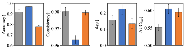
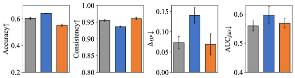
6.2. Ablation Study
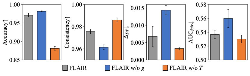
To understand the roles of the transformation model and the fair representation learner in learning a fairness-aware domain invariant predictor, we constructed two different variants of FLAIR for experimentation. They are: (i) FLAIR w/o g: remove , i.e., learn a predictor . (ii) FLAIR w/o T: replace with a standard featurizer and modify the corresponding input and output dimensions of and , i.e., learn a predictor The results of ablation study for FLAIR and its two variants on three dataset are shown in Figure 3 (a), (b) and (c).
By comparing FLAIR with its variant FLAIR w/o , we can see that the representations obtained by exhibit strong domain invariance but do not ensure fairness. Additionally, the improvement of FLAIR on all three fairness metrics suggests that can simultaneously enhance individual and group fairness. The difference between the results of them further validates the accuracy-fairness trade-off .
Contrasting FLAIR with its variant FLAIR w/o further highlights the DG utility of . At the same time, it’s evident that while focuses only on fairness, it doesn’t necessarily result in fairer outcomes. The reason for this is that the fair representation obtained solely through lacks domain invariance. As a result, it cannot handle covariate shift and correlation shift when generalizing to unseen domains.
The Utility of To understand how the critical component in promotes algorithmic fairness, we created two new variants of FLAIR. They are (i) FLAIR : removing from and (ii) FLAIR -: replacing the primal-dual updates with fixed parameters . Figure 4 shows the visualization of the fair content representations obtained by and its two variants on RCMNIST, organized by the respective sensitive subgroups.
The transition from (a) to (b) and (c) clearly shows that during optimization brings the representations of the two sensitive subgroups closer in the latent space, ensuring that similar individuals from different groups get more similar representations. Additionally, the clustering of each sensitive subgroup can bring closer the distances between similar individuals within the same group. Combining above two points, enables FLAIR to achieve a strong individual fairness effect. At the same time, enforces statistical parity between sensitive subgroups, reducing the distances between corresponding prototypes of different groups. This also ensures that FLAIR achieves group fairness. The transition from (b) to (c) shows that optimizing through the primal-dual algorithm is able to achieve better algorithmic fairness performance.
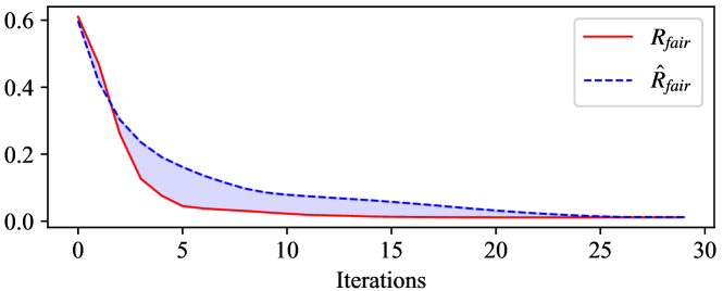
The convergence curves for both and during training are shown in Figure 5. Since the prior updates are not fully synchronized with the posterior updates (as seen in line 19 of Algorithm 1), a gap (indicated by the light blue area) exists between the two curves. However, their convergence trends are consistent, indicating that during training, can successfully approximate and does not affect the successful convergence of .
6.3. Sensitive Analysis
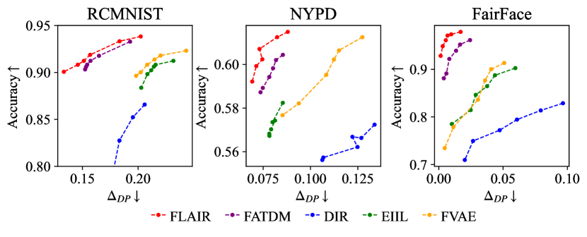
Accuracy-fairness Trade-off. To assess the trade-off performance of FLAIR, we obtained different group fairness and DG results of FLAIR by controlling the value of (larger implies FLAIR focuses more on algorithmic fairness). We compare the results with other fairness-aware methods, as shown in Figure 6 for all three datasets. It can be seen that the curve of the results obtained by FLAIR under different fairness levels is positioned in the upper-left corner among all methods. This indicates that FLAIR, while ensuring the best fairness performance, also maintains comparable domain generalization performance, achieving the best accuracy-fairness trade-off. Moreover, we observe that FLAIR achieves excellent fairness performance with comparable accuracy across all three datasets when . Therefore, we adopt this setting for all three datasets.
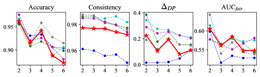
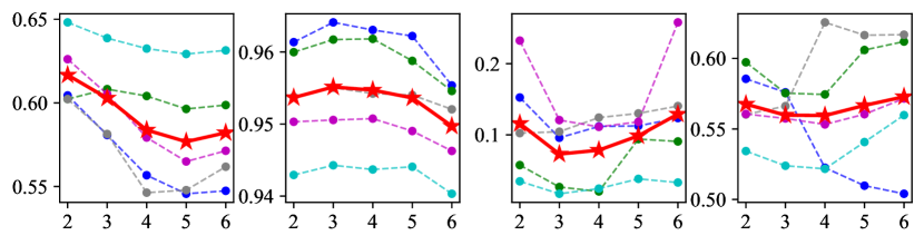
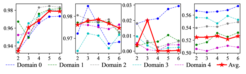
Number of Prototypes. To determine the number of prototypes in , we conducted a sensitivity analysis of . The experimental results on three datasets with fixed other parameters and varying values of from 2 to 6 are shown in Figure 7. The number of prototypes we ultimately selected on the three datasets is 3, 3 and 4. Because at these values, FLAIR had the highest average ranking across the four metrics as well as the best accuracy-fairness trade-off.
7. Conclusion
In this paper, we introduce a novel approach to fairness-aware learning that tackles the challenges of generalization from observed training domains to unseen testing domains. In our pursuit of learning a fairness-aware invariant predictor across domains, we assert the existence of an underlying transformation model that can transform instances from one domain to another. To ensure prediction with fairness between sensitive subgroups, we present a fair representation approach, wherein latent content factors encoded from the transformation model are reconstructed while minimizing sensitive information. We present a practical and tractable algorithm. Exhaustive empirical studies showcase the algorithm’s effectiveness through rigorous comparisons with state-of-the-art baselines.
Acknowledgements.
This work is supported by the NSFC program (No. 62272338).References
- (1)
- Arjovsky et al. (2019) Martin Arjovsky, Léon Bottou, Ishaan Gulrajani, and David Lopez-Paz. 2019. Invariant risk minimization. arXiv preprint arXiv:1907.02893 (2019).
- Calders et al. (2013) Toon Calders, Asim Karim, Faisal Kamiran, Wasif Ali, and Xiangliang Zhang. 2013. Controlling attribute effect in linear regression. In 2013 IEEE 13th international conference on data mining. IEEE, 71–80.
- Chen et al. (2018) Irene Chen, Fredrik D Johansson, and David Sontag. 2018. Why is my classifier discriminatory? Advances in neural information processing systems 31 (2018).
- Creager et al. (2021) Elliot Creager, Jörn-Henrik Jacobsen, and Richard Zemel. 2021. Environment inference for invariant learning. In International Conference on Machine Learning. PMLR, 2189–2200.
- Devlin et al. (2018) Jacob Devlin, Ming-Wei Chang, Kenton Lee, and Kristina Toutanova. 2018. Bert: Pre-training of deep bidirectional transformers for language understanding. arXiv preprint arXiv:1810.04805 (2018).
- Dwork et al. (2012) Cynthia Dwork, Moritz Hardt, Toniann Pitassi, Omer Reingold, and Richard Zemel. 2012. Fairness through awareness. In Proceedings of the 3rd innovations in theoretical computer science conference. 214–226.
- Feldman et al. (2015) Michael Feldman, Sorelle A Friedler, John Moeller, Carlos Scheidegger, and Suresh Venkatasubramanian. 2015. Certifying and removing disparate impact. In proceedings of the 21th ACM SIGKDD international conference on knowledge discovery and data mining. 259–268.
- Ganin et al. (2016) Yaroslav Ganin, Evgeniya Ustinova, Hana Ajakan, Pascal Germain, Hugo Larochelle, François Laviolette, Mario Marchand, and Victor Lempitsky. 2016. Domain-adversarial training of neural networks. The journal of machine learning research 17, 1 (2016), 2096–2030.
- Goel et al. (2016) Sharad Goel, Justin M Rao, and Ravi Shroff. 2016. Precinct or prejudice? Understanding racial disparities in New York City’s stop-and-frisk policy. (2016).
- Hu et al. (2022) Shishuai Hu, Zehui Liao, Jianpeng Zhang, and Yong Xia. 2022. Domain and content adaptive convolution based multi-source domain generalization for medical image segmentation. IEEE Transactions on Medical Imaging 42, 1 (2022), 233–244.
- Jin et al. (2020) Xin Jin, Cuiling Lan, Wenjun Zeng, and Zhibo Chen. 2020. Feature alignment and restoration for domain generalization and adaptation. arXiv preprint arXiv:2006.12009 (2020).
- Kang and Tong (2021) Jian Kang and Hanghang Tong. 2021. Fair graph mining. In Proceedings of the 30th ACM International Conference on Information & Knowledge Management. 4849–4852.
- Karkkainen and Joo (2021) Kimmo Karkkainen and Jungseock Joo. 2021. Fairface: Face attribute dataset for balanced race, gender, and age for bias measurement and mitigation. In Proceedings of the IEEE/CVF winter conference on applications of computer vision. 1548–1558.
- Krizhevsky et al. (2012) Alex Krizhevsky, Ilya Sutskever, and Geoffrey E Hinton. 2012. Imagenet classification with deep convolutional neural networks. Advances in neural information processing systems 25 (2012).
- Lahoti et al. (2019) Preethi Lahoti, Krishna P Gummadi, and Gerhard Weikum. 2019. ifair: Learning individually fair data representations for algorithmic decision making. In 2019 ieee 35th international conference on data engineering (icde). IEEE, 1334–1345.
- LeCun et al. (1998) Yann LeCun, Léon Bottou, Yoshua Bengio, and Patrick Haffner. 1998. Gradient-based learning applied to document recognition. Proc. IEEE 86, 11 (1998), 2278–2324.
- Li et al. (2023) Dong Li, Wenjun Wang, Minglai Shao, and Chen Zhao. 2023. Contrastive Representation Learning Based on Multiple Node-centered Subgraphs. In Proceedings of the 32nd ACM International Conference on Information and Knowledge Management. 1338–1347.
- Li et al. (2018b) Da Li, Yongxin Yang, Yi-Zhe Song, and Timothy Hospedales. 2018b. Learning to generalize: Meta-learning for domain generalization. In Proceedings of the AAAI conference on artificial intelligence, Vol. 32.
- Li et al. (2018a) Ya Li, Xinmei Tian, Mingming Gong, Yajing Liu, Tongliang Liu, Kun Zhang, and Dacheng Tao. 2018a. Deep domain generalization via conditional invariant adversarial networks. In Proceedings of the European conference on computer vision (ECCV). 624–639.
- Lin et al. (2024) Yujie Lin, Dong Li, Chen Zhao, Xintao Wu, Qin Tian, and Minglai Shao. 2024. Supervised Algorithmic Fairness in Distribution Shifts: A Survey. arXiv preprint arXiv:2402.01327 (2024).
- Lohaus et al. (2020) Michael Lohaus, Michael Perrot, and Ulrike Von Luxburg. 2020. Too relaxed to be fair. In International Conference on Machine Learning. PMLR, 6360–6369.
- McLachlan and Krishnan (2007) Geoffrey J McLachlan and Thriyambakam Krishnan. 2007. The EM algorithm and extensions. John Wiley & Sons.
- Mehrabi et al. (2021) Ninareh Mehrabi, Fred Morstatter, Nripsuta Saxena, Kristina Lerman, and Aram Galstyan. 2021. A survey on bias and fairness in machine learning. ACM computing surveys (CSUR) 54, 6 (2021), 1–35.
- Menon and Williamson (2018) Aditya Krishna Menon and Robert C Williamson. 2018. The cost of fairness in binary classification. In Conference on Fairness, accountability and transparency. PMLR, 107–118.
- Oh et al. (2022) Changdae Oh, Heeji Won, Junhyuk So, Taero Kim, Yewon Kim, Hosik Choi, and Kyungwoo Song. 2022. Learning fair representation via distributional contrastive disentanglement. In Proceedings of the 28th ACM SIGKDD Conference on Knowledge Discovery and Data Mining. 1295–1305.
- Pham et al. (2023) Thai-Hoang Pham, Xueru Zhang, and Ping Zhang. 2023. Fairness and accuracy under domain generalization. arXiv preprint arXiv:2301.13323 (2023).
- Robey et al. (2021) Alexander Robey, George J Pappas, and Hamed Hassani. 2021. Model-based domain generalization. Advances in Neural Information Processing Systems 34 (2021), 20210–20229.
- Roh et al. (2023) Yuji Roh, Kangwook Lee, Steven Euijong Whang, and Changho Suh. 2023. Improving fair training under correlation shifts. In International Conference on Machine Learning. PMLR, 29179–29209.
- Sagawa et al. (2019) Shiori Sagawa, Pang Wei Koh, Tatsunori B Hashimoto, and Percy Liang. 2019. Distributionally robust neural networks for group shifts: On the importance of regularization for worst-case generalization. arXiv preprint arXiv:1911.08731 (2019).
- Shimodaira (2000) Hidetoshi Shimodaira. 2000. Improving predictive inference under covariate shift by weighting the log-likelihood function. Journal of statistical planning and inference 90, 2 (2000), 227–244.
- Sun and Saenko (2016) Baochen Sun and Kate Saenko. 2016. Deep coral: Correlation alignment for deep domain adaptation. In Computer Vision–ECCV 2016 Workshops: Amsterdam, The Netherlands, October 8-10 and 15-16, 2016, Proceedings, Part III 14. Springer, 443–450.
- Vapnik (1999) Vladimir Vapnik. 1999. The nature of statistical learning theory. Springer science & business media.
- Wang et al. (2022) Jindong Wang, Cuiling Lan, Chang Liu, Yidong Ouyang, Tao Qin, Wang Lu, Yiqiang Chen, Wenjun Zeng, and Philip Yu. 2022. Generalizing to unseen domains: A survey on domain generalization. IEEE Transactions on Knowledge and Data Engineering (2022).
- Wang et al. (2003) Ke Wang, Senqiang Zhou, Chee Ada Fu, and Jeffrey Xu Yu. 2003. Mining changes of classification by correspondence tracing. In Proceedings of the 2003 SIAM International Conference on Data Mining. SIAM, 95–106.
- Wang et al. (2020) Wenhao Wang, Shengcai Liao, Fang Zhao, Cuicui Kang, and Ling Shao. 2020. Domainmix: Learning generalizable person re-identification without human annotations. arXiv preprint arXiv:2011.11953 (2020).
- Widmer and Kubat (1996) Gerhard Widmer and Miroslav Kubat. 1996. Learning in the presence of concept drift and hidden contexts. Machine learning 23 (1996), 69–101.
- Yan et al. (2020) Shen Yan, Huan Song, Nanxiang Li, Lincan Zou, and Liu Ren. 2020. Improve unsupervised domain adaptation with mixup training. arXiv preprint arXiv:2001.00677 (2020).
- Zemel et al. (2013) Rich Zemel, Yu Wu, Kevin Swersky, Toni Pitassi, and Cynthia Dwork. 2013. Learning fair representations. In International conference on machine learning. PMLR, 325–333.
- Zhang et al. (2022) Hanlin Zhang, Yi-Fan Zhang, Weiyang Liu, Adrian Weller, Bernhard Schölkopf, and Eric P Xing. 2022. Towards principled disentanglement for domain generalization. In Proceedings of the IEEE/CVF Conference on Computer Vision and Pattern Recognition. 8024–8034.
- Zhao (2021) Chen Zhao. 2021. Fairness-Aware Multi-Task and Meta Learning. Ph. D. Dissertation.
- Zhao et al. (2021) Chen Zhao, Feng Chen, and Bhavani Thuraisingham. 2021. Fairness-aware online meta-learning. In Proceedings of the 27th ACM SIGKDD Conference on Knowledge Discovery & Data Mining. 2294–2304.
- Zhao et al. (2022) Chen Zhao, Feng Mi, Xintao Wu, Kai Jiang, Latifur Khan, and Feng Chen. 2022. Adaptive fairness-aware online meta-learning for changing environments. In Proceedings of the 28th ACM SIGKDD Conference on Knowledge Discovery and Data Mining. 2565–2575.
- Zhao et al. (2024) Chen Zhao, Feng Mi, Xintao Wu, Kai Jiang, Latifur Khan, and Feng Chen. 2024. Dynamic Environment Responsive Online Meta-Learning with Fairness Awareness. ACM Transactions on Knowledge Discovery from Data 18, 6 (2024), 1–23.
- Zhao et al. (2023) Chen Zhao, Feng Mi, Xintao Wu, Kai Jiang, Latifur Khan, Christan Grant, and Feng Chen. 2023. Towards Fair Disentangled Online Learning for Changing Environments. In Proceedings of the 29th ACM SIGKDD Conference on Knowledge Discovery and Data Mining. 3480–3491.