Learning Expressive Priors for Generalization and
Uncertainty Estimation in Neural Networks
Abstract
In this work, we propose a novel prior learning method for advancing generalization and uncertainty estimation in deep neural networks. The key idea is to exploit scalable and structured posteriors of neural networks as informative priors with generalization guarantees. Our learned priors provide expressive probabilistic representations at large scale, like Bayesian counterparts of pre-trained models on ImageNet, and further produce non-vacuous generalization bounds. We also extend this idea to a continual learning framework, where the favorable properties of our priors are desirable. Major enablers are our technical contributions: (1) the sums-of-Kronecker-product computations, and (2) the derivations and optimizations of tractable objectives that lead to improved generalization bounds. Empirically, we exhaustively show the effectiveness of this method for uncertainty estimation and generalization.
1 Introduction
Within the deep learning approach to real-world AI problems such as autonomous driving, generalization and uncertainty estimation are one of the most important pillars. To achieve this, Bayesian Neural Networks (BNNs) (MacKay, 1992; Hinton & van Camp, 1993; Neal, 1996) leverage the tools of Bayesian statistics in order to improve generalization and uncertainty estimation in deep neural networks. Due to their potential and advancements so far, BNNs have become increasingly popular research topics (Gawlikowski et al., 2021). However, one of the open problems in BNNs is the prior specifications. While it is widely known that prior selection is a crucial step in any Bayesian modeling (Bayes, 1763), the choice of well-specified priors is generally unknown in neural networks. Consequently, many current approaches have resorted to uninformative priors, like isotropic Gaussian, despite reported signs of prior misspecifications (Wenzel et al., 2020; Fortuin, 2022).
To address the problem of prior specification, we propose a prior learning method for BNNs. Our method is grounded in sequential Bayesian inference (Opper, 1999), where the posteriors from the past are used as the prior for the future. We achieve this by relying on Laplace Approximation (LA) (MacKay, 1992) with Kronecker-factorization of the posteriors (Ritter et al., 2018b; Daxberger et al., 2021). Within this framework, we devise key technical novelties to learn expressive BNN priors with generalization guarantees. First, we demonstrate the sums-of-Kronecker-product computations so that the posteriors in matrix normal distributions, i.e., Gaussian with Kronecker-factorized covariance matrices (Gupta & Nagar, 2000), can be tractably used as expressive BNN priors. Second, to explicitly improve generalization, we derive and optimize over a tractable approximation of PAC-Bayes bounds (McAllester, 1999b; Germain et al., 2016) that lead to non-vacuous bounds, i.e., smaller than the upper bound of the loss. Finally, as an added benefit of our idea, a Bayesian re-interpretation to a popular continual learning architecture, namely progressive neural networks (Rusu et al., 2016), is provided for uncertainty-awareness, generalization, and resiliency to catastrophic forgetting.
By design, our method has many advantages for generalization and uncertainty estimation in neural networks. The proposed method achieves non-vacuous generalization bounds in deep learning models, while potentially avoiding prior misspecification for uncertainty estimation using BNNs. For these features, we provide computationally tractable techniques in order to learn expressive priors from large amounts of data and deep network architectures. We contend that such probabilistic representation at a large scale, e.g., pre-trained BNNs on ImageNet, can be beneficial in downstream tasks for both transfer and continual learning set-ups. Therefore, we further provide ablation studies and various experiments to show the aforementioned benefits of our method within the small and large-scale transfer and continual learning tasks. In particular, we empirically demonstrate that our priors mitigate cold posterior effects (Wenzel et al., 2020) – a potential sign of a bad prior – and further produce generalization bounds. Moreover, within a practical scenario of robotic continual learning (Denninger & Triebel, 2018), and standardized benchmarks of few-shot classification (Tran et al., 2022) for the recent uncertainty baselines (Nado et al., 2021), considerable performance improvements over the popular methods are reported.
Contributions To summarize, our primary contribution is a novel method for learning scalable and structured informative priors (Section 2), backed up by (a) the sums-of-Kronecker-product computations for computational tractability (Section 2.2), (b) derivation and optimizations over tractable generalization bounds (Section 2.3), (c) a Bayesian re-interpretation of progressive neural networks for continual learning (Section 2.4), (d) exhaustive experiments to show the effectiveness of our method (Section 4).
2 Learning Expressive Priors
2.1 Notation and Background
Consider a neural network with layers which consists of a parameterized function and a non-linear activation function . We denote an input for a network as and all learnable parameters as a stacked vector . Then the pre-activation and activation are recursively applied with , and . The output of the neural network is given by the last activation . The structure of the learning process is governed by different architectural choices such as fully connected, recurrent, and convolutional layers (Goodfellow et al., 2016). The parameters are typically obtained by maximum likelihood principles, given training data . Unfortunately, these principles lead to the lack of generalization and calibrated uncertainty in neural networks (Jospin et al., 2020).
To address these, BNNs provide a compelling alternative by applying Bayesian principles to neural networks. In BNNs, the first step is to specify a prior distribution . Then the Bayes theorem is used to compute the posterior distribution over the parameters, given the training data: . This means that each parameter is not a single value, but a probability distribution, representing the uncertainty of the model (Gawlikowski et al., 2021). The posterior distribution provides a set of plausible model parameters, which can be marginalized to compute the predictive distributions of a new sample for BNNs: . In the case of neural networks, the posteriors cannot be obtained in closed form. Hence, many of the current research efforts are on accurately approximating the posteriors of BNNs.
For this, LA (MacKay, 1992) approximates the BNN posteriors with a Gaussian distributions around a local mode. Here, a prior is first specified as an isotropic Gaussian. With this prior, the maximum-a-posteriori (MAP) estimates of the parameters are obtained by training the neural networks. Then, the Hessian is computed to obtain the BNN posteriors. In practice, the covariance matrix is usually further scaled which more generally corresponds to temperature scaling. In summary, the priors-posteriors pairs of LA are:
| (1) | ||||
As the Hessian is computationally intractable for modern architectures, the Kronecker-Factored Approximate Curvature (KFAC) method is widely adopted (Martens & Grosse, 2015). KFAC approximates the true Hessian by a layer-wise block-diagonal matrix, where each diagonal block is the Kronecker-factored Fisher matrix . Therefore, defining the layer-wise activation and loss gradient w.r.t pre-activation , the inverse covariance matrix of the posteriors is (Ritter et al., 2018b):
| (2) | ||||
In this way, using LA, BNN posteriors can be obtained by approximating the Hessian of neural networks. We provide more details on LA and KFAC in Section A.1.
We note several ramifications of this formulation for learning BNN priors from data. First, the BNN posteriors can be obtained by approximating the Hessian, which can be tractably computed from large amounts of data and deeper neural network architectures (Lee et al., 2020; Ba et al., 2017). Second, the resulting BNN posteriors can capture the correlations between the parameters within the same layer (Ritter et al., 2018b). Moreover, several open-source libraries exist to ease the implementations (Daxberger et al., 2021; Humt et al., 2020). All these points result in easily-obtainable BNN posteriors with expressive probabilistic representation from large amounts of data, deep architectures, and parameter correlations. As opposed to isotropic Gaussian, we next demonstrate that these BNN posteriors can be used to learn expressive prior distributions in order to advance generalization and uncertainty estimation within the transfer and continual learning set-ups.
2.2 Empirical Prior Learning with Sums-of-Kronecker-Product Computations
Intuitively, the idea is to repeat the LA with the prior chosen as the posterior from Equation 1, similar to Bayesian filtering. Since we use the LA with a Kronecker-factored covariance matrix in both the prior and the posterior, we want to approximate the resulting sum of Kronecker products with a single Kronecker product. We denote the task to compute the prior as source task and the task to compute the posterior as target task , both consisting of a data-set from a distribution , .
Applying LA on , we obtain the model parameters and the posteriors as before (equations 1 and 2). Then, for the target task, we specify the prior using the posteriors from : . The ultimate goal is to compute the new posteriors on , i.e., . To achieve this, we train the neural networks on by optimizing:
| (3) | |||||
where is the MAP estimate of the model parameters for task and is the block-diagonal Kronecker-factored Fisher matrix from task . The final step is to approximate new Hessian on using the KFAC method. This results in
| (4) | |||
where is the temperature scaling (Wenzel et al., 2020; Daxberger et al., 2021). Here, the precision matrix of the new BNN posteriors is represented by the sum-of-Kronecker-products, i.e., .
Unfortunately, the sum-of-Kronecker-products is not a Kronecker-factored matrix. As a result, the above formulation loses all the essence of Kronecker factorization for modeling high-dimensional probability distributions. For example, we can no longer exploit the rule: where and are smaller matrices to store and invert when compared to . Even more, the storage and the inverse of may not be computationally tractable for modern architectures.
To this end, we devise the sum-of-Kronecker-products computations. Concretely, we approximate the sum-of-Kronecker-products as Kronecker-factored matrices by an optimization formulation:111For the similar causes to maintain the Kronecker factorization, Ritter et al. (2018b, a) assume which does not hold in general (see Section 4.1).222Our formulation for one single Kronecker-factored matrix is similar to Kao et al. (2021).
| (5) |
A solution to this problem is not unique, e.g., one could scale by and by . Hence, we assume that is normalized, (or alternatively, we can also assume ). For the solution, we show the equivalence to the well-known best rank-one approximation problem.
Lemma 2.1.
Let , and for . Then
| (6) | ||||
Proof.
The proof can be found in Section C.1. ∎
This result indicates that the solution to equation 5 can be obtained using the power method, which iterates:
Given randomly initialized matrices, the power method iterates until the stop criterion is reached. The full procedure is presented in Algorithm 1, whereas in Appendix B, we discuss the computational complexity of the algorithm.
Importantly, we can now obtain a single Kronecker factorization from the sum of Kronecker products. Such Kronecker-factored approximations have advantages on tractable memory consumption for the storage and the inverse computations, which enables sampling from the resulting matrix normal distributions (Martens & Grosse, 2015). Therefore, such computations allow us to learn expressive BNN priors from the posterior distributions of previously encountered tasks. Finally, we can also prove the convergence of the power method to an optimal rank-one solution.
Lemma 2.2.
Let and be its singular value decomposition with and . Then there is a solution of Equation 5 with ,. If , the solution is unique up to changing the sign of both factors, and our power method converges almost surely to this solution.
Proof.
The proof can be found in Section C.2. ∎
2.3 Derivations and Optimizations over Tractable PAC-Bayes Bounds
So far, we have presented a method for learning a scalable and structured prior. In this section, we show how generalization bounds for the LA can be adapted to explicitly minimize the generalization bounds with the learned prior. In particular, the proposed approach allows tuning the hyperparameters of the LA on the training set without a costly grid search. This is achieved by optimizing a differentiable cost function that approximates generalization bounds for the LA. We choose to optimize generalization bounds to trade off the broadness of the distribution and the performance on the training data to improve generalization.
A common method in BNNs, and especially in LA, is to scale the covariance matrix by a positive scalar called the temperature (Wenzel et al., 2020; Daxberger et al., 2021). In addition, often either the Hessian (or Fisher matrix) of the likelihood (Ritter et al., 2018b; Lee et al., 2020) or the prior (Gawlikowski et al., 2021) is scaled. Including all these terms, the posterior has the following form:
| (7) |
where is the precision matrix of the prior. This reweighting of the three scalars allows us to cope with misspecified priors (Wilson & Izmailov, 2020), approximation errors in the Fisher matrices, and to improve the broadness of the distribution. While these values are usually hyperparameters that have to be manually scaled by hand, we argue that these values should be application-dependent. Therefore, we propose to find all three scales – , , and – by minimizing generalization bounds.
In the following, we will first introduce our two approaches and then explain how the optimization of PAC-Bayes bounds can be made tractable for the LA.
Method 1: Curvature Scaling Previous approaches typically scale only one or two of the scales (Daxberger et al., 2021; Ritter et al., 2018b; Lee et al., 2020). With our automatic scaling, we can optimize all three scales for each individual layer, allowing the model to decide the weighting in a more fine-grained way. We can use this method not only to scale the posterior, but also to compute the prior. Thus, the prior and posterior are defined as
| (8) |
where the diagonal blocks of the precision matrix corresponding to each layer are defined as and , respectively.
Remark 2.3.
Although the temperature scaling could be captured within the other curvature scales, we find it easier to optimize the bounds with all three parameters per layer.
Method 2: Frequentist Projection Going one step further, we propose to scale not only the curvature but also the network parameters using PAC-Bayes bounds. Since the Fisher matrix is known only after training, we assume the same covariance for the posterior as for the prior when optimizing the network parameters. Since this method does not optimize for the MAP parameters, but only for minimizing the PAC-Bayes bounds, we call it frequentist projection.
Both methods aim at improving the generalization of our model. To do this, we use PAC-Bayes bounds (Germain et al., 2016; Guedj, 2019) to derive a tractable objective that can be optimized without going through the data-set. The main idea of PAC-Bayes theory is to upper bound the expected loss on the true data distribution with high probability. The bounds typically depend on the expected empirical loss on the training data and the KL-divergence between a data-independent prior and the posterior distribution. For , that is
| (9) | ||||
where the loss on the true data distribution is denoted as and the empirical loss on the training data is . In general, the bounds balance the fit to the available data (empirical risk term) and the similarity of the posterior to the prior (the KL-divergence term), and the bounds hold with a probability greater than . Various forms of the bound can be found in the literature, with varying degrees of tightness. For classification, we rely on the McAllester (McAllester, 1999b) and Catoni (Catoni, 2007) bounds. 333This work focuses on classification tasks as PAC-Bayes framework is usually for bounded losses. Yet, using recent theories of PAC-Bayes, we also comment on regression in Appendix D.
Since these bounds depend on the expected empirical loss, we have to iterate over the entire training data and sample from the posterior multiple times at each step in order to evaluate the bound once. This makes optimization intractable. Using the error function as a loss, we propose to compute an approximate upper bound by only using quantities that were already computed during the LA, i.e. the Fisher matrix and the network parameters :
| (10) | ||||
where is from the precision matrix of the prior. Here, we first use a second-order Taylor approximation of around . Furthermore, the expectation can be converted to a trace by using the cyclic property of the trace together with the fact that the posterior is a multivariate Gaussian. The negative data log-likelihood of the optimal parameters can be computed jointly with the Fisher matrix during the LA. We denote this approximation as . On the other hand, the KL-divergence can also be computed in closed form for our prior-posterior pair, since both distributions are multivariate Gaussians. Thus, we can plug both terms into the McAllester bound (Guedj, 2019) to obtain the objective
| (11) |
where we write for the KL-divergence to emphasize the dependence on the scales. Similarly for the Catoni bound (Catoni, 2007), we obtain
| (12) |
Overall, these objectives can be evaluated and minimized without using any data samples. As opposed to the cross-validated marginal likelihood or other forms of grid searching, we (a) obtain generalization bounds and analysis, (b) do not need a separate validation set, (c) can find multiple hyperparameters, i.e., scale better with the dimensionality of the considered hyperparameters due to the differentiability of the proposed objectives, and (d) the complexity of the optimization is independent of the data set size and the complexity of the forward pass. The last point is because we only use the precomputed terms from the LA. A full derivation of our objective is given in Appendix C.
2.4 Bayesian Progressive Neural Networks
[width=]tikz/method/pbnn
| Method | Baseline | + grid Search | + learned prior | + curvature scaling | + frequentist projection |
|---|---|---|---|---|---|
| Catoni bound | |||||
| McAllester bound |
tikz/results/results_small_data_1e-5_1e-5
tikz/results/results_cold_posterior_1e-5
Having the essentials of learning BNN priors with generalization guarantees, we now present our extension to continual learning, which shows the versatility of our prior learning method. Here, we use so-called Progressive Neural Networks (PNNs) (Rusu et al., 2016), where a new neural network (column) is added for each new incoming task, and features from previous columns are also added for positive transfer between each task. Thus, PNNs are immune to catastrophic forgetting at the cost of an increase in memory, while being also applicable in transfer learning more generally (Wang et al., 2017; Rusu et al., 2017). As such, we extend the set-up in Section 2.2 by sequentially considering T tasks: . Moreover, to keep the generality of our method, an additional task is defined for the priors.
The idea behind our Bayesian re-interpretation of PNNs, dubbed as BPNNs for Bayesian PNNs, is as follows. First, the BNN posteriors are learned at task (depicted in Figure 1). Then, for an incoming sequence of tasks, the BNN priors are specified from the BNN posteriors from . The proposed methods of the sums-of-Kronecker-products and PAC-Bayes bounds are used. For the lateral connections, the BNN posterior from which the lateral connection originates is used. This ensures that the weight distribution from the prior already produces reasonable features given the activations from the previous column. Altogether, the resulting architecture accounts for model uncertainty, generalization, and resiliency to catastrophic forgetting. All these properties are desirable to have within one unified framework. We note that BPNN is in line with our PAC-Bayes theory, i.e., we increase the complexity without increasing the PAC-Bayes bounds. This is because we can reuse features from previous columns even though they do not contribute to the bounds due to their a-priori fixed weight distribution. In Appendices B and C, we provide more details such as its full derivations, and its training and testing procedures.
3 Related Work
There are different work streams related to this paper. The primary area is on BNN priors while we also contribute to Bayesian continual learning and PAC-Bayes theory.
| Iteration | 1 | 2 | 3 | 4 | 5 | 6 | 7 |
|---|---|---|---|---|---|---|---|
| Error |
[scale=0.95]tikz/appendix/results/skp_isotropic
Bayesian Neural Networks Priors A prior specification is a prerequisite in Bayesian modeling. However, for neural network parameters, the choice of the prior is generally unknown. So far, uninformative priors such as isotropic Gaussian have been the de-facto-standard for BNNs (Fortuin, 2022). Such uninformative priors may cause undesirable effects such as cold posteriors and worse predictive performance than standard neural networks (Wenzel et al., 2020; Fortuin et al., 2021). To this end, recent research efforts have focused on exploiting function-space (Sun et al., 2019), sparsity-inducing weight-space (Carvalho et al., 2009; Ghosh et al., 2018), structured (Louizos & Welling Max, 2016), and learning-based priors (Immer et al., 2021; Fortuin et al., 2021; Wu et al., 2019). Amongst these, we build upon learning-based priors. Learning-based priors can be an alternative to uninformative prior when no useful prior knowledge is available to encode, or when there exists relevant data and tasks to learn from (Fortuin, 2022).
The idea of learning a prior distribution on a similar task is certainly not new. In this domain, Bayesian meta-learning (Thrun & Pratt, 1998) and their modern extensions (Rothfuss et al., 2021a; Finn et al., 2018) can be viewed as another form of learning the prior from data, although their focus is typically not on advancing BNNs. Empirical prior learning is closely related to our work (Robbins, 1992). For BNNs, Fortuin et al. (2021) learns the empirical weight distributions during stochastic gradient descent. Wu et al. (2019) used a moment-matching approach, while Immer et al. (2021) exploited the so-called Laplace-Generalized-Gauss-Newton method. In (Krishnan et al., 2020), the mean of a Gaussian prior distribution is learned from a relevant data-set. The concurrent approaches of Shwartz-Ziv et al. (2022); Tran et al. (2022) share a similar spirit of learning expressive priors from large-scale data-set and architectures. The former utilizes so-called the SWAG (Maddox et al., 2019) framework with an inspiring idea of combining self-supervised learning, while the latter builds upon Frequentist batch ensembles (Wen et al., 2019). All these works show the strong relevance of learning-based priors for the current BNNs. Inspired by the aforementioned works, our main idea is to learn scalable and structured posterior as expressive informative priors, like Bayesian foundation models from broader data and models.
Bayesian Continual Learning Continual learning (Thrun & Mitchell, 1995) methods can be broadly divided into replay-based, regularization-based, and parameter-isolation methods (De Lange et al., 2022). We build on parameter-isolation methods, e.g. Rusu et al. (2016), where different model parameters are dedicated to new tasks. Within this branch, Bayesian methods have been investigated (Ebrahimi et al., 2020; Ardywibowo et al., 2022; Kumar et al., 2021), which could benefit from our work on advancing the BNN priors. Rudner et al. (2022) shares a similar spirit of bringing the state-of-the-art BNN priors to Bayesian continual learning by relying on the function space priors (Sun et al., 2019). On the other hand, using learning-based expressive priors, we design a single unified framework of continual learning for generalization, uncertainty-awareness, and resiliency to catastrophic forgetting.
Generalization Theory In supervised learning, we can obtain models with a bound on the true expected loss from its true data-generating process. Typical early works involved Vapnik-Chervonenkis theory and Rademacher complexity (Vapnik & Chervonenkis, 1968; Shalev-Shwartz & Ben-David, 2014). However, for high-dimensional models like neural networks, these methods often provide vacuous bounds. In recent years, PAC-Bayes theory (McAllester, 1999b; Germain et al., 2016) has become an alternative method with wide applications. The seminar paper of (Germain et al., 2016) showed the connection to approximate Bayesian inference. Rothfuss et al. (2021b, a) devise compelling meta-learning priors for BNNs with generalization guarantees. These works form our inspiration to explore PAC-Bayes theory for learning-based BNN priors. We note that our goal is not to advance PAC-Bayes theory, but to investigate a method for scaling the BNN priors with an approximate differentiable objective for generalization.
4 Results
The goal of the experiments is to investigate whether our approach provides generalization and calibrated uncertainty estimates. To this end, in addition to ablation studies on the presented algorithm, we show its utility for continual learning and uncertainty estimation. Implementation details are presented in Appendix E. The code is released at https://github.com/DLR-RM/BPNN.
| Other | Banana | Coffee Mug | Stapler | Flashlight | Apple | Average | |
|---|---|---|---|---|---|---|---|
| PNN (weight decay ) | |||||||
| PNN (weight decay ) | |||||||
| MC Dropout | |||||||
| zero mean & isotropic | |||||||
| isotropic | |||||||
| learned |
4.1 Ablation Studies
Our method is to improve generalization in the LA and also to provide an informative prior for the posterior inference. Therefore, in the ablation studies, we want to investigate the impact of each of our methods on the generalization bounds. Moreover, we want to study the learned prior in the small-data regime and see if it can mitigate the cold posterior effect, i.e. phenomena in BNNs where the performance improves by cooling the posterior with a temperature of less than one (Wenzel et al., 2020). This effect highlights the discrepancy of current BNNs, where no posterior tempering should be theoretically needed. For this, we use a LeNet-5 architecture (LeCun et al., 1989), learn the prior on MNIST (LeCun et al., 1998) and compute the posterior on NotMNIST (Bulatov, 2011). In our experiments, we compare the performance of our learned prior against an isotropic Gaussian prior with multiple weight decays, either with a mean zero or using the pre-trained model as the mean.
In Table 2(a), one can see the contribution of each method to the final generalization bounds. For this, we report the mean and standard deviation using different seeds. We observe that learning the prior improves the generalization bounds, as the posterior can reuse some of the pre-trained weights. The curvature further controls the flexibility of each parameter, leading to a smaller KL-divergence while still providing a small error rate. In addition, we show that scaling the curvature with our approximate bounds reduces the bounds. In particular, the generalization bounds are also better than a thorough grid search. Frequentist projection further leads to a non-vacuous bound of . In the small data regime, we train our method on a random subset of NotMNIST, i.e., we vary the number of available samples per class. Figure 2(b) shows that the learned prior requires a magnitude fewer data to achieve similar accuracy compared to isotropic priors. In Appendix F.2, we further evaluate the impact of using different temperature scalings and weight decays in this experiment. We observe larger improvements when the model is more probabilistic, i.e. when the temperature scaling is large, and when the weight decay is small and thus the learned prior is more dominant. Finally, following Wenzel et al. (2020), we examine the cold posterior effect using the learned prior in Figure 2(c). Although the optimal value for the temperature scaling is less than one, the temperature scaling can be closer to one compared to the isotropic priors. This suggests that the cold posterior effect is reduced by using a learned prior.
Additionally, we further validate the proposed sums-of-Kronecker product computations (see Figure 3). In Appendix F, further experimental results are provided, including qualitative analysis of our tractable approximate bound used to optimize the curvature scales (Appendix F.1). Furthermore, results for a larger cold posterior experiment using ResNet-50 (He et al., 2016), ImageNet-1K (Deng et al., 2009), and CIFAR-10 (Krizhevsky, 2009) are presented in Appendix F.3. Here, the learned prior improves the accuracy but does not reduce the cold posterior effect for all evaluated weight decays. This suggests the use-case of our method. Overall, our results demonstrate the effectiveness of our method in improving the generalization bounds. Furthermore, we show that the learned prior is particularly useful for BNNs when little data is available.
4.2 Generalization in Bayesian Continual Learning
Another advantage of our prior is its connection to continual learning. In the following experiments, we, therefore, evaluate our method for continual learning tasks. To do so, we closely follow the setup of Denninger & Triebel (2018), who introduces a practical robotics scenario. This allows us to also obtain meaningful results for practitioners. We do not use the typical MNIST setup here because we also want to test the effectiveness of the expressive prior from ImageNet (Deng et al., 2009). Each continual learning task consists of recognizing the specific object instances of the Washington RGB-D data-set (WRGBD) (Lai et al., 2011), while only a subset of all classes is available at a given time. We neglect the depth information and split the data similar to Denninger & Triebel (2018). The prior is learned with the ImageNet-1K (Deng et al., 2009) and the ResNet-50 (He et al., 2016) is used. We specify a total of four lateral connections, each at the downsampling convolution of the first ”bottleneck” building block of the ResNet layers. The baselines are PNNs with several weight decays and using MC dropout (Gal & Ghahramani, 2016). Moreover, we compare to both isotropic priors as in the ablations.
Table 1 shows the mean and the standard deviation of the accuracy for each task of the continual learning experiment for different random seeds. We report the mean and the standard deviation of two independent runs. Overall, in our experiments, the accuracy averaged over all tasks is improved by percent points compared to the second best approach PNN with weight decay . In addition, the increase in accuracy is percent points greater compared to an isotropic prior, and percent point greater when using zero as the prior mean. Therefore, these experimental results illustrate that with our idea of expressive posterior as BNN prior, we can improve the generalization on the test set for practical tasks of robotic continual learning.
4.3 Few-Shot Generalization and Uncertainty

Finally, we consider the task of few-shot learning. Our key hypothesis is that the choice of prior matters more in the small data regime, i.e., the prior may dominate over the likelihood term. To this end, closely following Tran et al. (2022), we use a few-shot learning set-up across several data-sets, namely CIFAR-100, UC Merced, Caltech 101, Oxford-IIIT Pets, DTD, Colorectal Histology, Caltech-UCSD Birds 200, and Cars196. CIFAR-10 is used as an out-of-distribution (OOD) data-set 444Unlike Tran et al. (2022), we did not use few-shot learning on ImageNet since we obtain our prior using the entire training set.. Standardized metrics such as accuracy, ECE, AUROC, and OOD AUROC are examined. The implementations are based on uncertainty baselines (Nado et al., 2021). We use ResNet-50 for the architecture.
For the baselines, we choose MC dropout (Gal & Ghahramani, 2016) (MCD) and additionally include deep ensemble (Lakshminarayanan et al., 2017) (Ens) and a standard network (NN). These uncertainty estimation techniques are often used methods in practice (Gustafsson et al., 2020). We do not use the plex (Tran et al., 2022) due to the lack of industry-level resources to comparably train our Bayesian prior. To increase their competitiveness, we uniformly searched over ten weight decays in the range from to . We also tried fixed representation or only last-layer fine-tuning. Additionally, we add LA which represents the use of isotropic prior. To facilitate the fair comparison between isotropic and learned prior, we carefully searched the following combinations: (a) curvature scaling without PAC-Bayes, with McAllester and Cantoni, (b) ten temperature scaling ranging from to , and (c) three weight decays to and . For all hyperparameters, we selected the best model using validation accuracy.
The results are reported in Figure 4, where we averaged across eight data-sets, closely following Tran et al. (2022). The results per data-set are in Appendix F.4 whereas in Appendix F.1, we also analyze the influence of these weight decays and temperature scales with varying numbers of available samples per class against accuracy. For shots up to 25 per class, we observe that our method often outperforms the baselines in terms of generalization and uncertainty calibration metrics. In particular, in the experiments, our learned prior from ImageNet significantly outperforms the isotropic prior within directly comparable set-ups. We interpret that the prior learning method is effective in this small data regime. This motivates the key idea of expressive posteriors as informative priors for BNNs. Moreover, for isotropic and learned prior, the McAllester bound often resulted in the best model. This also motivates the use of explicit curvature scaling for the generalization bounds.
5 Conclusion
This paper presents a prior learning method for BNNs. Our prior can be learned from large-scale data-set and architecture, resulting in expressive probabilistic representations with generalization guarantees. Empirically, we demonstrated how we mitigate cold posterior effects and further obtain non-vacuous generalization bound as low as 0.885 in neural networks using LA. In our benchmark experiments within continual and few-shot learning tasks, we further showed advancements over the prior arts.
Importantly, we find that the use-case of our prior learning method is more within the small data regime, e.g., when prior may dominate over the likelihood term. Finally, one of the fundamental assumptions of prior learning methods is on the existence of relevant data and tasks to learn the prior from. Moreover, for a valid PAC-Bayes analysis, the data-sets for individual tasks should not share common examples. In the future, we would like to see follow-ups that address this limitation, by either (a) learning prior in larger scale data-set and architectures like foundational models, or (b) combining self-supervised pre-training to quickly fine-tune the prior for the domain of the relevant task (Bommasani et al., 2021). Another direction is to obtain tighter generalization bounds by adapting clever tricks such as optimizing the entire covariance instead of individual scales with our objectives and using a subset of the training data to improve the prior (Pérez-Ortiz et al., 2021).
Acknowledgments The authors would like to thank the anonymous reviewers and area chairs for valuable feedback. This work is also supported by the Helmholtz Association’s Initiative and Networking Fund (INF) under the Helmholtz AI platform grant agreement (ID ZT-I-PF-5-1).
References
- Alquier et al. (2016) Alquier, P., Ridgway, J., and Chopin, N. On the properties of variational approximations of gibbs posteriors. The Journal of Machine Learning Research, 17(1):8374–8414, 2016.
- Ardywibowo et al. (2022) Ardywibowo, R., Huo, Z., Wang, Z., Mortazavi, B. J., Huang, S., and Qian, X. Varigrow: Variational architecture growing for task-agnostic continual learning based on bayesian novelty. In International Conference on Machine Learning, pp. 865–877. PMLR, 2022.
- Ba et al. (2017) Ba, J., Grosse, R. B., and Martens, J. Distributed second-order optimization using kronecker-factored approximations. In 5th International Conference on Learning Representations, 2017.
- Bayes (1763) Bayes, T. An essay towards solving a problem in the doctrine of chances. Philosophical transactions of the Royal Society of London, 0(53):370–418, 1763.
- Bindel (2016) Bindel, D. Power iteration, 2016. URL https://www.cs.cornell.edu/ bindel/class/cs6210-f16/lec/2016-10-17.pdf.
- Bishop (2009) Bishop, C. M. Pattern recognition and machine learning. Information science and statistics. Springer, New York, NY, corrected at 8th printing 2009 edition, 2009. ISBN 0387310738. URL http://swbplus.bsz-bw.de/bsz370363388cov.htm.
- Blum et al. (2020) Blum, A., Hopcroft, J., and Kannan, R. Best-fit subspaces and singular value decomposition (svd). In Foundations of Data Science, pp. 29–61. Cambridge University Press, 2020.
- Bommasani et al. (2021) Bommasani, R., Hudson, D. A., Adeli, E., Altman, R., Arora, S., von Arx, S., Bernstein, M. S., Bohg, J., Bosselut, A., Brunskill, E., et al. On the opportunities and risks of foundation models. arXiv preprint arXiv:2108.07258, 2021.
- Botev et al. (2017) Botev, A., Ritter, H., and Barber, D. Practical gauss-newton optimisation for deep learning. In International Conference on Machine Learning, volume 70, pp. 557–565. PMLR, 2017.
- Brea et al. (2019) Brea, J., Simsek, B., Illing, B., and Gerstner, W. Weight-space symmetry in deep networks gives rise to permutation saddles, connected by equal-loss valleys across the loss landscape. arXiv preprint arXiv:1907.02911, 2019.
- Bulatov (2011) Bulatov, Y. Notmnist dataset. Google (Books/OCR), Tech. Rep.[Online]. Available: http://yaroslavvb. blogspot. it/2011/09/notmnist-dataset. html, 2, 2011.
- Carvalho et al. (2009) Carvalho, C. M., Polson, N. G., and Scott, J. G. Handling sparsity via the horseshoe. In Artificial Intelligence and Statistics, pp. 73–80. PMLR, 2009.
- Catoni (2007) Catoni, O. Pac-Bayesian supervised classification: The thermodynamics of statistical learning, volume 56 of Lecture notes, monograph series / Institute of Mathematical Statistics. Inst. of Math. Statistics, Beachwood, Ohio, 2007. ISBN 0940600722.
- Daxberger et al. (2021) Daxberger, E., Kristiadi, A., Immer, A., Eschenhagen, R., Bauer, M., and Hennig, P. Laplace redux-effortless bayesian deep learning. Advances in Neural Information Processing Systems, 34:20089–20103, 2021.
- De Lange et al. (2022) De Lange, M., Aljundi, R., Masana, M., Parisot, S., Jia, X., Leonardis, A., Slabaugh, G., and Tuytelaars, T. A continual learning survey: Defying forgetting in classification tasks. IEEE transactions on pattern analysis and machine intelligence, 44(7):3366–3385, 2022.
- Deng et al. (2009) Deng, J., Dong, W., Socher, R., Li, L.-J., Li, K., and Fei-Fei, L. Imagenet: A large-scale hierarchical image database. In Conference on Computer Vision and Pattern Recognition, pp. 248–255. IEEE, 2009.
- Denninger & Triebel (2018) Denninger, M. and Triebel, R. Persistent anytime learning of objects from unseen classes. In IEEE/RSJ International Conference on Intelligent Robots and Systems, pp. 4075–4082, 2018.
- Dziugaite & Roy (2017) Dziugaite, G. K. and Roy, D. M. Computing nonvacuous generalization bounds for deep (stochastic) neural networks with many more parameters than training data. arXiv preprint arXiv:1703.11008, 2017.
- Ebrahimi et al. (2020) Ebrahimi, S., Elhoseiny, M., Darrell, T., and Rohrbach, M. Uncertainty-guided continual learning with bayesian neural networks. In International Conference on Learning Representations, 2020.
- Eckart & Young (1936) Eckart, C. and Young, G. The approximation of one matrix by another of lower rank. Psychometrika, 1(3):211–218, 1936.
- Finn et al. (2018) Finn, C., Xu, K., and Levine, S. Probabilistic model-agnostic meta-learning. Advances in neural information processing systems, 31, 2018.
- Fortuin (2022) Fortuin, V. Priors in bayesian deep learning: A review. International Statistical Review, 2022.
- Fortuin et al. (2021) Fortuin, V., Garriga-Alonso, A., Wenzel, F., Ratsch, G., Turner, R. E., van der Wilk, M., and Aitchison, L. Bayesian neural network priors revisited. In Symposium on Advances in Approximate Bayesian Inference, 2021.
- Gal & Ghahramani (2015) Gal, Y. and Ghahramani, Z. Bayesian convolutional neural networks with bernoulli approximate variational inference. arXiv preprint arXiv:1506.02158, 2015.
- Gal & Ghahramani (2016) Gal, Y. and Ghahramani, Z. Dropout as a bayesian approximation: Representing model uncertainty in deep learning. In international conference on machine learning, pp. 1050–1059, 2016.
- Gawlikowski et al. (2021) Gawlikowski, J., Tassi, C. R. N., Ali, M., Lee, J., Humt, M., Feng, J., Kruspe, A., Triebel, R., Jung, P., Roscher, R., et al. A survey of uncertainty in deep neural networks. arXiv preprint arXiv:2107.03342, 2021.
- Germain et al. (2016) Germain, P., Bach, F., Lacoste, A., and Lacoste-Julien, S. Pac-bayesian theory meets bayesian inference. Advances in Neural Information Processing Systems, 29, 2016.
- Ghosh et al. (2018) Ghosh, S., Yao, J., and Doshi-Velez Finale. Structured variational learning of bayesian neural networks with horseshoe priors. International Conference on Machine Learning, pp. 1744–1753, 2018.
- Goodfellow et al. (2016) Goodfellow, I., Bengio, Y., and Courville, A. Deep Learning. MIT Press, 2016.
- Grosse & Martens (2016) Grosse, R. and Martens, J. A kronecker-factored approximate fisher matrix for convolution layers. International Conference on Machine Learning, pp. 573–582, 2016.
- Guedj (2019) Guedj, B. A primer on pac-bayesian learning. In Proceedings of the French Mathematical Society, pp. 391–414, Lille, France, 2019. Société Mathématique de France.
- Gupta & Nagar (2000) Gupta, A. K. and Nagar, D. K. Matrix variate distributions, volume 104 of Monographs and surveys in pure and applied mathematics. Chapman & Hall/CRC, Boca Raton, Fla., 2000.
- Gustafsson et al. (2020) Gustafsson, F. K., Danelljan, M., and Schon, T. B. Evaluating scalable bayesian deep learning methods for robust computer vision. In Conference on computer vision and pattern recognition workshops, pp. 318–319, 2020.
- He et al. (2016) He, K., Zhang, X., Ren, S., and Sun, J. Deep residual learning for image recognition. In Conference on Computer Vision and Pattern Recognition, pp. 770–778. IEEE, 2016.
- Hinton & van Camp (1993) Hinton, G. E. and van Camp, D. Keeping the neural networks simple by minimizing the description length of the weights. In Conference on Computational learning theory, New York, New York, USA, 1993. ACM Press.
- Humt et al. (2020) Humt, M., Lee, J., and Triebel, R. Bayesian optimization meets laplace approximation for robotic introspection. IROS Workshop on Long-Term Autonomy, 2020.
- Immer et al. (2021) Immer, A., Bauer, M., Fortuin, V., Rätsch, G., and Emtiyaz, K. M. Scalable marginal likelihood estimation for model selection in deep learning. In International Conference on Machine Learning, pp. 4563–4573. PMLR, 2021.
- Jospin et al. (2020) Jospin, L. V., Buntine, W., Boussaid, F., Laga, H., and Bennamoun, M. Hands-on bayesian neural networks–a tutorial for deep learning users. ACM Comput. Surv, 1(1), 2020.
- Kao et al. (2021) Kao, T.-C., Jensen, K. T., Bernacchia, A., and Hennequin, G. Natural continual learning: success is a journey, not (just) a destination. arXiv preprint arXiv:2106.08085, 2021.
- Khan et al. (2019) Khan, M. E. E., Immer, A., Abedi, E., and Korzepa, M. Approximate inference turns deep networks into gaussian processes. Advances in neural information processing systems, 32, 2019.
- Kingma & Ba (2015) Kingma, D. P. and Ba, J. Adam: A method for stochastic optimization. In Bengio, Y. and Lecun, Y. (eds.), International Conference on Learning Representations, 2015.
- Krishnan et al. (2020) Krishnan, R., Subedar, M., and Tickoo, O. Specifying weight priors in bayesian deep neural networks with empirical bayes. Proceedings of the AAAI Conference on Artificial Intelligence, 34(04):4477–4484, 2020.
- Krizhevsky (2009) Krizhevsky, A. Learning multiple layers of features from tiny images. Master’s thesis, University of Tront, 2009.
- Kumar et al. (2021) Kumar, A., Chatterjee, S., and Rai, P. Bayesian structural adaptation for continual learning. In International Conference on Machine Learning, pp. 5850–5860. PMLR, 2021.
- Lai et al. (2011) Lai, K., Bo, L., Ren, X., and Fox, D. A large-scale hierarchical multi-view rgb-d object dataset. In International Conference on Robotics and Automation, pp. 1817–1824. IEEE, 2011.
- Lakshminarayanan et al. (2017) Lakshminarayanan, B., Pritzel, A., and Blundell, C. Simple and scalable predictive uncertainty estimation using deep ensembles. Advances in neural information processing systems, 30, 2017.
- LeCun et al. (1989) LeCun, Y., Boser, B., Denker, J. S., Henderson, D., Howard, R. E., Hubbard, W., and Jackel, L. D. Backpropagation applied to handwritten zip code recognition. Neural Computation, 1(4):541–551, 1989. ISSN 0899-7667.
- LeCun et al. (1998) LeCun, Y., Bottou, L., Bengio, Y., and Haffner, P. Gradient-based learning applied to document recognition. Proceedings of the IEEE, 86(11):2278–2324, 1998.
- Lee et al. (2020) Lee, J., Humt, M., Feng, J., and Triebel, R. Estimating model uncertainty of neural networks in sparse information form. International Conference on Machine Learning, pp. 5702–5713, 2020. ISSN 1938-7228.
- Lee et al. (2021) Lee, J., Feng, J., Humt, M., Müller, M. G., and Triebel, R. Trust your robots! predictive uncertainty estimation of neural networks with sparse gaussian processes. In 5th Annual Conference on Robot Learning, 2021.
- Louizos & Welling Max (2016) Louizos, C. and Welling Max. Structured and efficient variational deep learning with matrix gaussian posteriors. International Conference on Machine Learning, pp. 1708–1716, 2016.
- MacKay (1992) MacKay, D. J. C. A practical bayesian framework for backpropagation networks. Neural Computation, 4(3):448–472, 1992.
- Maddox et al. (2019) Maddox, W. J., Izmailov, P., Garipov, T., Vetrov, D. P., and Wilson, A. G. A simple baseline for bayesian uncertainty in deep learning. Advances in Neural Information Processing Systems, 32, 2019.
- Martens (2014) Martens, J. New insights and perspectives on the natural gradient method. arXiv preprint arXiv:1412.1193, 2014.
- Martens & Grosse (2015) Martens, J. and Grosse, R. Optimizing neural networks with kronecker-factored approximate curvature. International Conference on Machine Learning, pp. 2408–2417, 2015.
- McAllester (2003a) McAllester, D. Simplified pac-bayesian margin bounds. In Learning Theory and Kernel Machines, pp. 203–215. Springer, Berlin, Heidelberg, 2003a.
- McAllester (1999a) McAllester, D. A. Pac-bayesian model averaging. In Proceedings of the twelfth annual conference on Computational learning theory - COLT ’99, New York, New York, USA, 1999a. ACM Press. doi: 10.1145/307400.307435.
- McAllester (1999b) McAllester, D. A. Some pac-bayesian theorems. Machine Learning, 37(3):355–363, 1999b.
- McAllester (2003b) McAllester, D. A. Pac-bayesian stochastic model selection. Machine Learning, 51(1):5–21, 2003b.
- Nado et al. (2021) Nado, Z., Band, N., Collier, M., Djolonga, J., Dusenberry, M. W., Farquhar, S., Feng, Q., Filos, A., Havasi, M., Jenatton, R., et al. Uncertainty baselines: Benchmarks for uncertainty & robustness in deep learning. arXiv preprint arXiv:2106.04015, 2021.
- Nair & Hinton (2010) Nair, V. and Hinton, G. E. Rectified linear units improve restricted boltzmann machines. In International Conference on Machine Learning, pp. 807–814. PMLR, 2010.
- Neal (1996) Neal, R. M. Bayesian learning for neural networks, volume 118. Springer Science & Business Media, 1996.
- Opper (1999) Opper, M. A bayesian approach to on-line learning. In On-Line Learning in Neural Networks, pp. 363–378. Cambridge University Press, 1999.
- Pérez-Ortiz et al. (2021) Pérez-Ortiz, M., Rivasplata, O., Shawe-Taylor, J., and Szepesvári, C. Tighter risk certificates for neural networks. The Journal of Machine Learning Research, 22(1):10326–10365, 2021.
- Pourzanjani et al. (2017) Pourzanjani, A. A., Jiang, R. M., and Petzold, L. R. Improving the identifiability of neural networks for bayesian inference. In NeurIPS Workshop on Bayesian Deep Learning, volume 4, pp. 29, 2017.
- Ritter et al. (2018a) Ritter, H., Botev, A., and Barber, D. Online structured laplace approximations for overcoming catastrophic forgetting. In Advances in Neural Information Processing Systems, volume 31. Curran Associates, Inc, 2018a.
- Ritter et al. (2018b) Ritter, H., Botev, A., and Barber, D. A scalable laplace approximation for neural networks. In International Conference on Learning Representations, 2018b.
- Robbins (1992) Robbins, H. E. An empirical bayes approach to statistics. In Breakthroughs in statistics, pp. 388–394. Springer, 1992.
- Rothfuss et al. (2021a) Rothfuss, J., Fortuin, V., Josifoski, M., and Krause, A. Pacoh: Bayes-optimal meta-learning with pac-guarantees. In International Conference on Machine Learning, pp. 9116–9126. PMLR, 2021a.
- Rothfuss et al. (2021b) Rothfuss, J., Heyn, D., Krause, A., et al. Meta-learning reliable priors in the function space. Advances in Neural Information Processing Systems, 34:280–293, 2021b.
- Rudner et al. (2022) Rudner, T. G., Smith, F. B., Feng, Q., Teh, Y. W., and Gal, Y. Continual learning via sequential function-space variational inference. In International Conference on Machine Learning, pp. 18871–18887. PMLR, 2022.
- Rusu et al. (2016) Rusu, A. A., Rabinowitz, N. C., Desjardins, G., Soyer, H., Kirkpatrick, J., Kavukcuoglu, K., Pascanu, R., and Hadsell, R. Progressive neural networks. ArXiv, abs/1606.04671, 2016.
- Rusu et al. (2017) Rusu, A. A., Večerík, M., Rothörl, T., Heess, N., Pascanu, R., and Hadsell, R. Sim-to-real robot learning from pixels with progressive nets. In Conference on robot learning, pp. 262–270. PMLR, 2017.
- Schnaus et al. (2021) Schnaus, D., Lee, J., and Triebel, R. Kronecker-factored optimal curvature. In Bayesian Deep Learning NeurIPS 2021 Workshop, 2021.
- Shalev-Shwartz & Ben-David (2014) Shalev-Shwartz, S. and Ben-David, S. Understanding machine learning: From theory to algorithms. Cambridge university press, 2014.
- Shwartz-Ziv et al. (2022) Shwartz-Ziv, R., Goldblum, M., Souri, H., Kapoor, S., Zhu, C., LeCun, Y., and Wilson, A. G. Pre-train your loss: Easy bayesian transfer learning with informative priors. arXiv preprint arXiv:2205.10279, 2022.
- Sun et al. (2019) Sun, S., Zhang, G., Shi, J., and Grosse, R. Functional bayesian neural networks. In International Conference on Learning Representations, 2019.
- Tang et al. (2021) Tang, Z., Jiang, F., Gong, M., Li, H., Wu, Y., Yu, F., Wang, Z., and Wang, M. Skfac: Training neural networks with faster kronecker-factored approximate curvature. In Conference on Computer Vision and Pattern Recognition, pp. 13479–13487, 2021.
- Thrun & Mitchell (1995) Thrun, S. and Mitchell, T. M. Lifelong robot learning. Robotics and autonomous systems, 15(1-2):25–46, 1995.
- Thrun & Pratt (1998) Thrun, S. and Pratt, L. Learning to learn: Introduction and overview. In Learning to learn, pp. 3–17. Springer, 1998.
- Tran et al. (2022) Tran, D., Liu, J., Dusenberry, M. W., Phan, D., Collier, M., Ren, J., Han, K., Wang, Z., Mariet, Z., Hu, H., et al. Plex: Towards reliability using pretrained large model extensions. arXiv preprint arXiv:2207.07411, 2022.
- Vapnik & Chervonenkis (1968) Vapnik, V. N. and Chervonenkis, A. Y. On the uniform convergence of relative frequencies of events to their probabilities. In Measures of complexity, pp. 11–30. Springer, 1968.
- Wang et al. (2017) Wang, T. S., Marton, Z.-C., Brucker, M., and Triebel, R. How robots learn to classify new objects trained from small data sets. In Conference on Robot Learning, pp. 408–417, 2017.
- Wen et al. (2019) Wen, Y., Tran, D., and Ba, J. Batchensemble: an alternative approach to efficient ensemble and lifelong learning. In International Conference on Learning Representations, 2019.
- Wenzel et al. (2020) Wenzel, F., Roth, K., Veeling, B., Swiatkowski, J., Tran, L., Mandt, S., Snoek, J., Salimans, T., Jenatton, R., and Nowozin, S. How good is the bayes posterior in deep neural networks really? In International Conference on Machine Learning, volume 119, pp. 10248–10259. PMLR, 2020.
- Wilson & Izmailov (2020) Wilson, A. G. and Izmailov, P. Bayesian deep learning and a probabilistic perspective of generalization. Advances in neural information processing systems, 33:4697–4708, 2020.
- Wolf (2018) Wolf, M. Mathematical foundations of supervised learning, 2018.
- Wu et al. (2019) Wu, A., Nowozin, S., Meeds, E., Turner, R. E., Hernández-Lobato, J. M., and Gaunt, A. L. Deterministic variational inference for robust bayesian neural networks. International Conference on Learning Representations, 2019.
Appendix A Appendix: Preliminaries
Here, we first give an overview of the concept on Laplace approximation. Moreover, we discuss the main idea of the PAC-Bayesian theory.
A.1 Laplace Approximation
tikz/related_work/laplace_approximation
Laplace approximation (MacKay, 1992) locally approximates the posterior around a mode , namely the MAP estimate, by a normal distribution. For this, the second-order Taylor approximation of the log-posterior around is considered,
with the Hessian of the log-posterior at the mode
This is shown in the left plot in Figure 5. As the Taylor approximation is around a mode, the first-order term vanishes. The unnormalized Laplace approximation (shown in the middle of Figure 5) can then be obtained by taking the exponential,
| (21) |
The resulting normalized Laplace approximation is then a normal distribution at the mode with the precision matrix , i.e.
| (22) |
Fisher Information Matrix
As could be a saddle point or because of numerical instabilities, the Hessian could be indefinite in which case the normal distribution in Equation 22 is not well defined (Martens, 2014; Botev et al., 2017). Therefore, positive semi-definite approximations of the Hessian are used like the Fisher Information Matrix (or the Fisher matrix) or the Gauss-Newton matrix. For a likelihood of an exponential family, e.g. categorical and normal distributions, both approximations are the same and for piece-wise linear activation functions like ReLU (Nair & Hinton, 2010), they moreover coincide with the Hessian (Martens & Grosse, 2015).
Definition A.1 (Fisher Information Matrix (Martens & Grosse, 2015)).
Let be a distribution over and be a conditional distribution over dependent on the parameter vector . Then the Fisher matrix is defined as
Here, the underscore denotes that the corresponding variable is not used.
Remark A.2.
Note that the targets from the training data are not used to compute the Fisher matrix. Using the ground truth targets instead of samples from the predictive model distribution would lead to the empirical Fisher matrix.
For an easier notation, we write instead of and for the derivative of the log-likelihood in the following. Moreover, we drop the layer index for the activations and pre-activations, i.e. and .
The Fisher Approximations
The full Fisher matrix and even a block-diagonal approximation without correlations between different layers are usually not feasible to store or compute for modern neural networks (Martens & Grosse, 2015). Common approximations of the block-diagonal form are by a diagonal or a Kronecker-factored matrix. The Kronecker-factored approximation comes from the fact that for a single sample, the Fisher matrix is the sum of Kronecker-factored matrices. For fully-connected layers, the derivative after the weight matrix can be computed as . With this, the block of the Fisher matrix corresponding to layer is given by
As convolutional layers share the weight tensor among the spatial positions, the derivative is a sum of outer products: . Therefore, the Fisher matrix block for layer can be formulated as .
Kronecker-Factored Approximate Curvature
The Kronecker-Factored Approximate Curvature (KFAC) approximates this Fisher matrix of a fully-connected layer (Martens & Grosse, 2015) and a convolutional layer (Grosse & Martens, 2016) by
respectively. In particular, KFAC approximates the expected Kronecker product as a Kronecker product of expectations, which is not true in general but leads to Kronecker-factored blocks of the Fisher matrix. The Kronecker factorization enables the storage of two smaller matrices rather than one large matrix (Martens & Grosse, 2015). However, these factorizations assume that the activations and the corresponding pre-activations are statistically independent, which is usually not met in practice (Tang et al., 2021). Furthermore, additional assumptions like the independence of the first and second-order statistics of the spatial positions are used for convolutional layers, which might impair its approximation quality.
Kronecker-Factored Optimal Curvature
Another tractable approximation of the Fisher matrix is the Kronecker-factored Optimal Curvature (KFOC) (Schnaus et al., 2021) which finds optimal Kronecker factors for each batch of data points and approximates both, the linear and the convolutional layer, as Kronecker product with two factors,
It transforms the problem of finding optimal Kronecker-factors into the best rank--problem and solves it with a scalable version of the power method. The approximation is usually closer to the Fisher matrix than the approximation by KFAC in terms of the Frobenius error.
Laplace Approximation for KFAC and KFOC
Given a block-diagonal Kronecker-factored precision matrix , the normal distribution of Equation 22 reduces to independent matrix normal:
In the following, we assume a block-diagonal approximation of the Fisher matrix where each block corresponds to a layer . For fully-connected and convolutional layers, the dimensionality is the size of the vectorized weight matrix, i.e. for fully-connected layers and for convolutional layers .
A.2 PAC-Bayesian Bounds
Even though Bayesian neural networks were introduced in the Bayesian framework, Probably Approximately Correct (PAC)-Bayesian bounds introduce a frequentist method to bound the generalization of statistical functions like Bayesian neural networks (Germain et al., 2016). PAC bounds aim to upper bound the risk, i.e. the expected loss on the true data distribution, with high probability using properties of the architecture and optimization of neural networks (Wolf, 2018). PAC-Bayesian bounds obtain similar bounds for Bayesian neural networks by comparing the posterior distribution with a data-set independent prior distribution (Guedj, 2019).
Let be the set of hypotheses and a corresponding -algebra such that is a measurable space. Denote the set of probability distributions on this measurable space as
Moreover, let be a loss function. Then define the risk for as
and its empirical counterpart on the training data as
Note that the neural network as defined above is not in because its output does not have to be in . It only specifies the parameters of a distribution over . Nonetheless, for example, the function defined by is in .
Given a data-set independent prior distribution over the hypothesis set , the PAC-Bayesian theory bounds the probability that the expected risk is large for hypotheses sampled from another probability distribution which is absolutely continuous w.r.t. :
| (23) |
for and the PAC-Bayesian bound (Guedj, 2019).
The first bound was introduced by McAllester (McAllester, 1999b, a, 2003b, 2003a) for bounded loss functions.
Definition A.3 (McAllester Bound (Guedj, 2019)).
The bound was improved for the error loss function by Catoni (2007) when is large. The error loss function, or --loss, is defined as
| (25) |
where is one if statement is true and else zero.
Definition A.4 (Catoni Bound (Catoni, 2007)).
Remark A.5.
Note that in the PAC-Bayesian literature, is called posterior even though it is an arbitrary distribution that is dependent on the data (Guedj, 2019). To distinguish this from the posterior computed by Bayes’ rule, we will explicitly write PAC-Bayes posterior if we do not use Bayes’ rule.
The PAC-Bayes bounds depend mainly on two terms: the KL-divergence of the PAC-Bayes prior and posterior and the empirical risk. Therefore, these bounds are small when the posterior is close to the prior and the loss on the training data is low. Thus, a good model should explain the training data well while depending not too much on it. In PAC-Bayesian bounds, the prior and the posterior are both distributions over the functions and not over the weights like in Bayesian neural networks. Hence, to apply the PAC-Bayesian bounds for Bayesian neural networks, one needs to identify each weight sample with a sample in the function space. However, neural networks are not identifiable (Brea et al., 2019; Pourzanjani et al., 2017). Thus, multiple different weight vectors can explain the same function given by a neural network architecture. The KL-divergence is, therefore, smaller in function space than in weight space and one obtains an upper bound by considering the distributions over the weights (Dziugaite & Roy, 2017).
In this work, we use the two bounds introduced above. Nonetheless, we find an approximate upper bound of the expected empirical error for Laplace approximation and can compute the KL-divergence in closed form for our models. Hence, all results of this work can directly be applied to other PAC-Bayesian bounds given that they depend on the expected empirical error and the KL-divergence of the posterior and the prior.
Appendix B Appendix: Algorithmic Overview, Complexity and Extensions
This section summarizes the training of BPNNs and their computational complexity. After that, we present the details about the proposed sums-of-Kronecker-product computations. First, we review the basic idea of progressive neural networks (PNNs) (Rusu et al., 2016) and their extension to arbitrary network architectures such as ResNets (Rusu et al., 2016). We then describe the training process and present a pseudocode for it. Finally, we analyze the complexity of training BPNNs. We use the same setup as in Section 2.4 by considering the tasks , where is used to learn the prior. Each task contains a training data-set .
Implementation of PNNs
Given a network architecture, PNNs create a copy of that network, called a column, for each new task and also add lateral connections between different columns to promote a positive transfer between tasks. Lateral connections are parameterized functions that combine the features of previous layers with the current layer. Unlike Rusu et al. (2016), we use the same function for the lateral connections as for the main column, instead of their adapter architecture. Let and denote the activations and pre-activations at layer from column , then we compute the lateral connection as
Here, we use a superscript to denote the lateral connection from column to . We also use this notation for the main column with , for the weights, the prior and the posterior over the weights and the Fisher matrix as summarized in Table 2.
We implement PNNs for arbitrary network architectures by storing intermediate activations on the one hand and on the other hand by introducing aggregation layers that combine the stored activations at the layer level. The first part is implemented by creating forward hooks for the lateral connection layers that store the activations of the previous layer during the forward pass in the base network. To combine the activation, the aggregation layers apply the lateral layers to the stored activations of the previous columns, , and compute the mean over the resulting pre-activations. The aggregation layer is incorporated into the base network by replacing each layer with the composition of the layer followed by the aggregation layer. With this architectural change, PNNs can be applied to complex network architectures.
| Weight | Lateral | Column | Full | |
|---|---|---|---|---|
| Weight | ||||
| Prior | ||||
| Posterior | ||||
| Fisher matrix |
Training of BPNNs
In Bayesian Progressive Neural Networks (BPNNs), we combine this architecture with Bayesian neural networks and, in particular, LA with our learned prior. Therefore, we start by learning a prior on the data-set . This prior is then used as the prior for the main columns excluding the lateral connections. As a prior for the lateral connections, we use the posterior from the corresponding layer of the originating column as shown in Figure 1. Unlike the learned prior, this layer was trained to produce reasonable features given the features from the previous layer of the same column, so we use it here instead. After training the prior, the training for each column is similar to LA with the learned prior and curvature scaling. That is, we first optimize the parameters of the column, including all incoming lateral connections, using either MAP estimation or the frequentist projection. During the training, we already sample the weights from the previous columns to make the new column robust to small changes in the activations from the lateral connections. After finding the optimal network parameters for a column, we compute the Fisher matrix. We keep the previous weights and distributions fixed, so the Fisher matrix is computed only for the new parameters for the current task. Finally, the curvature is scaled using a PAC-Bayes objective as explained in Section 2.3. The complete training procedure is also shown in Algorithm 2.
Computational Complexity
For each task and additionally for the prior task, the computational complexity boils down to finding the optimal parameters, computing the Fisher matrix, and scaling the curvature. Parameter optimization is equivalent to finding the MAP estimate. This can be solved efficiently by computing the negative log-likelihood over mini-batches using common variants of stochastic gradient descent (Kingma & Ba, 2015). In addition, the quadratic term induced by the prior must be computed in each update step. For a diagonal , it can be computed with two element-wise multiplications of vectors of size with , where is the vector containing the diagonal elements of . The computations for Kronecker-factored matrices involve two matrix-matrix products with the Kronecker-factors and one element-wise product:
where and are the weight matrices, which correspond to and respectively. Hence, this term can be computed efficiently, so that the parameter optimization has a complexity similar to standard MAP training. For common approximations of the Fisher matrix, such as the KFAC (Martens, 2014) and KFOC (Schnaus et al., 2021), the computation of the Fisher matrix corresponds to an additional epoch over the training data (Martens & Grosse, 2015; Grosse & Martens, 2016), although an update step is usually slightly slower than updating the weights. The curvature scaling is an optimization problem with a total of parameters, where is the number of layers in the network when all three scales are optimized. Thus, it is usually a much lower-dimensional optimization than finding the weights. Also, the computation of the negative log-likelihood can be incorporated into the computation of the Fisher matrix. Therefore, no additional pass through the data is needed. Overall, BPNNs have a similar computational complexity during training as PNNs, with the main overhead being the training of an additional task. However, this overhead can be reduced by using a pre-trained model which then leads to the minor overhead of about one additional epoch to compute the Fisher matrix for each task. During inference, BPNNs use multiple network samples and thus, have a computational complexity comparable to multiple forward passes in PNN.
We further comment on the complexity of the existing baseline methods. Deep ensemble corresponds to training ensembles of deep learning models with different initializations and is known to be more expensive than Kronecker-factored Laplace approximation (Daxberger et al., 2021). Full LA involves the Hessian, which requires the memory complexity of storing matrices and inverting these matrices, which is cubic in cost. Therefore, full LA is known not to scale, and previous research introduced several approximations such as layer-wise Kronecker-factorization. Of course, learning the prior incurs more cost than relying on an isotropic Gaussian prior.
B.1 Complexity of the Power Method for Sums of Kronecker Products
For all posteriors in BPNN, the final covariance matrix is a sum of Kronecker products. Hence, in general, we are interested in approximating
| (27) |
for , and for . Lemma 2.1 shows that this problem is equivalent to a rank-one approximation. Therefore, one can use the power method to solve the problem. Nonetheless, each step of the plain power method consists of a matrix multiplication with an -sized matrix. The complexity can be reduced by utilizing that the matrix is a sum of few rank-one matrices. This is shown in Algorithm 3. With this, the convergence properties of the power method are achieved with a computational complexity of . Also, only memory is needed. Here, we assume that a matrix multiplication for and has the complexity while a Hadamard product for can be computed in .
Appendix C Appendix: Proof and Derivations
This section contains proofs for the presented theory. Detailed remarks and follow up derivations are further provided.
C.1 Proof of Lemma 2.1
Proof.
Let . Then the -th entry of the left matrix is
| (28) |
with , . Hence, both matrices have the same entries and only the order of the entries is in general different. Therefore, the sum over the squared entries and thus the Frobenius norm is the same:
| (29) |
∎
C.2 Proof of Lemma 2.2
Lemma 2.2.
Proof.
The main idea of the proof is to use Lemma 2.1 to identify the problem with a best rank-one approximation. The algorithm then corresponds to the power method that utilizes the Kronecker factorization for a faster and memory-efficient computation of the matrix-vector products in the Kronecker matrix space.
By the Eckart–Young–Mirsky theorem (Eckart & Young, 1936), an optimal rank-one approximation for in the Frobenius norm is
| (31) |
which is unique up to changing the sign of both factors if .
Therefore, the matrices and that satisfy equation (30) are optimal solutions of equation (5). Moreover, the left factor is normalized, e.g. .
The equivalence of Algorithm 3 with the power method can be seen by multiplying with for :
| (32) | ||||
| (33) | ||||
| (34) |
and
| (35) | ||||
| (36) | ||||
| (37) | ||||
| (38) |
Hence, we can compute the same iterations as the standard power method, like Algorithm 3:
| (39) |
The final right factor then corresponds to .
For , the convergence properties are inherited from the power method, e.g., see the work of Bindel (2016).
∎
Remark C.1.
Even in the case when the first singular value is not (much) larger than the other singular values and no convergence is achieved, the resulting matrices of Algorithm 3 are with high probability in the span of the singular vectors corresponding to the set of large singular values (Blum et al., 2020). Hence, in this case, the approximation will still converge to good Kronecker factors with high probability.
C.3 Derivation of the PAC-Bayes Objectives
In this section, we provide further information on the PAC-Bayes objectives of Equation 11 and Equation 12. In particular, we first derive the upper bound and its approximation that is shown in Section 2.3 together with computing the KL-divergence in dependence on the curvature scales. This is then used to derive the PAC-Bayes objectives. Next, we show, how these objectives can be adapted for network parameter optimization in the frequentist projection. Finally, we present the extension of the objectives to continual learning setup, in particular the proposed BPNNs.
Upper Bound of the Expected Empirical Error
Here, we show the first equation of Section 2.3:
| (40) |
For this, as a first step, we present Lemma C.2:
Lemma C.2.
Let , and
then
Proof.
The proof examines the case of a correct prediction first and of a wrong prediction second. For the correct prediction, the error is and the bound reduces to the negative log-likelihood being larger than . In the case of a wrong prediction, we use that there is a class with a higher probability and that the correct and the most probable class have together a probability that can be bounded by from above.
First, consider the case of a correct classification, which means that has the largest probability: . Then, . As is a discrete probability, and hence, by taking the negative logarithm on both sides, .
Now, let . Therefore, and there exists a such that . Additionally, we have that . This can be written as . Due to the monotony of the logarithm, we can take the natural logarithm on both sides and divide by to obtain that .
Consequently, is an upper bound of . ∎
Remark C.3.
We can see from the proof that the bound is tighter when the correct class has a high likelihood. Hence, the bound will be best for good-performing models, while it might be loose when the negative data log-likelihood is large.
We can directly apply Lemma C.2 to the empirical error of our neural network to get
| (41) |
for each element in the data-set. Therefore, also the sum and the expectation is larger or equal leading to Equation 40.
Moreover, we can plug this upper bound into the PAC-Bayes bounds to receive new upper bounds on the expected loss on the true data distribution:
Corollary C.4.
Let , , and distributions over the weight space. Then
are upper bounds of the expected error in Equation 9 with probability larger or equal to .
Approximation of the Expected Empirical Error
Next, we address the approximation of the upper bound from Section 2.3:
| (42) |
First, we observe that the upper bound in Equation 40 is the scaled negative data log-likelihood:
For the approximation, we use the idea from LA to use the second-order Taylor polynomial around the optimal parameters and replace the Hessian by the Fisher matrix:
In contrast to LA, we don’t use the Taylor approximation on the posterior but on the likelihood. Therefore, the quadratic term only includes the Fisher matrix and not the precision of the prior. In the next step, we can move the expectation in because is independent of and :
Finally, we can use that the posterior is a normal distribution , where is a block-diagonal matrix, where each block is given by . Therefore, we can reformulate the expectation of the quadratic term as a trace
This approximation is only dependent on quantities that were already computed during the LA, such as the Fisher matrix and the optimal parameters, or that can be computed without extra effort during the computation of the LA like the negative data log-likelihood for the optimal parameters.
KL-divergence
The PAC-Bayes bounds are not only dependent on the expected empirical risk but also on the KL-divergence between the prior and posterior. Since we use LA for both, this boils down to the KL-divergence between two multivariate normal distributions which can be computed in closed form. For the prior and posterior defined as above, the KL-divergence can be computed as
| (43) |
Similar to the approximation of the expected empirical error, all relevant quantities to compute the KL-divergence are already given after the LA.
PAC-Bayes Objectives
C.3.1 Frequentist Projection
In addition to the curvature scaling, we also propose frequentist projection, which also uses approximations of the bounds to optimize the network parameters. This has the goal of further minimizing the PAC-Bayesian bounds also with the choice of the parameters and not only with the curvature scaling. Nonetheless, as the Fisher matrix is only available after the weights are found, we neglect the terms that depend on the curvature. For the McAllester Bound, this results in the optimization problem
The Catoni Bound is difficult to optimize with variations of stochastic gradient descent because of the exponential in the objective function. Nonetheless, when the Catoni scale is fixed, minimizing the upper bound of the Catoni Bound is equivalent to calculating
Therefore, we heuristically alternate between optimizing and in practice, where the optimization after the Catoni scale is done using the objective
C.3.2 Extension to BPNNs
For BPNNs, we also have to consider the parameters and posteriors from previous distributions. Therefore, we present the adaptions for BPNNs in this section. Since we still use the same approximations as in the transfer learning setup, we need to estimate the upper bound of the expected empirical risk and the KL-divergence as a function of the curvature scales. We reuse the notation from Appendix B. Hence, we denote the correspondence to a given column by a superscript. In addition, we denote the precision matrix of the posterior with a tilde, i.e. for a lateral connection at layer from column to column . One can see from that we use the posterior from the column as the prior for this lateral connection.
Approximation of the Expected Empirical Error
To compute the approximate upper bound of the expected empirical error, we need to compute the expected empirical error on the training data as in Equation 42. For the proposed continual learning architecture, we can compute the upper bound of the expected empirical error and its approximation with
where denotes the Fisher matrix on task for all weights up to column . The quadratic term in the expectation can be computed exactly, i.e., we can use as a normal distribution with mean . Moreover, we can decompose this into:
The weights from previous columns, i.e. for , are frozen and their corresponding posterior together with their curvature scales are fixed. Therefore, the first term is constant with respect to the new curvature scales. To avoid computing the Fisher matrix with respect to previous network weights, we reuse the fixed Fisher matrix from the corresponding task of the given column. This simplifies the upper bound:
Here, we introduce the trace for all fixed previous columns and Fisher matrices as . This term is not dependent on the curvature scales. Moreover, the set of the lateral connections is .
KL-divergence
With a block-diagonal covariance matrix, we assume that the weights of different layers are independent. Using this, the KL-divergence between the posterior and the prior can be written as
| (44) | ||||
where it was used that the prior is equal to the posterior for all fixed columns in Equation 44. We approximate the posterior with LA and curvature scaling. Therefore, we can compute the KL-divergence again in closed form:
| (45) | |||
| (46) |
Altogether, this shows the advantage of BPNN that some related feature embeddings can increase the performance even though only the current column contributes to the KL-divergence.
Appendix D Some thoughts on the regression
In this section, we share potential extensions of the given PAC-Bayes framework in LA, to regression problems. PAC-Bayes traditionally assumed bounded losses like in classification problems, while in recent years, the theory is being also extended to unbounded loss functions, as in regression problems. While we see this extension as beyond the scope of this work, we comment some thoughts on the regression case. For this, let us start with a general bound from Alquier et al. (2016):
Definition D.1 (Alquier et al. (2016)).
Given a distribution over , a hypothesis set , a loss function , a prior distribution over , a and a real number , with probability at least over the choice of , we have
| (47) | |||
| (48) |
A special case for the unbounded loss functions have been examined in Germain et al. (2016). The results showed that, for regression problems, the Alquier bound holds for certain classes of loss functions. One of them is the so-called sub-gamma losses. Sub-gamma losses, given variance factor and scale parameter c, has a variable with :
| (49) |
For these types of losses, the PAC-Bayes bound can be obtained as shown in the theorem below.
Definition D.2 (Germain et al. (2016)).
Given and defined in the statement of the above theorem (definition D.1), if the loss is sub-gamma with variance factor and scale we have, with probability at least over ,
| (50) |
One concrete example is the case for Bayesian linear regression. Here, our model is: with the modelling choices of: and . Also, we add white noise: where , resulting in . As in Bishop (2009), where . Under these settings and using negative log likelihood, Germain et al. (2016) shows:
| (51) |
Moreover, under Gaussian assumptions, the Alquier bound is closed, e.g., , and also the KL-divergence term between two Gaussian distributions. These results are given generalized linear models, while our paper is about neural networks. On the other hand, if neural networks can be approximated with linear regression in some sense, we should intuitively be able to exploit the results so far. Hence, we next make the connections between BNNs and linear regression via LA.
To start with, let us denote as the posterior distribution of BNNs, which is obtained using LA, i.e., with . Here, is the first derivative of the output w.r.t the weights or jacobians of neural networks and is the output noise precision term. These quantities are defined at , and additionally, we define the residual term similarly. We note that here represents an output space formulation of the Hessian, while previously, we described the weight space formulation for the Hessian. These are different ways of representing the Hessin in neural networks. Then, a transformed data-set can be defined: where . Given at the mode, assuming that the residual term is close to zero, i.e., the model fits the data well, a linear model that fits this data-set as a subspace, can be defined:
| (52) |
This alternative LA-based BNN formulation has interesting implication, as Khan et al. (2019) shows that the posterior of this linear model is the same as that of original BNNs :
Definition D.3 (Khan et al. (2019)).
The Laplace approximation of a neural network posterior is equal to the posterior distribution .
This means that we may then bring these results together in order to obtain a valid PAC-Bayes bound. Overall, there exists a valid PAC-Bayes bound for Bayesian linear regression models which can be obtained in closed form for tractable optimization. As with LA, a neural network has a linear subspace defined by a Bayesian linear model (equation 52), one could also analyze LA-based BNNs like (Lee et al., 2021) using PAC-Bayes bound, and consequently the curvature scaling.
Appendix E Appendix: Implementation Details
Now, we present the implementation details, which have been used in our experiments. We plan to officially release the code for the community. While implementation details are provided per different experiments, the general setting is as follows. Our software is based on Pytorch when possible, while only in few-shot learning experiments, we also use TensorFlow and JAX in order to utilize the ’uncertainty baselines’ repository. In all our experiments, the Fisher matrix is computed with the K-FOC method (Schnaus et al., 2021), which is a sub-class of the KFAC method from Section 2. Our computing cluster consists of multiple GPUs, from NVIDIA’s Pascal to Ampere architecture. No multi-GPU training was used for the results. The largest GPU memory is 24GB, while CPU RAM of 120GB is available for these large GPUs.
E.1 Implementation Details: Section 4.1
The implementation details for section 4.1 is as follows. We use of the training data for training and for validation. Furthermore, we use the Adam optimizer with a batch size of 256 and a learning rate of . The learning rate is halved if the validation loss does not decrease for five consecutive steps and training is stopped after 100 epochs or if the loss does not improve for ten consecutive steps. We also optimize the curvature scales using Adam with an exponential learning rate decay with a decay factor of per step. In our experiments, we compare the performance of our learned prior against an isotropic prior with weight decay , , and either with mean zero or using the pre-trained model as mean. We also use the same weight decay to compute the learned prior. For all Bayesian neural networks, we use samples from the posterior to estimate the predictive distribution. The PAC-Bayes bounds are evaluated with . Hence, the bounds are satisfied with at least probability.
We note that cross-validation would be a reasonable method to use the entire training set. However, this would mean that with k folds, one would have to retrain the model k times with each hyperparameter configuration. Even with only one separate validation set, grid search would quickly become infeasible when optimizing three parameters per layer, each with multiple values. This is primarily because one would need to sample multiple weights for each validation sample to estimate the predictive distribution, and then repeat this for the entire validation set for each hyperparameter optimization. Meanwhile, for PAC-Bayes objectives, we reuse some of the quantities that can be estimated during the Laplace approximation (the Fisher matrix, the optimal network parameters, and the log-likelihood of the training data using the optimal parameters). In this way, our objectives can be evaluated without additional forward passes. Therefore, the complexity of hyperparameter optimization is independent of the size of the data-set and the complexity of the model forward pass, and thus in practice, its convergence can be faster than grid search. To illustrate this point, we compared to a grid search over , , and shared over each layer. The models maximizing the validation accuracy were chosen. Other ablations are similar to the setting of Figure 2a and we have used five different seeds. Thus, curvature scaling and frequentist projection refer to our PAC-Bayes-based approaches. The results are shown in the corresponding table.
We also quantitatively evaluated the quality of the approximation on the sums-of-Kronecker-products. For this, we measured the relative error in terms of a Frobenius norm, where we compared the approximates to the true sums-of-Kronecker product with positive definite matrices. The baseline is the approximation adapted by Ritter et al. (2018b, a), which assumes (denoted as ’Sum’). We note again that this rule does not hold in general, and therefore, we proposed a power method to better approximate the sum-of-the-Kronecker products as a Kronecker product. We denote our approach as the’ power method’ here.
First, we evaluate by generating positive definite matrices , with . One variation can be the size of the matrices from to . We obtain them by sampling the elements from a standard normal distribution, then multiplying its transposed, and finally adding . We also scale the resulting matrix by a scale from and also use different weight decays to within . For each size, scale, and weight decay, we use further different random seeds. The results are shown in Figure 3. In the plots, we show the mean and the confidence interval of the relative Frobenius error for the two different approximations. Within these settings, we find that the power method has a relative Frobenius error of . On the other hand, computing the sum of each factor as in (Ritter et al., 2018b) by , has a relative Frobenius error of . So, our experiments show that the power method yields at least one magnitude smaller in terms of the Frobenius error.
Furthermore, we also evaluate the sums-of-Kronecker-products for more than two matrices. Such evaluation is important for settings such as BPNN, where such computations are needed for each task. To do so, we compute the relative Frobenius error for with ranging from to . We use and sample the matrices similar to the aforementioned way: and (see Figure 3). The baseline is again the ’sum’. As in (Ritter et al., 2018a), we sum over more than two Kronecker factored matrices, where the first matrix is an identity matrix, scaled by the weight decay . The results are depicted in Figure 3. We observed that the relative error is not only low with the power iteration method but also, the relative error of the baseline ’sum’ significantly increases. These results motivate the proposed method to compute the sums-of-Kronecker-products as two Kronecker factors.
E.2 Implementation Details: Section 4.2
The implementation details for section 4.2 is as follows. Following Grosse & Martens (2016), we do not set a prior on the parameters of batch normalization. All images are normalized by the mean and standard deviation from the ImageNet data-set and resized to . We further use the Adam optimizer with batch size and learning rate . We compare our method to PNNs with weight decays , PNNs using Monte Carlo dropout (Gal & Ghahramani, 2015) without weight decay with dropout probability . Moreover, the learned prior is compared to an isotropic Gaussian prior around zero and around the pre-trained weights on the ImageNet-1K data-set with weight decay . The temperature scaling is inferred after the training of each task with a coarse grid search.
E.3 Implementation Details: Section 4.3
The implementation details for section 4.3 is as follows. Similar to the continual learning experiments (section 4.2), we do not set a prior for batch normalization. All images are resized to after normalization. For comparing isotropic priors and learned priors, we use the Adam with a batch size of and learning rate of . On the other hand, for other baselines, we tried four learning rates more: and in order to increase the few-shot learning performance. We did not use one-shot learning due to the validity of LA, but rather increased the number of evaluation points. While we use the software of Tran et al. (2022) for creating the few-shot learning data-set pairs. On top of, we created separate validation sets from the remaining pool of data with 1:1 ratio to the few-shot training set. For the baselines, we use a deep ensemble with five members. Lakshminarayanan et al. (2017) showed that for therein presented classification experiments, the five members were able to closely match the performance with more members. The dropout rates in Monte Carlo dropout the same as what is available. In all the experiments, we used samples from the posterior for computing the predictive distribution.
Appendix F Appendix: Additional Experiments and Results
F.1 Qualitative Analysis of the Approximate Upper Bound
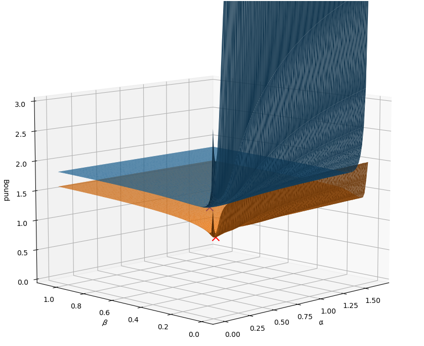
Here, we want to qualitatively analyze the quality of the upper bound, and obtain further insights about their validity. To do so, we used the same setting as our presented ablation studies in Section 4. One advantage is that the scale is small enough that we can directly compare the true PAC-Bayes bound, and the proposed approximation to that bound. However, unlike other experiments, we share and across the layers. This was to meaningfully see the shape of the bound in 3D plots. The results are depicted in Figure 6. Within this experiment, we observe that the true bound (orange) is tighter, but follows qualitatively similar behavior as the proposed approximation (blue). In particular, we find that the optima (orange cross for a true bound, blue cross for approximation) are close to each other. Therefore, we think this data shows the quality of the proposed approximation at a small scale.
F.2 Ablations in the Small-Data Regime
\includestandalone[width=]tikz/appendix/results/results_small_data
tikz/appendix/results/cold_posterior_small
tikz/appendix/results/cold_posterior_large


Next, we extend the ablation studies from Section 4 in order to provide the influence of hyper-parameters namely temperature scaling and weight decays. To achieve this, we keep the same setting as the ablations again and plot for a specified range. Similarly again, as often done in PAC-Bayes literature, we vary the availability of the data and compute the accuracy as a metric. The results can be found in Figure 7. Importantly, this figure shows that the learned prior is in general, more data-efficient. On the other hand, the results also show the conditions when our method is effective. To explain, we observe that for small temperature scaling and large weight decays (top right), the performance of learned prior deteriorates. The results are expected because in the case of large weight decay, the isotropic prior becomes a more dominant term in the learned prior. Thus, the differences become smaller. On the other hand, for a small weight decay, BNNs become closer to deterministic. In that case, learning the prior only helps for small weight decay. Lastly, we find that in a vast range of hyperparameter settings, the learned prior helps to learn more data efficiently, when compared to isotropic priors.
F.3 Further Cold Posterior Experiments
F.3.1 Small-Scale
In Section 4, we presented an empirical result on cold posterior effects. There, we showed that the cold posterior effect is not completely vanished, but is largely mitigated with the proposed learned prior. In this section, we aim to examine the stability of these results w.r.t different weight decay settings. To this end, within the setting of the ablations, we examine variations of three weight decays. The results are shown in Figure 8. In the experiments, we observe similar qualitative behavior, i.e., our learning-based prior largely mitigates the cold posterior effects when compared to the isotropic prior. We also ablate the prior with learned mean, which helps over purely zero mean isotropic Gaussian. Yet, incorporating the curvature, as in our method, improves the results further. Most importantly, our learned prior generates the least deviations due to the changes in the weight decay. Thus, we interpret the results that the learned priors are more stable with respect to changing the weight decay, while better mitigating the cold posterior effects.
F.3.2 Large-Scale
Next, we further examine the cold posteriors within a large scale experiment. To do so, we obtain the posteriors from ImageNet using ResNet-50 architecture and use it as a prior on CIFAR-10. Using CIFAR-10, we then obtain the posterior. We use a learning rate of 1e-3 and a batch size of eight. All other settings are kept the same as in the ablations of Section 4. We do not evaluate the zero mean isotropic prior but only the isotropic prior with the learned mean. This enables direct comparison of the methods, as we only vary the prior. The results are presented in Figure 8. We observe the followings. First, we find that the cold poster effect is strong for the weight decay 1e-3, whereas with the weight decay 1e-5, the learned prior helps. The weight decay of 1e-8 didn’t produce reasonable results for all evaluated temperature scales (up to 1e-15). These results are omitted from the plot for presentation clarity. Finally, the reachable accuracy is higher for the learning-based priors than for the isotropic priors with learned mean, while the influence of random seeds on deviations seems smaller.
F.4 Few-Shot Learning: Results per Data-set
In Section 4, we have presented few-shot learning results, which were averaged across eight data-sets. Now, we present the results per individual data-set. Hence, the results herein is an elaboration to Section 4. Figures 9 and 10 depict the results, four different data-sets each. We observe that in the majority of the data-sets, the learned prior outperforms the isotropic priors as well as the presented baselines, in terms of precision and calibration measures. On the other hand, we also observe that the learned prior cannot uniformly outperform all other baselines across different data-set and metrics. For example, the colorectal histology data-set is one where the isotropic prior outperforms the learned prior, while in oxford pet data-set, the standard BNNs and a deterministic neural network show stronger results in terms of precision and calibration AUC. We think that this is expected, as the prior learning methods assume the existence of relevant data and tasks to learn the prior from. Despite this limitation, as we find that the learned prior more often outperforms the methods based on the isotropic priors, our work shows the relevance of the prior learning methods, i.e., when there exists relevant data and tasks to learn from, there are potential performance advantages over relying on the isotropic priors.