Learning Bayes-Optimal Channel Estimation for Holographic MIMO in Unknown EM Environments
Abstract
Holographic MIMO (HMIMO) has recently been recognized as a promising enabler for future 6G systems through the use of an ultra-massive number of antennas in a compact space to exploit the propagation characteristics of the electromagnetic (EM) channel. Nevertheless, the promised gain of HMIMO could not be fully unleashed without an efficient means to estimate the high-dimensional channel. Bayes-optimal estimators typically necessitate either a large volume of supervised training samples or a priori knowledge of the true channel distribution, which could hardly be available in practice due to the enormous system scale and the complicated EM environments. It is thus important to design a Bayes-optimal estimator for the HMIMO channels in arbitrary and unknown EM environments, free of any supervision or priors. This work proposes a self-supervised minimum mean-square-error (MMSE) channel estimation algorithm based on powerful machine learning tools, i.e., score matching and principal component analysis. The training stage requires only the pilot signals, without knowing the spatial correlation, the ground-truth channels, or the received signal-to-noise-ratio. Simulation results will show that, even being totally self-supervised, the proposed algorithm can still approach the performance of the oracle MMSE method with an extremely low complexity, making it a competitive candidate in practice.
Index Terms:
6G, holographic MIMO, channel estimation, score matching, self-supervised learning, MMSE estimationI Introduction
With an ultra-massive number of antennas closely packed in a compact space, holographic MIMO (HMIMO) is envisioned as a promising next-generation multi-antenna technology that enables extremely high spectral and energy efficiency [2]. To exploit the benefits of the electromagnetic (EM) channel, it is important to acquire accurate channel state information. However, this is difficult owing to both the high dimensionality of the channel and its complicated EM characteristics.
The minimum mean-square-error (MMSE) estimator is able to achieve the Bayes-optimal performance in terms of MSE. Implementing it requires either a perfect knowledge of the prior distribution of the channels [3, 4], or learning such a distribution from a substantial number of ground-truth channels [5, 6], both of which are difficult, if not impossible, in HMIMO systems owing to the extremely large number of antennas. Additionally, the computational complexity of the MMSE estimator, even the linear version (LMMSE), is extremely high, since it involves computationally-intensive matrix inversion operations, which consume a significant amount of computational budget [7]. Existing studies proposed various low-complexity alternatives, but they all come at the cost of an inferior performance compared with the MMSE estimator. In [3], a subspace-based channel estimation algorithm was proposed, in which the low-rank property of the HMIMO spatial correlation was exploited without requiring the full knowledge of the spatial correlation matrix. In [8], a discrete Fourier transform (DFT)-based HMIMO channel estimation algorithm was proposed by approximating the spatial correlation with a suitable circulant matrix. Nevertheless, such an algorithm was limited to uniform linear array (ULA)-based HMIMO systems, and cannot be extended to the more general antenna array geometries. In [4], a concise tutorial on HMIMO channel modeling and estimation was presented. Even though the aforementioned estimators significantly outperform the conventional least squares (LS) scheme, there still exists quite a large gap from that of the MMSE estimator.
In this paper, we affirmatively answer a fundamental question: Is it possible to establish a Bayes-optimal MMSE channel estimator for HMIMO systems in arbitrarily unknown EM environments? Owing to the complicated channel distribution and the ultra-high dimensionality of the problem, classical analytical methods become either sub-optimal in performance or too complicated to implement. Supervised deep learning-based methods can achieve near-optimal performance, but highly rely on a substantial dataset of the ground-truth channels [5], which is difficult to achieve in HMIMO systems. The data availability and complexity constitute the two core challenges that prevents the practical implementation of the MMSE channel estimator in HMIMO systems. These challenges can be both tackled by our proposed learning-based estimator:
-
1.
Data availability: The proposed estimator needs neither the prior distribution nor the ground-truth channel data. Only the received pilot signals are required at the model training stage.
-
2.
Complexity: The proposed estimator drops the prohibitive matrix inversion, and is with extremely low complexity.
Specifically, we propose a self-supervised deep learning framework for realizing the Bayes-optimal MMSE channel estimator for HMIMO. We first prove in theory that the MMSE channel estimator could be constructed based solely on the distribution of the received pilot signals through the Stein’s score function. Afterwards, we propose a practical algorithm to train neural networks to estimate the score function solely by using the collected received pilot signals. Lastly, a low-complexity principal component analysis (PCA)-based method is proposed to estimate the received signal-to-noise-ratio (SNR) from pilots alone, since it is required in the score-based MMSE estimator. Simulation results in both isotropic and non-isotropic environments are provided to illustrate the effectiveness and efficiency of the proposed estimator. Notably, it achieves almost the same performance as the oracle MMSE estimator with more than 20 times reduction in complexity, in a nominal HMIMO setup.
Notation: is a scalar. is the -norm of a vector . , , , are the transpose, Hermitian, the real part, and the imaginary part of a matrix , respectively. and are complex and real Gaussian distributions with mean and covariance , respectively. is an identity matrix with an appropriate shape.
II HMIMO System and Channel Models
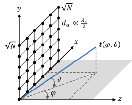
Consider the uplink of an HMIMO system, where the base station (BS) is equipped with a uniform planar array (UPA) with antennas that simultaneously serves single antenna-user equipments (UEs). We focus on the cases where the BS has thousands of closely packed antennas with spacings below the nominal value of half the carrier wavelength . We define a local spherical coordinate system at the UPA with and being the azimuth and elevation angles of arrival (AoAs), respectively, as depicted in Fig. 1. We index the antennas row-by-row with , and denote the position of the -th antenna as , in which
| (1) |
The notations and refer to the modulus operation and the floor function, respectively. Considering a planar wave impinging on the UPA111While we focus on the far-field case here, our proposal is also applicable to the near-field case [9], which will be discussed in our follow-up works. , the array response vector is given by
| (2) |
with being the unit vector in the AoA direction. We assume that orthogonal pilots are adopted and consider the channel between the BS and an arbitrary UE, consisting of the superposition of multi-path components that can be represented by a continuum of planar waves [3], given by
| (3) |
where denotes the angular spread function specifying the phase shift and the gain for each AoA direction . In accordance with [3], we can model as a spatially uncorrelated symmetric Gaussian stochastic process with cross-correlation given by
| (4) |
where is the average channel gain, denotes the Dirac delta function, and is the spatial scattering function, i.e., the joint probability density function (PDF) of the azimuth and elevation AoAs. The function is normalized such that . The HMIMO channel can be modeled by the correlated Rayleigh fading222Notice that the proposed algorithm can work with any possible distribution of the HMIMO channel. We follow the convention in the literature and adopt the correlated Rayleigh fading here. This is because in this case, the Bayes-optimal estimator admits a closed form if the covariance is perfectly known, which can serve as the oracle performance bound to benchmark our algorithm. , i.e., , with a spatial correlation matrix , which satisfies [3, 8]. Following (4), the correlation matrix can be calculated by
| (5) |
For any function , the -th entry of the correlation matrix is given by
| (6) |
where denotes the -th element of a matrix. While in most cases the integral in (6) could only be computed numerically, a closed form solution exists in isotropic scattering environments, where the covariance is given in [10] as
| (7) |
Here denotes the sinc function, while is the Euclidean norm. In non-isotropic scattering environments where the augular density is not evenly distributed in the whole space, takes many distinct forms in the literature. For example, in [3], the non-isotropic scattering function is assumed to follow a cosine directivity pattern, while in [4], the leading eigenvalues of are truncated to obtain a non-isotropic covariance, which will be detailed in Section IV.
We then introduce the system model. In the uplink channel estimation phase, the UEs send known pilot sequences to the BS. Assuming that the orthogonal pilots are utilized, the real-valued equivalent of the received pilot signal (measurement) from an arbitrary UE, , is given by333Similar to [3], we consider a fully-digital system model, in which the dimensions of and are identical. Nevertheless, the proposed algorithm can be readily extended to compressed sensing-based channel estimation in hybrid analog-digital systems, in a similar manner as [11].
| (8) |
where represents the real-valued channel, is the received signal-to-noise-ratio (SNR), and is the additive white Gaussian noise. The channel estimator, in practice, should only have the knowledge of , without knowing the true covariance or the SNR .
III MMSE Estimation via Score Matching
In the following, we first discuss how to derive the score-based MMSE estimator solely based on the received pilots , and then introduce how to estimate the two key components of the algorithm, i.e., the score function and the received SNR.
III-A Bridging MMSE Estimation with the Score Function
Our target is a Bayes-optimal channel estimator, , that minimizes the mean-square-error (MSE), i.e.,
| (9) |
where the expectation above is taken with respect to (w.r.t.) the unknown channel , while is the posterior density. Taking a derivative of the above equation w.r.t. and nulling it, we reach the Bayes-optimal, i.e., minimum MSE (MMSE), channel estimator, given by
| (10) |
where is the joint density, and is the measurement density obtained via marginalization, i.e.,
| (11) | ||||
The last equality holds since the likelihood function expresses as a convolution between the prior distribution and the i.i.d. Gaussian noise. Taking the derivative of both sides of (11) w.r.t. gives
| (12) | ||||
Dividing both sides of (12) w.r.t. results in the following:
| (13) | ||||
where the second equality holds owing to the Bayes’ theorem, and the last equality holds due to (10) and . By rearranging the terms and plugging in , we reach the foundation of the proposed algorithm:
| (14) |
where is called the Stein’s score function in statistics [12]. From (14), we notice that the Bayes-optimal MMSE channel estimator can be achieved solely based on the received pilot signals , without access to the prior distribution or a supervised dataset of the ground-truth channels , which are unavailable in practice. With an efficient estimator of the score function , the Bayes-optimal MMSE channel estimator can be computed in a closed form with extremely low complexity. In addition, since (14) holds regardless of the distribution of the HMIMO channel , one can construct the MMSE estimator in arbitrary EM environments without any assumptions on the scatterers or the array geometry.
It is noticed that two terms that should be obtained in (14), i.e., the received SNR and the measurement score function . In the following, we discuss on how to utilize machine learning tools to obtain an accurate estimation of them based solely on the measurement .
III-B Self-Supervised Learning of the Score Function
We discuss how to get the score function . Given that a closed-form expression is intractable to acquire, we instead aim to achieve a parameterized function with a neural network, and discuss how to train it based on score matching. We first introduce the denoising auto-encoder (DAE) [12], the core of the training process, and explain how to utilize it to approximate the score function.
To obtain the score function , the measurement is treated as the target signal that the DAE should denoise. The general idea is to obtain the score function based on its analytical relationship with the DAE of , which will be established later in Theorem 1. We first construct a noisy version of the target signal by manually adding some additive white Gaussian noise, , where and controls the noise level444Note that the extra noise is only added during the training process. , and then train a DAE to denoise the manually added noise. The DAE, denoted by , is trained by the -loss function, i.e.,
| (15) |
The theorem below explains the relationship between the score function and the trained DAE.
Theorem 1 (Alain-Bengio [12, Theorem 1]).
The optimal DAE, , behaves asymptotically as
| (16) |
Proof:
Please refer to [12, Appendix A]. ∎
The above theorem indicates that, for a sufficiently small , we can approximate the score function based on the DAE by , assuming that parameter of the DAE, , is near-optimal, i.e., . Nevertheless, the approximation can be numerically unstable as the denominator, , is close to zero. To alleviate the problem, we improve the structure of the DAE and rescale the original loss function.
First, we consider a residual form of the DAE with a scaling factor. Specifically, let . Plugging it into (16), the score function is approximately equal to
| (17) |
when holds. This reparameterization enables to approximate the score function directly, thereby circumventing the need for division that may lead to numerical instability. Also, the residual link significantly enhances the capability of the DAE, since it can easily learn an identity mapping [13].
Second, since the variance of the manually added noise is small, the gradient of the DAE loss function (15) can easily vanish to zero and may lead to difficulties in training. Hence, we rescale the loss function by a factor of to safeguard the vanishing gradient problem, i.e.,
| (18) |
where (17) is plugged into the loss function.
We are interested in the region where is sufficiently close to zero, in which case can be deemed to be equal to the score function according to (17). Nevertheless, directly training the network using a very small is difficult since the SNR of the gradient signal decreases in a linear rate with respect to , which introduces difficulty for the stochastic gradient descent [14]. To exploit the asymptotic optimality of the score function approximation when , we propose to simultaneously train the network with varying values, to handle various levels and then naturally generalize to the desired region, i.e., . To achieve the goal, we control the manually added noise by letting follow a zero-mean Gaussian distribution and gradually anneal from a large value to a small one in each iteration. That is, we condition on the manually added noise level during training.
The proposed algorithm is shown in Algorithm 1. The DAE is trained using stochastic gradient descent for epochs. In each epoch, we draw a random vector and anneal in to control the extra noise level according to the current number of iterations . Then, the DAE loss function in (18) is minimized by stochastic optimization. Note that in the training process, nothing but a dataset of the received pilot signals is necessary, which is readily available in practice. In the inference stage, one can apply formula (14) to compute the score-based MMSE estimator, in which the score function can be approximated by using , i.e., setting as zero, and the received SNR can be estimated by the PCA-based algorithm in the next subsection.
For the neural architecture of the DAE , we adopt a simplified UNet architecture [15]. Note that depending on the complexity budget, many other prevailing neural architectures could also be applied [6]. Other details of the training process are deferred to Section IV.
III-C PCA-Based Received SNR Estimation
We propose a low-complexity PCA-based algorithm to estimate the received SNR in (14) based on a single instance of the pilot signals . Before further discussion, we stress that the received SNR estimation is executed only at the inference stage, not at the training stage, as shown in Algorithm 1.
The basic idea behind the PCA-based algorithm is the low-rankness of the spatial correlation matrix of HMIMO due to the dense deployment of the antenna elements. Specifically, for isotropic scattering environments, the rank of the correlation matrix is approximately [17]. It decreases with the shrink of antenna spacing and the increase of the carrier frequency. For example, when , around of the eigenvalues of shrinks towards zero. The rank deficiency of tends to be even more prominent in the case of non-isotropic scattering environments [4].
Similar to Fig. 2 in our previous work [16], we decompose multiple virtual subarray channels (VSCs) from the HMIMO channel by a sliding window. Specifically, we reshape the real-valued HMIMO channel into a tensor form . We then decompose into VSC tensors using a sliding window of size , and then reshape them back into the vector form to obtain a set of VSCs, denoted by . Similarly, the received pilot signals and the noise could also be decomposed as and , and should satisfy
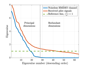
| (19) |
Due to the low-rankness of the spatial correlation matrix , the decomposed VSCs should also lie in a low-dimensional subspace. In Fig. 2, we plot the eigenvalues of the covariance matrices of the decomposed VSCs from an HMIMO channel in isotropic scattering environments and their corresponding received pilots , respectively, with a reference line marking the inverse of the received SNR . According to the figure, the eigenvalues of the covariance of quickly shrinks to zero with about 30 principal dimensions. The zero eigenvalues correspond to the redundant dimensions. In contrast, we observe that the eigenvalues of the covariance of are concentrated around in the redundant dimensions. This example suggests that it is indeed possible to estimate the received SNR based on the redundant eigenvalues. Rigorously, these eigenvalues could be proved to follow a Gaussian distribution [16]. Plus, the principal and redundant eigenvalues could be separated by an iterative process. Hence, we could leverage [16, Algorithm 1] to accurately estimate the received SNR. Detailed setups are discussed in Section IV.
III-D Complexity Analysis
The inference complexity of the proposed algorithm consists of the computation of and the PCA-based estimation of . The former depends upon the specific neural architecture of , and costs a constant complexity, denoted by , once the network is trained. The computational complexity for the latter, as analyzed in [16], is given by , where , the size of the sliding window, is usually quite small. Hence, the overall complexity is , which scales only linearly with respect to the number of antennas .
In practice, the fluctuation of the received SNR may not be frequent. In such a case, it is not a necessity to estimate the received SNR for every instance of the received pilot signals . Therefore, the actual complexity of the proposed score-based algorithm is within the range of and , which is extremely efficient given near-optimal performance555Most previous works on channel estimation assume that the received SNR is perfectly known. In this case, the complexity reduces to . . By sharp contrast, the (oracle) MMSE estimator requires time-consuming matrix inversion, which is as complex as . In Section IV, we provide a running time complexity to offer a straightforward comparison.
IV Simulation Results
IV-A Simulation Setups
We consider a typical HMIMO system setup with and . In the training stage, the hyper-parameters of the proposed score-based algorithm are chosen as , , , , and . Also, the learning rate is decayed by half after every 25 epochs. In the inference stage, the size of the sliding window is set as . The performance discussed below is all averaged over a held-out dataset consisting of testing samples.
| / (SNR) | Method | Bias | Std | RMSE |
|---|---|---|---|---|
| 1.0000 (0 dB) | Oracle | 0.0004 | 0.0160 | 0.0160 |
| Proposed | 0.0080 | 0.0371 | 0.0380 | |
| Sparsity | 0.1769 | 0.0277 | 0.1790 | |
| 0.1778 (15 dB) | Oracle | <0.0001 | 0.0028 | 0.0028 |
| Proposed | 0.0031 | 0.0064 | 0.0071 | |
| Sparsity | 0.1530 | 0.0163 | 0.1539 |
For isotropic scattering, the covariance is given via (7). In the non-isotropic case, we follow [4] and also construct the covariance by truncating the leading eigenvalues of . Mathematically, the non-isotropic covariance could be expressed as , where is a matrix consisting of the eigenvectors of , while is a diagonal matrix that contains the eigenvalues of arranged in descending order. To truncate the matrix, we select only the first eigenvalues and eigenvectors of .
IV-B Accuracy of Received SNR Estimation
The accuracy of the received SNR estimation can influence the performance of the proposed score-based estimator. Hence, different from previous works that assume perfect knowledge of the received SNR, we propose a practical PCA-based means to estimate it and examine its performance. In Table I, we list the estimation accuracy under different SNRs. We present the performance in terms of the inverse of the SNR, i.e., , since it is used in (14). The bias, the standard deviation (std), and the root MSE (RMSE) are given by , , and , respectively. The estimator’s accuracy and robustness are reflected with the bias and std, while the RMSE provides an assessment of its overall performance. From Table I, we observe that the performance of the proposed PCA-based method is both highly accurate and robust, and outperforms the sparsity-based median absolute deviation (MAD) estimator in [18], as HMIMO channels are not exactly sparse. Also, the performance is close to the oracle bound which assumes perfect knowledge of the channel , and estimate directly from [16]. Later, in Section IV-D, we will illustrate that the proposed score-based channel estimator is robust to SNR estimation errors.
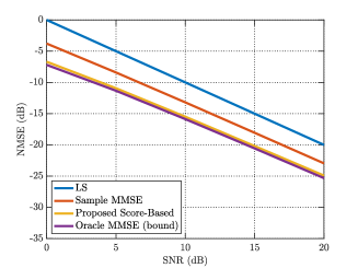
IV-C Normalized MSE (NMSE) in Isotropic and Non-Isotropic Scattering Environments
We compare the proposed score-based estimator with three benchmarks, including LS, sample MMSE, and oracle MMSE. Here, oracle MMSE refers to the MMSE estimator with perfect knowledge of both the covariance and the received SNR , which is the Bayesian performance bound, given by
| (20) |
This is difficult, if not impossible, to acquire in practice since contains entries and is prohibitive to estimate when is particularly large in an HMIMO system. The sample MMSE method utilizes the same equation as (20), but replaces the true covariance with an estimated one based upon the testing samples, given by [8], where is the number of testing samples and denotes the -th sample of the received pilot signals in the testing dataset. We also utilize the perfect received SNR in sample MMSE.
In Fig. 3(a), we present the NMSE as a function of the SNR in isotropic scattering environments. It is illustrated that the proposed score-based algorithm significantly outperforms the LS and the sample MMSE estimator, and achieves almost the same NMSE as the oracle MMSE bound at every SNR level. Note that the oracle MMSE method utilizes the true covariance and received SNR, but the proposed method requires neither.
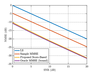
In Fig. 3(b), we compare the NMSE in non-isotropic environments, in which the rank of the covariance matrix is further reduced. As a result, the performance gap between the LS and the oracle MMSE estimator is enlarged as the rank deficiency becomes more significant. Nevertheless, similar to the isotropic case, the proposed score-based estimator exhibits almost the same performance as the oracle bound and significantly outperforms the sample MMSE method, illustrating its effectiveness in different scattering environments.
IV-D Robustness to SNR Estimation Errors
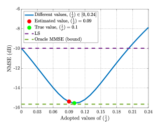
In Fig. 3(c), we provide discussions on how the accuracy for the received SNR estimation will influence the performance of the proposed score-based estimator. In the simulations, the true value of the received SNR is set as 10 dB, i.e., . We vary the adopted values of in (14) within , and plot the corresponding NMSE performance curve in blue. Particularly, we utilize red and green dots to denote the NMSE achieved with the estimated and true SNR values, respectively. The LS and the oracle MMSE algorithms are presented as the performance upper and lower bounds. It is observed that even when an inexact received SNR is adopted, the performance of the score-based algorithm is still quite robust and significantly outperforms the LS method. Also, the estimated received SNR by the PCA-based method is accurate enough to offer a near-optimal performance, even in unknown EM environments.
IV-E Running Time Complexity
We introduce the CPU running time of the proposed algorithm. For the considered setups, the proposed score-based estimator takes as low as 3 ms on an Intel Core i7-9750H CPU, which is much shorter than that of the oracle MMSE method involving high-dimensional matrix inverse (requiring around 70 ms). The high efficiency and the Bayes-optimal performance in unknown EM environments thus make the proposed score-based algorithm an ideal candidate in practice.
V Conclusion and Future Directions
In this paper, we studied channel estimation for the HMIMO systems, and proposed a score-based MMSE channel estimator that can achieve Bayes-optimal performance with an extremely low complexity. Particularly, the proposed algorithm is trained solely based on the received pilots, without requiring any kind of priors or supervised datasets that are prohibitive to collect in practice. This enables it to work in arbitrary and unknown EM environments that may appear in real-world deployment. As a future direction, it is interesting to extend to the proposed framework to compressed sensing-based setups. Furthermore, since the proposed algorithm is self-supervised, it is promising to investigate the possibility of online learning and adaptation.
References
- [1] W. Yu, H. He, X. Yu, S. Song, J. Zhang, R. D. Murch, and K. B. Letaief, “Bayes-optimal unsupervised learning for channel estimation in near-field holographic MIMO,” arXiv preprint arXiv:2312.10438, 2023.
- [2] A. Pizzo, T. L. Marzetta, and L. Sanguinetti, “Spatially-stationary model for holographic MIMO small-scale fading,” IEEE J. Sel. Areas Commun., vol. 38, no. 9, pp. 1964–1979, Sept. 2020.
- [3] O. T. Demir, E. Bjornson, and L. Sanguinetti, “Channel modeling and channel estimation for holographic massive MIMO with planar arrays,” IEEE Wireless Commun. Lett., vol. 11, no. 5, pp. 997–1001, May 2022.
- [4] J. An, C. Yuen, C. Huang, M. Debbah, H. V. Poor, and L. Hanzo, “A tutorial on holographic MIMO communications–part I: Channel modeling and channel estimation,” IEEE Commun. Lett., vol. 27, no. 7, pp. 1664–1668, Jul. 2023.
- [5] W. Yu, Y. Shen, H. He, X. Yu, S. Song, J. Zhang, and K. B. Letaief, “An adaptive and robust deep learning framework for THz ultra-massive MIMO channel estimation,” IEEE J. Sel. Topics Signal Process., vol. 17, no. 4, pp. 761–776, Jul. 2023.
- [6] W. Yu, Y. Ma, H. He, S. Song, J. Zhang, and K. B. Letaief, “AI-native transceiver design for near-field ultra-massive MIMO: Principles and techniques,” arXiv preprint arXiv:2309.09575, 2023.
- [7] H. He, C.-K. Wen, S. Jin, and G. Y. Li, “Model-driven deep learning for MIMO detection,” IEEE Trans. Signal Process., vol. 68, pp. 1702–1715, Feb. 2020.
- [8] A. A. D’Amico, G. Bacci, and L. Sanguinetti, “DFT-based channel estimation for holographic MIMO,” in Proc. Asilomar Conf. Signals Syst. Comput., Pacific Grove, CA, USA, Nov. 2023.
- [9] Z. Wang, J. Zhang, H. Du, D. Niyato, S. Cui, B. Ai, M. Debbah, K. B. Letaief, and H. V. Poor, “A tutorial on extremely large-scale MIMO for 6G: Fundamentals, signal processing, and applications,” arXiv preprint arXiv:2307.07340, 2023.
- [10] A. de Jesus Torres, L. Sanguinetti, and E. Bjornson, “Electromagnetic interference in RIS-aided communications,” IEEE Wireless Commun. Lett., vol. 11, no. 4, pp. 668–672, Apr. 2022.
- [11] C. A. Metzler, A. Maleki, and R. G. Baraniuk, “From denoising to compressed sensing,” IEEE Trans. Inf. Theory, vol. 62, no. 9, pp. 5117–5144, Sept. 2016.
- [12] G. Alain and Y. Bengio, “What regularized auto-encoders learn from the data-generating distribution,” J. Mach. Learn. Res., vol. 15, no. 1, pp. 3563–3593, Nov. 2014.
- [13] K. He, X. Zhang, S. Ren, and J. Sun, “Deep residual learning for image recognition,” in Proc. IEEE Conf. Comput. Vis. Pattern Recog., Las Vegas, NV, USA, Jun. 2016.
- [14] J. H. Lim, A. Courville, C. Pal, and C.-W. Huang, “AR-DAE: towards unbiased neural entropy gradient estimation,” in Proc. Int. Conf. Mach. Learn., Virtual, Jul. 2020.
- [15] O. Ronneberger, P. Fischer, and T. Brox, “U-net: Convolutional networks for biomedical image segmentation,” in Proc. Int. Conf. Med. Image Comput. Comput.-Assisted Intervention, Munich, Germany, Oct. 2015.
- [16] W. Yu, H. He, X. Yu, S. Song, J. Zhang, and K. B. Letaief, “Blind performance prediction for deep learning based ultra-massive MIMO channel estimation,” in Proc. IEEE Int. Conf. Commun., Rome, Italy, May 2023.
- [17] A. Pizzo, L. Sanguinetti, and T. L. Marzetta, “Fourier plane-wave series expansion for holographic MIMO communications,” IEEE Trans. Wireless Commun., vol. 21, no. 9, pp. 6890–6905, Sept. 2022.
- [18] A. Gallyas-Sanhueza and C. Studer, “Low-complexity blind parameter estimation in wireless systems with noisy sparse signals,” IEEE Trans. Wireless Commun., vol. 22, no. 10, pp. 7055–7071, Oct. 2023.