Learning Approximate Forward Reachable Sets
Using Separating Kernels
Abstract
We present a data-driven method for computing approximate forward reachable sets using separating kernels in a reproducing kernel Hilbert space. We frame the problem as a support estimation problem, and learn a classifier of the support as an element in a reproducing kernel Hilbert space using a data-driven approach. Kernel methods provide a computationally efficient representation for the classifier that is the solution to a regularized least squares problem. The solution converges almost surely as the sample size increases, and admits known finite sample bounds. This approach is applicable to stochastic systems with arbitrary disturbances and neural network verification problems by treating the network as a dynamical system, or by considering neural network controllers as part of a closed-loop system. We present our technique on several examples, including a spacecraft rendezvous and docking problem, and two nonlinear system benchmarks with neural network controllers.
keywords:
Stochastic reachability, kernel methods, neural network verification1 Introduction
Reachability analysis is important in many dynamical systems for its ability to provide assurances of desired behavior, such as reaching a desired target set or anticipating potential intersection with a set known to be unsafe. Such analysis has shown utility in a variety of safety-critical applications, including autonomous cars, UAVs, and spacecraft. The forward stochastic reachable set describes the set of states that the system will reach with a non-zero likelihood. While most approaches for stochastic reachability are model-based, data-driven approaches are important when mathematical models may not exist or may be too complex for existing numerical approaches. In particular, the growing presence of learning-enabled components in dynamical systems warrants the development of new tools for stochastic reachability that can accommodate neural networks, look-up tables, and other model-resistant elements. In this paper, we propose a technique for data-driven stochastic reachability analysis that provides a convergent approximation to the true stochastic reachable set.
Significant advances have been made in verification of dynamical systems with neural network components. Recent work in Seidman et al. (2020); Weinan (2017) has shown that neural networks can be modeled as a nonlinear dynamical system, making them amenable in some cases to model-based reachability analysis. Typically, these approaches presume that the neural network exhibits a particular structure, such as having a particular activation function, as in Sidrane and Kochenderfer (2019); Tran et al. (2020), and exploit existing tools for forward reachability, such as Althoff (2015); Chen et al. (2013). Other approaches employ a mixed integer linear programming approach, as in Dutta et al. (2017, 2019); Lomuscio and Maganti (2017). These techniques exploit Lipschitz constants or perform set propagation, however, the latter approach becomes intractable for large-scale systems due to vertex facet enumeration. Further, in practice, knowledge of the network structure or dynamics may not be available, or may be too complex to use with standard reachability methods. Thus, additional tools are needed to efficiently compute stochastic reachable sets.
Data-driven reachability methods provide convergent approximations of reachable sets with high confidence, but are typically unable to provide assured over-approximations. Methods have been developed that use convex hulls in Lew and Pavone (2020) and scenario optimization in Devonport and Arcak (2020). However, these approaches rely upon convexity assumptions which can be limiting in certain cases. Other data-driven approaches leverage a class of machine learning techniques known as kernel methods, including Gaussian processes in Devonport and Arcak (2020) and support vector machines in Allen et al. (2014); Rasmussen et al. (2017). However, the approach in Rasmussen et al. (2017) can suffer from stability issues and does not provide probabilistic guarantees of convergence, and the approach in Allen et al. (2014) requires that we repeatedly solve a nonlinear program offline to generate data for the SVM classifier. The approach in Devonport and Arcak (2020) requires use of a Gaussian process prior. In contrast to these approaches, we propose a method that can accommodate nonlinear dynamical systems with arbitrary stochastic disturbances.
Our approach employs a class of kernel methods known as separating kernels to form a reachable set classifier. By learning a set classifier in Hilbert space, we convert the problem of learning a set boundary into the problem of learning a classifier in a high-dimensional space of functions. Our approach extends the work in De Vito et al. (2014) to the problem of learning reachable sets for stochastic systems that overcomes the stability and convergence issues faced by existing kernel based approaches and allows for arbitrary stochastic disturbances. Our main contribution is an application of the techniques presented in De Vito et al. (2014) to the problem of learning approximate forward reachable sets and neural network verification. Similar to other data-driven approaches, the approximation proposed here does not provide guarantees in the form of assured over- or under-approximations of the forward reachable set. However, although empirically derived, the approximation can be shown to converge in probability almost surely.
The paper is structured as follows: Section 2 formulates the problem. We describe the application of kernel methods to compute approximate forward reachable sets in Section 3, and discuss their convergence properties and finite sample bounds. In Section 4, we demonstrate our approach on a realistic satellite rendezvous and docking problem, as well as two neural network verification benchmarks from Dutta et al. (2019). Concluding remarks are presented in Section 5.
2 Problem Formulation
We use the following notation throughout: Let be an arbitrary nonempty space, and denote the -algebra on by . Let denote the set of all subsets (the power set) of . If is a topological space (Çinlar, 2011), the -algebra generated by the set of all open subsets of is called the Borel -algebra, denoted by . If is countable, with -algebra , then it is called discrete. Let denote a probability space, where is the -algebra on and is a probability measure on the measurable space . A measurable function is called a random variable taking values in . The image of under , , is called the distribution of . Let be an arbitrary set, and for each , let be a random variable. The collection of random variables on is a stochastic process.
2.1 System Model
Consider a general discrete-time system with dynamics given by:
| (1) |
with state , input , parameters , and stochastic process , comprised of the random variables , , defined on the measurable space , . The system evolves over a finite time horizon from initial condition , which may be chosen according to initial probability measure . We assume that the dynamics and the structure of the disturbance are unknown, but that a finite sample of observations, , taken i.i.d. from , are available.
A special case of this formulation is a feedforward neural network (Seidman et al., 2020; Weinan, 2017), where denotes the layer of the network, are the network parameters, and the dimensionality of the state, input, parameter, and disturbance spaces depends on and can change at each layer. For example, in each layer, , where is a map to and is the dimensionality of the state at each layer.
2.2 Forward Reachable Set
Consider a discrete time stochastic system (1). We consider an initial condition and evolve (1) to compute the forward reachable set, . Formally, we define the forward reachable set as in Lew and Pavone (2020), which is a modification of the definition in Mitchell (2007) or Rosolia and Borrelli (2019) that is amenable to neural network verification problems.
Definition 2.1 (Lew and Pavone, 2020).
Given an initial condition , the forward reachable set is defined as the set of all possible future states at time for a system following a given control sequence .
| (2) |
Note that is a random variable on the probability space , and that the forward reachable set can also be viewed as the support of (Vinod et al., 2017), which is the smallest closed set such that .
We seek to compute an approximation of the forward reachable set in (2) for a system (1) with unknown dynamics, by using the theory of reproducing kernel Hilbert spaces. We formulate the problem as learning a classifier function in Hilbert space which describes the geometry of the forward reachable set boundary. We presume that the forward reachable set (2) is implicitly defined by the classifier .
| (3) |
Hence, we seek to compute an empirical estimate of in (3) using observations taken from the system evolution .
Forward reachability often focuses on forming an over-approximation that is a superset of . However, because our proposed approach cannot provide such a guarantee, we aim to provide an approximation of the forward reachable set by computing that is convergent in probability almost surely. These probabilistic guarantees are important to ensure the consistency of our result and that our estimated classifier (and therefore the approximate reachable set) is close to the true result with high probability. The main difficulty in this problem arises from the fact that we do not have explicit knowledge of the dynamics (1) or place any prior assumptions on the structure of the uncertainty. This makes the proposed method a useful technique in the context of existing stochastic reachability toolsets, since it can be used on black-box systems with arbitrary disturbances. Note that because we seek to estimate a classifier , in contrast to existing approaches that employ polytopic methods, our approach does not provide a simple geometric representation.
3 Finding Forward Reachable Sets Using Separating Kernels
Let denote the Hilbert space of real-valued functions on equipped with the inner product and the induced norm .
Definition 3.1 (Aronszajn, 1950).
A Hilbert space is a reproducing kernel Hilbert space if there exists a positive definite kernel function that satisfies the following properties:
| (4a) | |||||
| (4b) | |||||
where (4b) is called the reproducing property, and for any , we denote in the RKHS as a function on such that .
Alternatively, by the Moore-Aronszajn theorem (Aronszajn, 1950), for any positive definite kernel function , there exists a unique RKHS with as its reproducing kernel, where is the closure of the linear span of functions . In other words, the Moore-Aronszajn theorem allows us to define a kernel function and obtain a corresponding RKHS.
Let be the reproducing kernel function for the RKHS on . We stipulate that the kernel also satisfies the conditions for being a completely separating kernel. This property ensures that the kernel function can be used to learn the support of any probability measure on . We induce a metric on via the kernel function ,
| (5) |
which is known as the kernel-induced metric on , and is equivalent to the Euclidean metric if is completely separating and continuous. Following De Vito et al. (2014), we define the notion of separating a subset .
Theorem 3.2 (De Vito et al., 2014, Theorem 1).
An RKHS separates a subset if for all , there exists such that and for all . In this case we also say that the corresponding reproducing kernel separates .
According to Theorem 3.2, we need to determine the existence of a function in that acts as a classifier for a subset . Since the functions have the form , this amounts to choosing a kernel function which exhibits the separating property. Note that not all kernel functions can separate every subset . In order to ensure that this is possible, the notion of completely separating kernels is defined.
Definition 3.3 (De Vito et al., 2014, Definition 2).
A reproducing kernel Hilbert space satisfying the assumption that for all with we have is called completely separating if separates all the subsets which are closed with respect to the metric . In this case, we also say that the corresponding reproducing kernel is completely separating.
For example, with , the Abel kernel , where , is a completely separating kernel function (De Vito et al., 2014, Proposition 5). Thus, by properly selecting the kernel function , we ensure that we can classify any subset .
We now turn to a discussion of the classifier in (3). The following theorems are reproduced with modifications for simplicity from De Vito et al. (2014), and ensure we can define as the support of , and that (3) holds.
Proposition 3.4 (De Vito et al., 2014, Proposition 2).
Assume that for all with , , the RKHS with kernel is separable, and is measurable with respect to the product -algebra . There exists a unique closed subset with satisfying the following property: if is a closed subset of and then .
For any subset , let denote the closure of the linear span of functions , and define as the orthogonal projection onto the closed subspace . Define the function such that . Using this definition, we can now define the support in terms of a function .
Theorem 3.5 (De Vito et al., 2014, Theorem 3).
Under the assumptions of Proposition 3.4 and the assumption that for all , if separates the support of the measure , then .
Thus, we aim to learn the forward reachable set (3) by identifying a function that separates the support in .
3.1 Estimating Forward Reachable Sets
The classifier is an element of the RKHS , meaning it has the form and admits a representation in terms of the finite support , , given by:
| (6) |
where are coefficients that depend on . Let be a sample of terminal states at time taken i.i.d. from the system evolution. We seek an approximation of the forward reachable set in (3) using . Thus, we form an estimate of using the form in (6) with data . We can view the estimate as the solution to a regularized least-squares problem.
| (7) |
where is the regularization parameter. The solution to (7) is unique and admits a closed-form solution, given by:
| (8) |
where is called a feature vector, with elements , and is known as the Gram matrix, with elements . A point is estimated to belong to the support of if , where is a threshold parameter that depends on the sample size . Thus, we form an approximation of the forward reachable set in (3) as:
| (9) |
Using this representation, we obtain an estimator which can be used to determine if a point is in the approximate forward reachable set .
3.2 Convergence
We characterize the conditions for the convergence of the empirical forward reachable set to via the Hausdorff distance. We assume that is a topological metric space with metric .
Definition 3.6 (Hausdorff Distance).
Let be nonempty subsets of the metric space . The Hausdorff distance between sets and is defined as
| (10) |
where denotes the set of all points in within a ball of radius around .
The Hausdorff distance gives us a method to measure convergence of the estimate to the true reachable set . In fact, almost surely under mild conditions on the regularization and threshold parameters, and (De Vito et al., 2014, Theorem 6). As the sample size increases, if is chosen according to:
| (11) |
and under the condition that , the empirical forward reachable set converges in probability almost surely to the true forward reachable set .
Furthermore, De Vito et al. (2014, Theorem 7) shows that the approximation admits finite sample bounds on the error of the estimated classifier function. Let be the integral operator with kernel . If with , where denotes the pseudo-inverse of , and the eigenvalues of satisfy for some (see Caponnetto and De Vito, 2007, Proposition 3), then for and , if and is a suitable constant, then
| (12) |
with probability . These guarantees ensure the accuracy of our results in a probabilistic sense, meaning that by increasing the sample size , the estimate will approach the true result, and that for a finite sample size , our result is close to the true result with high probability.
As a final remark, we note that although the formulation in (3) is extensible to level set estimation, which involves learning a set with , the convergence of to does not imply that the approximate level sets converge to the true level sets. This requires further analysis that is beyond the scope of the current work.
4 Numerical Results
For all examples, we choose an Abel kernel , . We chose the parameters to be , according to (11), and , where is the sample size used to construct the classifier. As noted in De Vito et al. (2014), can be chosen via cross-validation and we require that be chosen such that . Numerical experiments were performed in Matlab on an AWS cloud computing instance, and computation times were obtained using Matlab’s Performance Testing Framework. Code to reproduce the analysis and all figures is available at: \urlhttps://github.com/unm-hscl/ajthor-ortiz-L4DC2021
4.1 Clohessy-Wiltshire-Hill System

We first consider a realistic example of spacecraft rendezvous and docking to compare our technique against a known result. The dynamics of a CWH system are defined in Lesser et al. (2013) as:
| (13) | ||||
with state , input , where , and parameters , . We first discretize the dynamics in time and then apply an affine Gaussian disturbance , which is a stochastic process defined on with variance such that .
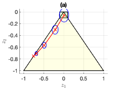
With initial condition , we compute an open-loop control policy using a chance-constrained algorithm from Vinod and Oishi (2019) implemented in SReachTools (Vinod et al., 2019). The control policy is designed to dock with another spacecraft while remaining within a line of sight cone. We then simulated trajectories to collect a sample consisting of the resulting terminal states . A classifier was then computed using (8). In order to depict the sets graphically, we then chose a small region around the mean of the observed state values and computed a visual representation of the forward reachable set by sampling 10,000 points uniformly over the region and connecting evaluations where along the set boundary.
Figure 1 compares the computed approximate forward reachable sets to forward reachable sets computed using the known Gaussian disturbance properties. We can see that the approximate forward reachable sets in Figure 1(a) are close to the variance ellipses produced from the known disturbance properties in 1(b), demonstrating that our approach provides a good estimate of the support of the underlying distribution. Computation time for the approximate forward reachable sets was 1.582 seconds using the kernel based approach. This technique could be accelerated with approximative speedup techniques that are common to kernel methods, such as random Fourier features (Rahimi and Recht, 2008) or FastFood (Le et al., 2013). Additionally, incorporating active or adversarial sampling, as in Lew and Pavone (2020), could reduce computation time by reducing the number of observations needed to compute the classifier.
4.2 Neural Network Verification
We now demonstrate our approach on a set of dynamical system benchmarks with neural network controllers as described in Dutta et al. (2019). We define a feed-forward neural network controller as , with activation functions , that depend on the parameters . The function maps the states into the first layer, and is a function that maps the output of the last layer into the control space. After generating observations of the states, we then assume no knowledge of the structure of or the dynamics.
4.2.1 TORA Model


Consider a translational oscillations by a rotational actuator (TORA) model from Jankovic et al. (1996) with a neural network controller (Dutta et al., 2019, Benchmark 9), with dynamics given by:
| (14) | ||||
where is the control input, chosen by the neural network controller. The neural network is trained via an MPC algorithm to keep all state variables within the range . We presume an initial distribution that is uniform over the range and collected a sample from simulated trajectories over a time horizon of . Using (8), we then computed a classifier to indicate whether a given point is within the approximate forward reachable set . As before, we chose a small region around the mean of the observed trajectories and created a visual representation of the approximate forward reachable set by connecting evaluations where along the set boundary. We validate our approach via Monte Carlo simulation. Figure 2(a) shows a cross-section of the approximate forward reachable set (9). As expected, we can see the forward reachable set encompasses the simulated trajectories. The computation time was 52.907 seconds for computing the approximate forward reachable sets over the time horizon .
We then add an arbitrarily chosen affine disturbance to the dynamics in (14), which is a stochastic process consisting of the random variables with a beta distribution , with PDF where and is the Gamma function, with shape parameters , . We then implemented our method on the stochastic system and computed the approximate reachable sets. As shown in Figure 2(b), the cross-section shows a larger variation in the trajectories due to the added disturbance, resulting in larger approximate forward reachable sets.
4.2.2 Drone Model


Lastly, consider a 12-DOF quadrotor system with nonlinear dynamics defined in Bansal et al. (2016) with a neural network controller described in Dutta et al. (2019). This system has proven challenging for existing reachability tools, since the trajectories diverge locally before converging, meaning the forward reachable set is difficult to compute using over-approximative interval based methods. The system is controlled via four inputs which are determined by a neural network controller. Following Dutta et al. (2019), we chose an arbitrary state close to the origin with initial distribution uniform over the range and collected a sample from simulated trajectories over a time horizon of . We calculated the approximate forward reachable sets as before. Figure 3(a) shows a cross-section of the approximate forward reachable sets for the problem. As expected, we can see the approximate forward reachable sets (9) are centered around the trajectories (in red), indicating that the approximate forward reachable sets are a good approximation of the support. The computation time for calculating the forward reachable sets was 12.830 seconds using the kernel method based approach.
We further demonstrate the capability of our algorithm by applying an arbitrarily chosen affine disturbance to the dynamics, which as before is a stochastic process consisting of the random variables , with . Figure 3(b) depicts the approximate forward reachable sets for the stochastic nonlinear system. This shows that our method can handle high-dimensional, stochastic nonlinear systems controlled by neural networks, and compute the approximate forward reachable sets with efficient computational time.
5 Conclusion & Future Work
We presented a method for computing forward reachable sets using reproducing kernel Hilbert spaces with separating kernel functions. We demonstrated the effectiveness of the technique at performing neural network verification, and validated its accuracy on a satellite rendezvous and docking problem with Clohessy-Wiltshire-Hill dynamics. This technique is scalable, computationally efficient, and model-free, making it well-suited for systems with learning-enabled components. We plan to investigate extension of this to other reachability problems, such as safety problems that require calculation of the backward reachable set.
This material is based upon work supported by the National Science Foundation under NSF Grant Number CNS-1836900. Any opinions, findings, and conclusions or recommendations expressed in this material are those of the authors and do not necessarily reflect the views of the National Science Foundation. This research was supported in part by the Laboratory Directed Research and Development program at Sandia National Laboratories, a multimission laboratory managed and operated by National Technology and Engineering Solutions of Sandia, LLC., a wholly owned subsidiary of Honeywell International, Inc., for the U.S. Department of Energy’s National Nuclear Security Administration under contract DE-NA-0003525. The views expressed in this article do not necessarily represent the views of the U.S. Department of Energy or the United States Government.
References
- Allen et al. (2014) Ross E. Allen, Ashley A. Clark, Joseph A. Starek, and Marco Pavone. A machine learning approach for real-time reachability analysis. In International Conference on Intelligent Robots and Systems, pages 2202–2208. IEEE, 2014.
- Althoff (2015) Matthias Althoff. An introduction to CORA 2015. In Workshop on Applied Verification for Continuous and Hybrid Systems, 2015.
- Aronszajn (1950) Nachman Aronszajn. Theory of reproducing kernels. Transactions of the American Mathematical Society, 68(3):337–404, 1950.
- Bansal et al. (2016) Somil Bansal, Anayo K. Akametalu, Frank J. Jiang, Forrest Laine, and Claire J. Tomlin. Learning quadrotor dynamics using neural network for flight control. In IEEE Conference on Decision and Control, pages 4653–4660. IEEE, 2016.
- Caponnetto and De Vito (2007) Andrea Caponnetto and Ernesto De Vito. Optimal rates for the regularized least-squares algorithm. Foundations of Computational Mathematics, 7(3):331–368, 2007.
- Chen et al. (2013) Xin Chen, Erika Ábrahám, and Sriram Sankaranarayanan. Flow*: An analyzer for non-linear hybrid systems. In International Conference on Computer Aided Verification, pages 258–263. Springer, 2013.
- Çinlar (2011) Erhan Çinlar. Probability and Stochastics. Springer, 2011.
- De Vito et al. (2014) Ernesto De Vito, Lorenzo Rosasco, and Alessandro Toigo. Learning sets with separating kernels. Applied and Computational Harmonic Analysis, 37(2):185–217, 2014.
- Devonport and Arcak (2020) Alex Devonport and Murat Arcak. Data-driven reachable set computation using adaptive Gaussian process classification and Monte Carlo methods. In American Control Conference, pages 2629–2634, 2020.
- Devonport and Arcak (2020) Alex Devonport and Murat Arcak. Estimating reachable sets with scenario optimization. In Proceedings of Machine Learning Research, volume 120, pages 75–84, 2020.
- Dutta et al. (2017) Souradeep Dutta, Susmit Jha, Sriram Sanakaranarayanan, and Ashish Tiwari. Output range analysis for deep neural networks. arXiv preprint arXiv:1709.09130, 2017.
- Dutta et al. (2019) Souradeep Dutta, Xin Chen, Susmit Jha, Sriram Sankaranarayanan, and Ashish Tiwari. Sherlock-a tool for verification of neural network feedback systems. In International Conference on Hybrid Systems: Computation and Control, pages 262–263, 2019.
- Jankovic et al. (1996) Mrdjan Jankovic, Dan Fontaine, and Petar V. Kokotovic. TORA example: cascade- and passivity-based control designs. IEEE Transactions on Control Systems Technology, 4(3):292–297, 1996.
- Le et al. (2013) Quoc Le, Tamás Sarlós, and Alex Smola. Fastfood-approximating kernel expansions in loglinear time. In International Conference on Machine Learning, volume 85, 2013.
- Lesser et al. (2013) Kendra Lesser, Meeko M. K. Oishi, and R. Scott Erwin. Stochastic reachability for control of spacecraft relative motion. In IEEE Conference on Decision and Control, pages 4705–4712, Dec 2013.
- Lew and Pavone (2020) Thomas Lew and Marco Pavone. Sampling-based reachability analysis: A random set theory approach with adversarial sampling. arXiv preprint arXiv:2008.10180, 2020.
- Lomuscio and Maganti (2017) Alessio Lomuscio and Lalit Maganti. An approach to reachability analysis for feed-forward ReLU neural networks. arXiv preprint arXiv:1706.07351, 2017.
- Mitchell (2007) Ian M. Mitchell. Comparing forward and backward reachability as tools for safety analysis. In International Workshop on Hybrid Systems: Computation and Control, pages 428–443. Springer, 2007.
- Rahimi and Recht (2008) Ali Rahimi and Benjamin Recht. Random features for large-scale kernel machines. In Advances in Neural Information Processing Systems, pages 1177–1184, 2008.
- Rasmussen et al. (2017) Martin Rasmussen, Janosch Rieger, and Kevin N. Webster. Approximation of reachable sets using optimal control and support vector machines. Journal of Computational and Applied Mathematics, 311:68–83, 2017.
- Rosolia and Borrelli (2019) Ugo Rosolia and Francesco Borrelli. Sample-based learning model predictive control for linear uncertain systems. In IEEE Conference on Decision and Control, pages 2702–2707. IEEE, 2019.
- Seidman et al. (2020) Jacob H. Seidman, Mahyar Fazlyab, Victor M. Preciado, and George J. Pappas. Robust deep learning as optimal control: Insights and convergence guarantees. arXiv preprint arXiv:2005.00616, 2020.
- Sidrane and Kochenderfer (2019) Chelsea Sidrane and Mykel J. Kochenderfer. OVERT: Verification of nonlinear dynamical systems with neural network controllers via overapproximation. In Safe Machine Learning Workshop at ICLR, 2019.
- Tran et al. (2020) Hoang-Dung Tran, Patrick Musau, Diego Manzanas Lopez, Xiaodong Yang, Luan Viet Nguyen, Weiming Xiang, and Taylor Johnson. NNV: A tool for verification of deep neural networks and learning-enabled autonomous cyber-physical systems. In International Conference on Computer-Aided Verification, 2020.
- Vinod and Oishi (2019) Abraham P. Vinod and Meeko M. K. Oishi. Affine controller synthesis for stochastic reachability via difference of convex programming. In IEEE Conference on Decision and Control, pages 7273–7280. IEEE, 2019.
- Vinod et al. (2017) Abraham P. Vinod, Baisravan HomChaudhuri, and Meeko M. K. Oishi. Forward stochastic reachability analysis for uncontrolled linear systems using Fourier transforms. In International Conference on Hybrid Systems: Computation and Control, pages 35–44, 2017.
- Vinod et al. (2019) Abraham P. Vinod, Joseph D. Gleason, and Meeko M. K. Oishi. SReachTools: A MATLAB stochastic reachability toolbox, April 16–18 2019. \urlhttps://sreachtools.github.io.
- Weinan (2017) E. Weinan. A proposal on machine learning via dynamical systems. Communications in Mathematics and Statistics, 5(1):1–11, 2017.