Learning Adaptive Embedding Considering Incremental Class
Abstract
Class-Incremental Learning (CIL) aims to train a reliable model with the streaming data, which emerges unknown classes sequentially. Different from traditional closed set learning, CIL has two main challenges: 1) Novel class detection. The initial training data only contains incomplete classes, and streaming test data will accept unknown classes. Therefore, the model needs to not only accurately classify known classes, but also effectively detect unknown classes; 2) Model expansion. After the novel classes are detected, the model needs to be updated without re-training using entire previous data. However, traditional CIL methods have not fully considered these two challenges, first, they are always restricted to single novel class detection each phase and embedding confusion caused by unknown classes. Besides, they also ignore the catastrophic forgetting of known categories in model update. To this end, we propose a Class-Incremental Learning without Forgetting (CILF) framework, which aims to learn adaptive embedding for processing novel class detection and model update in a unified framework. In detail, CILF designs to regularize classification with decoupled prototype based loss, which can improve the intra-class and inter-class structure significantly, and acquire a compact embedding representation for novel class detection in result. Then, CILF employs a learnable curriculum clustering operator to estimate the number of semantic clusters via fine-tuning the learned network, in which curriculum operator can adaptively learn the embedding in self-taught form. Therefore, CILF can detect multiple novel classes and mitigate the embedding confusion problem. Last, with the labeled streaming test data, CILF can update the network with robust regularization to mitigate the catastrophic forgetting. Consequently, CILF is able to iteratively perform novel class detection and model update. We verify the effectiveness of our model on four streaming classification task, empirical studies show the superior performances of the proposed method.
Index Terms:
Class-incremental learning, Novel class detection, Incremental Model Update, Open Environment1 Introduction
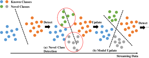
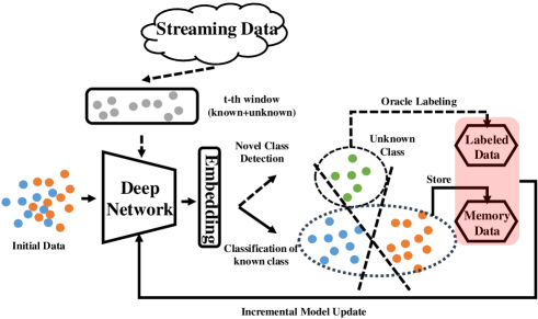
Traditional closed set recognition (CSR) assumes that training and testing data are draw from the same space, i.e., the label and feature spaces, and various methods have achieved significant success in different applications [1, 2]. However, the real-world is dynamically changing, and many applications are non-stationary, which always receive the data as streaming form and many unknown classes will emerge sequentially, for example, driverless cars need to identify unknown objects, face recognition needs to distinguish unseen personal pictures, image retrieval often appears with new categories, etc. This is defined as class-incremental learning (CIL) in literature, which is more challenging and practical than CSR. As shown in Figure 1, CIL includes two key components: novel class detection (NCD) and incremental model update (IMU). The main difficulty of NCD is to effectively distinguish the known and unknown classes, i.e., the instances from novel classes during testing, which are unknown in training phase as shown in Figure 1 (a). Meanwhile, after novel class detection, we also need to consider the IMU, which aims to re-train the model with newly labeled instances from unknown classes as shown in Figure 1 (b). Consequently, streaming test data continue to present novel classes, and we need to conduct the NCD and IMU operators iteratively.
To address the NCD issue, zero-shot learning (ZSL) is firstly proposed [3, 4], which aims to classify instances from unknown categories, by merely utilizing seen class examples and semantic information about unknown classes. Whereas the standard ZSL methods only test unknown classes, rather than test both known and unknown classes. Thus, generalized zero-shot learning (GZSL) is proposed, which automatically detect known and unknown classes simultaneously. For example, Lampert et al. introduced an attribute-based classification method, which detected new objects based on a high-level description in terms of semantic attributes [6]; Changpinyo et al. proposed a GZSL method via manifold learning, which was to align the semantic space with visual features [7]; Li et al. introduced the feature confusion GAN, which proposed a boundary loss to maximize the decision boundary of seen categories and unseen ones [8]. However, both ZSL and GZSL assume that semantic information (for example, attributes or descriptions) of the unknown classes is given, which is limited to detect with prior knowledge, and have no ability to detect incrementally.
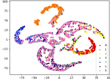
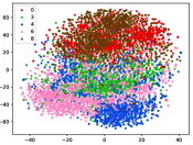
Therefore, a more realistic prediction is to detect unknown classes without any information, either instances or side-information during training. Recent NCD approaches usually leverage the powerful deep neural networks, and can mainly be divided into two aspects: discriminative and generative models. Discriminative models mainly utilize the powerful feature learning and prediction capabilities of deep models to design corresponding distance or prediction confidence measures. For example, Bendale and Boult proposed the OpenMax model, which trained a deep neural network with the normal SoftMax layer by using the Weibull distribution fitting score [9], yet it failed to recognize the adversarial images which are visually indistinguishable from training instances; Hassen and Chan learned the neural network based representation, which restricted the inter-class and intra-class distances during training, thus to lead larger spaces for novelty detection [10]. However, as shown in Figure 2 (a) and (b), it is notable that on simple visual datasets such as MNIST, known and unknown classes have strong separability on the trained model, thereby the distance measure is more effective. Whereas in more complex visual datasets such as CIFAR-10, unknown and known categories have embedding confusion in feature space, i.e, instances of unknown and known classes are mixed, thus the performance of distance measure based methods will greatly reduce. On the other hand, Generative models mainly employ the adversarial learning to generate instances that can fool the discriminative model, thus to detect the novel class. Ge et al. utilized the generative model to generate unknown class instances near the decision margin, which can provide explicit probability estimation over generated unknown class [11]. However, as shown in Figure 2 (c) and (d), we can get similar conclusions to discriminative model, i.e., generated instances on complex datasets such as CIFAR-10 are almost uselesss, which is also mentioned in [13]. Besides, most existing detection methods are limited to detect single novel class, i.e., they assume that only one novel class appears at each period.
Furthermore, we need incremental model update (IMU) with the newly labeled instances of novel classes after detecting. Different from re-training with all previous known data, IMU aims to re-train the model only referring no or limited known data, which can ensure the efficiency of incremental update. Therefore, a big challenge for IMU is the catastrophic forgetting phenomenon [14], i.e., we can find that the knowledge learned from the previous task (known classes classification) will be lost when information relevant to the current task (novel class classification) is incorporated. To mitigate the catastrophic forgetting, there are many attempts, including replay-based methods that explicitly re-train on stored examples while training on new tasks [15, 16], and regularization-based methods that utilize extra regularization term on output or parameters to consolidate previous knowledge [13, 17, 18].
(a) DM on MNIST
(b) DM on CIFAR-10
(c) GM on MNIST
(d) GM on CIFAR-10
To this end, we propose a Class-Incremental Learning without Forgetting (CILF) framework, which aims to process new class detection and model update iteratively. In detail, we firstly develop a novel decoupled prototype based network to train the known classes, which employs the constrained clustering loss to regularize the inter-class and intra-class structure. In testing, considering emergence of single or multiple novel classes, we develop the curriculum operator for learning adaptive embedding, which aims to conduct learnable clustering from easy to hard instances and overcome the embedding confusion. Then, with the limited memory data of known classes, CILF updates the network with robust regularization to mitigate the catastrophic forgetting. In summary, the main contributions are summarized as follows:
-
•
Propose the “ Class-Incremental Learning without Forgetting” (CILF) framework, which considers both novel class detection and incremental model update;
-
•
Propose a novel decoupled prototype based network, which can conduct novel class detection and model update effectively;
-
•
Propose curriculum clustering operator for better multiple novel classes detection and robust regularization to mitigate catastrophic forgetting.
In remaining sections of this paper, section 2 introduces the related work. Section 3 presents the proposed method. Section 4 evaluates the proposed method. Finally, the whole work is concluded in Section 5.
2 Related Work
Our work aims to detect novel classes in streaming data, and update the model with limited known data without forgetting. Therefore, our work is related to: novel class detection and incremental model update.
Traditional novel class detection approaches mainly restrict intra-class and inter-class distance property in training data, then detect novel class by identifying outliers. For example, Da et al. developed a SVM-based method, which learned the concept of known classes while incorporating the structure presented in the unlabeled data collected from open set [19]; Mu et al. proposed to dynamically maintain two low-dimensional matrix sketches for detecting novel classes [20]. However, these approaches are difficult to process high dimensional space considering complex matrix operations. Recently, with the development of deep learning techniques, several studies have applied convolutional neural network (CNN) on the detection scenario. Hendrycks and Gimpel verified that CNN trained on the MNIST images can predict high confidence (90) on gaussian noise instances, thus we can use the softmax output probabilities to distinguish known/unknown class [21]. Furthermore, Liang et al. directly utilized temperature scaling or added small perturbations to separate the softmax score distributions between in- and out-of-distribution images [22]; Neal et al. introduced a novel augmentation technique, which adopted an encoder-decoder GAN architecture to generate the synthetic instances similar to known class [13]; Wang et al. proposed a cnn-based prototype ensemble method, which adaptively update the prototype for robust detection [17]. Nevertheless, these methods always limited to detect single novel class in once time. Therefore, Han et al. proposed an extended deep transfer embedded clustering method for multiple novel class detection [24]. Nevertheless, existing NCD methods usually have superior detection performance on simple datasets, but are easily interfered by embedding confusion on complex datasets.
Incremental learning is always applied for streaming data. In most situations, only a few examples from known classes/features/distributions are available in the beginning and data with new classes/features/distributions emerge thereafter. Incremental learning methods aim to update the models from streaming data sequentially only with newly coming data and limited previous data, without re-training with all previous data [25]. As a matter of fact, incremental deep learning can directly apply with online backpropagation, yet with one important drawback: catastrophic forgetting, which is the tendency for losing the learned knowledge of previous distribution (previously known classes/features/distributions). To solve this problem, there are many attempts, for example, Rebuffi et al. stored a subset of examples per class, which are selected to best approximate the mean of each class in the feature space [15], Lopez-Paz and Ranzato projected the estimated gradient direction on the feasible region outlined by previous tasks through a first order Taylor series approximation [26]; Li and Hoiem utilized the output of previous model as soft labels for previous tasks [27]; Kirkpatrick et al. proposed the elastic weight consolidation to reduce catastrophic forgetting [28]; Lee et al. proposed to incrementally match the moment of posterior distribution of the neural network [29].
3 Proposed Method
In this section, we formalize the problem of class-incremental learning with streaming data, and give the details of proposed framework.
3.1 Problem Definition
Without any loss of generality, at initial time, we have a supervised training set , where denotes the th instance, and denotes corresponding label, represents initial time. Then, we receive a non-stationary unlabeled testing data , where denotes the th instance, and label is unknown, is the number of unknown classes. Thus, novel class detection can be defined as:
Definition 1
Novel Class Detection (NCD) With the initial training set , we aim to construct a model, i.e., . Then with the pre-trained model , novel class detection is to classify the known and unknown classes in accurately.
On the other hand, it is notable that streaming data with novel classes has two characteristics: (1) Data window. At time window , we only get the data of current time window, not the full amount of streaming data for detection; and (2) Novel class continuity. At time window , only partial novel classes will appear, or even no novel classes. Therefore, we need to incrementally detect novel classes, i.e., with the streaming data, every time after receiving the data of time window , NCD is performed [30]. Specifically, the streaming test data can be denoted as , where is with unlabeled instances, and the underlying label is unknown, , where is the cumulative known classes until th time window and is the new classes in th window. . Therefore, we can give the definition of class-incremental learning:
Definition 2
Class-Incremental Learning (CIL) At time , we have pre-trained model and finite stored instance set from known classes until th time, and receive streaming data . First, we aim to classify known and unknown classes in as Definition 1. Then, with the newly labeled data from novel classes and stored data , we update the model while mitigating forgetting to acquire . Cycle this process until terminated.
Note that there exist two labeling cases after novel class detection, i.e., manually labeling or self-taught labeling [20]. We consider manually labeling following most approaches [30, 20, 17] to avoid label noise accumulation, and is more in line with real-world applications.
3.2 CILF Framework
The main idea of CILF is to learn the feature embeddings such that instances exhibit distinguishing characteristics for label prediction, novel class detection, and subsequent model update over the non-stationary streaming data. Therefore, the most critical parts of CILF are: (1) feature embedding network; (2) novel class detection operator; and (3) model update mechanism.
-
•
Feature Embedding Network: With the initial training data, i.e., the blue and orange dots as shown in figure 3, the decoupled neural network model is trained using the labeled initial data with the prototype based loss, which concerns the intr-class/inter-class structure and can be easily transformed for NCD;
-
•
Novel Class Detection Operator: At time , we receive a set of unlabeled data from the streaming data, i.e., gray dots as shown in figure 3, which includes known (blue and orange dots) and unknown (green dots) classes. The observed instances set are transformed through learned network, and achieve feature representations. Then we employ the pre-trained for curriculum clustering operating, which can detect multiple unknown classes from easy to difficult in self-taught form;
-
•
Model Update Mechanism: After NCD, true labels of instances from novel classes are queried (partially or fully), then IMU is performed on with the newly labeled data, while regularizing the performance of stored data from known classes to mitigate forgetting. The updated model is then used to further classify incoming instances along the stream.
This process is repeated until the end of streaming data. Figure 3 illustrates the overall streaming data classification performed by CILF framework. And Table I provides the definition of symbols used in this paper.
| Sym. | Definition |
|---|---|
| initial supervised training data | |
| set of unlabeled data at th time window | |
| set of labeled new class data at time | |
| label set at th time window | |
| trained model th time window | |
| stored memory data of known classes | |
| until th time window | |
| feature embedding of instance | |
| prediction of th instance at time | |
| prototype of th class at time | |
| weight of each instance at time | |
| pacing function to determine the number of | |
| selected instances in each mini-batch |
3.3 Feature Embedding Network
Given the initial training data , our primary objective is to build an effective model for subsequent classification. Recent researches have demonstrated the effectiveness of deep model on feature embedding and subsequent tasks, thereby we employ the deep models for building , for example, convolution neural networks for images. Importantly, the built deep model needs to consider two aspects: (1) Distance measure. The model needs to emphasize the exploitation of feature embeddings considering intra-class compactness and inter-class separability, thus leave larger space for novel class detection; (2) Model scalability. The model needs to effectively learn novel class knowledge and incrementally update model with the emergence of novel class data. However, traditional deep models using cross entropy cannot consider the distance measure effectively, and are difficult to conduct the model update (the prediction layer is coupled to the fully connected layer, and is difficult to expand). Consequently, we develop a decoupled deep embedding network with prototype based loss to improve the inter-class and intra-class structure.
Particularly, for a given input , the output feature representations are denoted as , is the correspond network parameters, and we utilize notation for clarity. Inspired from the topic of metric learning [31], the loss can be defined as:
| (1) |
where aims to pull data towards their neighbor from same class, and is to push data away from different classes. is the balance parameter.
3.3.1 Intra-Class Compactness
can be obtained by calculating the distance between each instance and corresponding prototype, here we utilize the class center. Similar to cross entropy loss [32], i.e., , where is the ground truth of th instance, denotes the fully connected layer with softmax function. is depending on the feature output . Consequently, we define the prototype-based cross entropy loss as following:
| (2) |
where is the probability of being classified as , which is negatively related to the distance between instance and prototype of th class, i.e., the probability is larger if the distance is closer, otherwise is smaller. Thus the , where is the representations of th class prototype, and can be defined as following:
| (3) |
where is the class number, and is a hyperparameter that controls the strength of distance similar to large margin cross-entropy [33]. Note that Eq. 3 minimizes loss via maximizing the probability of being associated with the prototype . Moreover, it is crucial to initialize and update each class prototype effectively. The labels of initial training data are given, thereby we use the output representation , for each prototype initialization:
where is the size of th class. On the other hand, the key idea of prototype update is to anneal clusters slowly to eliminate the biased instances in each mini-batch. Thus we propose to smooth the annealing process via temporal ensemble [34]:
| (4) |
where is a momentum term controlling the ensemble, and indicates the th epoch for the initial training.
3.3.2 Inter-Class Separability
The prototype-based cross entropy loss guarantees the local intra-class compactness, while neglects the inter-class separability. To make the projection of instances robust in distance measure, focuses on improving global separation between different classes. Particularly, aims to transform instances from similar classes to be closer than those from different classes, i.e., , where share same class and is from different class, is a metric function measuring distances in the embedding space, and we use notation for clarity. This is known as the triplet loss with a pre-specified margin value , i.e., . It is notable that triplet loss always suffers from slow convergence, thus triplet construction is central for improving the performance. Inspired by [35], we consider the hard triplet to fully explore multiple negative examples from different classes in each mini-batch, which can further improve the inter-class distances. In result, hard triplet is denoted as:
| (5) |
where is the class number and negative examples is from different classes. Eq. 5 can better consider the global inter-class distances. Thereby the can be defined as:
| (6) |
where denotes the hard triplet set. Here we utilize euclidean distance to evaluate the distance between two examples:
| (7) |
Consequently, we can learn discriminative feature embedding, and boost the performance of classification and detection via optimizing Eq. 1: (1) Prototype-based loss highlights the compactness of representation, i.e., the intra-class would be more compact and inter-class would be more distant. This property is suited for distinguishing the known and unknown classes; and (2) Prototype-based loss is based on the feature output embedding, which is independent of prediction layer. Therefore, it is easy to update the model and learn novel classes, without the expansion of model structure (prediction layer). The details are shown in Algorithm 1.
-
•
Input:
-
•
Data set:
-
•
Parameter: , , Learning rate parameter:
-
•
Output:
-
•
Decoupled deep clustering network:
3.4 Novel Class Detection
Traditional closed-set methods predict the known classes of training phase, in which the number of possible labels at testing is known and fixed. However, in class-incremental setting, instances belonging to unknown classes may appear with the streaming test data. Therefore, we need to distinguish the known and unknown classes. Specifically, we receive a set of unlabeled data at th time, and there may occur novel classes, where . However, most current detection methods either assume that only one novel class appears per time, i.e., , or classify multiple novel classes as a super-class, which is impractical and difficult to operate considering efficiency. To solve this problem, we aim to fine-tune the deep clustering network of last time for multiple novel class detection. As shown in Figure 2, a key challenge is that adversarial instances of novel classes are mixing with known classes in complex scenario, leading the embedding confusion and greatly affecting the clustering effect, i.e., biased prototypes for known and unknown classes. To solve this problem, we employ a learnable curriculum clustering operator, which aims to conduct clustering from easy (distinguishable) to difficult (confused) instance via curriculum learning [36]. Consequently, we can acquire more reliable prototype and novel class detection result.
In detail, considering the model training in Algorithm 1 is entirely supervised, whereas is unsupervised, we aim to discover novel classes in by unsupervised clustering, which fine-tunes the trained on phase with easy instances first, and then cluster the mixed ones. We address this challenge by decomposing the learnable curriculum clustering into two closely related sub-tasks as curriculum learning. The first is weighting function to calculate the weight of each instances, and initialize the prototype with weighted k-means. The second is pacing function to determine the pace for which data are presented to fine-tune the model, thus conduct curriculum clustering.
3.4.1 Weighting Function
Inspired by [37], we evaluate the weight of each instance by self-taught weighting function. In detail, we compute confidence score for each instance in using existing model . We first obtain the statistic confidence by applying intra-class distance using Eq. 2, i.e., . It is notable that of the instance near prototype are smaller, and of the instances away from all class prototypes are larger. Therefore, the weight of each instance can be denoted as , where is the threshold parameter. Thereby the highly confident and unsure instances have larger weights, and confusing ones have lower weights.
On the other hand, Algorithm 1 requires initial setting for prototypes . Thus we initialize prototypes by running semi-supervised weighted k-means algorithm [38] by combing the unlabeled set and pre-trained . In result, we can obtain more robust initial prototypes:
| (8) |
where is the set of the class, in which the pseudo-label of each instance can be calculated by Eq. 3.
3.4.2 Pacing Function
A direct way for classifying known and unknown classes in is to fine-tune using all the instances. However, considering the embedding confusion, the initialized prototypes are biased and pseudo-labels exist noises. If we randomly sample batches from the full amount of data to fine-tune model, the embedding confusion will further affect the update of prototypes and pseudo-labels. Therefore, we turn to sort the instances according to difficulty, and present from easier to harder instances for fine-tuning with the model capability increase, rather than giving a sequence of mini-batches uniformly from in most common training procedure, is the number of batches.
In detail, the pacing function is used to determine a sequence of subsets , of size . The -th subset includes the first elements of the instances, which are sorted by the scoring function in ascending order. Here, we utilize the fixed exponential pacing, which has a fixed step length, and exponentially increasing size in each batch. Formally, it is given by:
| (9) |
Where denotes the fraction of data in the initial step, is the exponential factor for increasing the size of sampled mini-batches in each step, is the number of iterations in each step, denotes round down, is the index of batches, is the number of instances. Consequently, in each mini-batches, we select episodic data with variable length for reliable fine-tuning.
3.4.3 Fine-tune Clustering
With the sampled mini-batches in each epoch, we aim to fine-tune the from easier to harder, and Eq. 2 can be reformulated as:
| (10) |
where denotes the triplet set of th batch. aims to constraint the updated prototypes of known classes approaching the pre-trained ones, which can regularize the embeddings of known classes. The pseudo-labels for each instance can be calculated by Eq. 3. So far, we assume that the number of classes is known, which is impractical in real applications. Thus we aim to estimate the number of classes in the unlabeled data. Specifically, we fine-tune clustering using by varying the number of unknown classes. The resulting clusters are then examined by computing cluster validity index (CVI), which concerns the intra-cluster cohesion vs inter-cluster separation. And we select the generally used Silhouette index [39]:
| (11) |
where is the average distance between and all other data instances within the same cluster, and is the smallest average distance of to all instances in any other different cluster. The optimal number of categories is the inflection point of CVI with maximum curvature. The details are shown in Algorithm 2.
-
•
Input:
-
•
Data set:
-
•
Parameter: , , , ,
-
•
Output:
-
•
Novel Class Detection Network:
3.5 Incremental Model Update
Ideally, the initial model training and novel class detection processes can identify the known and unknown classes. However, considering streaming data with unceasing novel class, we need reliable training data of novel classes to create new prototypes and update the model parameters in incremental fashion. Thus, we need to collect novel class data for labeling, which can be used to re-train . Similar to previous studies [40, 20], after curriculum clustering operator for detection, we can achieve potential novel class instances for querying their true labels. Note that we can query full or only partial data of novel class. However, there exist catastrophic forgetting of known classes if we only use the new data to update the model.
To solve this problem, we develop a mechanism to incorporate the stored memory and novel class information incrementally, which can mitigate the forgetting of discriminatory characteristics about known classes. In detail, we utilize the exemplary data for regularization in re-training:
| (12) |
The first term encourages the network to output the correct class indicator (classification loss) for all labeled examples, i.e., and , and reproduces the scores calculated in the previous step (distillation loss) for stored in-class examples, i.e., . is constituted from and . After re-training, we need to update the to store key points of novel classes, we randomly remove instances for each known class, and sample instances for each novel class. The details are shown in Algorithm 3.
-
•
Input:
-
•
Data set: memory data , labeled novel class data
-
•
Learning rate parameter:
-
•
Output:
-
•
Re-trained deep clustering Network:
4 Experiments
In this section, we mainly verify the proposed CILF from two aspects: (1) classification of known and novel classes; and (2) forgetting of known classes. Considering that most large-scale datasets are concentrated on images, thus we empirically evaluate CILF comparing with the state-of-the-art approaches on four simulated stream image datasets.
(a) Single Novel Class
(b) Multiple Novel Classes
| Methods | Average NA | Average Macro-F-Measure | ||||||
|---|---|---|---|---|---|---|---|---|
| MNIST | CIFAR-10 | CIFAR-50 | CIFAR-100 | MNIST | CIFAR-10 | CIFAR-50 | CIFAR-100 | |
| Iforest | .189.021 | .131.023 | .045.006 | .040.004 | .156.023 | .096.011 | .035.005 | .027.004 |
| One-SVM | .211.032 | .136.031 | .043.007 | .039.000 | .135.021 | .090.014 | .032.003 | .024.005 |
| LACU-SVM | .222.034 | .141.020 | .045.005 | .039.004 | .170.018 | .096.010 | .034.004 | .026.006 |
| SENC-MAS | .203.030 | .134.033 | .043.006 | .038.001 | .149.031 | .082.013 | .031.003 | .022.005 |
| ODIN-CNN | .293.011 | .194.020 | .068.001 | .034.027 | .323.029 | .156.033 | .031.002 | .055.045 |
| CFO | .276.008 | .202.015 | .037.001 | .022.008 | .292.022 | .167.025 | .045.002 | .033.013 |
| CPE | .298.013 | .250.020 | .055.001 | .047.017 | .337.034 | .281.033 | .109.002 | .087.031 |
| DEC | .289.058 | .245.152 | .035.001 | .027.001 | .357.081 | .261.344 | .048.001 | .018.001 |
| CILF | .371.022 | .288.034 | .092.008 | .055.004 | .365.012 | .302.033 | .158.005 | .092.008 |
| Methods | Average Micro-F-Measure | Average AUROC | ||||||
|---|---|---|---|---|---|---|---|---|
| MNIST | CIFAR-10 | CIFAR-50 | CIFAR-100 | MNIST | CIFAR-10 | CIFAR-50 | CIFAR-100 | |
| Iforest | .234.036 | .142.021 | .066.008 | .052.008 | .083.014 | .140.343 | .077.014 | .105.009 |
| One-SVM | .214.074 | .147.031 | .064.008 | .046.007 | .117.009 | .101.021 | .096.011 | .074.020 |
| LACU-SVM | .258.042 | .148.022 | .064.007 | .050.008 | .123.013 | .068.012 | .089.016 | .117.081 |
| SENC-MAS | .216.065 | .140.036 | .062.008 | .044.006 | .104.036 | .082.026 | .043.010 | .079.096 |
| ODIN-CNN | .285.021 | .188.040 | .035.001 | .058.041 | .259.189 | .185.063 | .102.045 | .123.096 |
| CFO | .351.016 | .304.030 | .054.001 | .047.017 | .208.180 | .162.073 | .076.030 | .102.092 |
| CPE | .336.026 | .299.040 | .110.001 | .092.033 | .270.184 | .193.060 | .114.037 | .119.100 |
| DEC | .323.073 | .289.305 | .064.001 | .025.001 | .264.187 | .190.058 | .108.036 | .114.097 |
| CILF | .355.025 | .310.025 | .122.008 | .103.008 | .317.018 | .255.039 | .125.012 | .130.027 |
(a-1) Original-1
(a-2) Original-2
(a-3) Original-3
(a-4) Original-4
(a-5) Original-5
(a-6) Original-6
(b-1) CPE-1
(b-2) CPE-2
(b-3) CPE-3
(b-4) CPE-4
(b-5) CPE-5
(b-6) CPE-6
(c-1) DEC-1
(c-2) DEC-2
(c-3) DEC-3
(c-4) DEC-4
(c-5) DEC-5
(c-6) DEC-6
(d-1) CILF-1
(d-2) CILF-2
(d-3) CILF-3
(d-4) CILF-4
(d-5) CILF-5
(d-6) CILF-6
| Methods | Forgetting | |||
|---|---|---|---|---|
| MNIST | CIFAR-10 | CIFAR-50 | CIFAR-100 | |
| Iforest | .027.006 | .021.002 | .043.001 | .067.001 |
| One-SVM | .028.007 | .019.004 | .042.002 | .068.002 |
| LACU-SVM | .032.005 | .029.002 | .038.003 | .061.001 |
| SENC-MAS | .028.005 | .020.001 | .036.002 | .060.001 |
| ODIN-CNN | .040.004 | .012.006 | .023.002 | .018.005 |
| CFO | .023.012 | .010.003 | .014.001 | .016.005 |
| CPE | .022.001 | .007.001 | .017.001 | .013.003 |
| DEC | .026.005 | .009.001 | .015.002 | .014.001 |
| DNN-Base | .042.005 | .012.007 | .015.003 | .024.006 |
| DNN-L2 | .032.010 | .011.004 | .012.007 | .029.003 |
| DNN-EWC | .023.014 | .016.010 | .014.009 | .016.007 |
| IMM | .030.012 | .009.003 | .016.004 | .025.004 |
| DEN | .024.003 | .007.004 | .011.009 | .017.001 |
| CILF | .020.016 | .006.001 | .010.001 | .013.003 |
(a) NA
(b) Macro-F-Measure
(c) Micro-F-Measure
(d) AUROC
4.1 Datasets
We utilize three commonly used visual datasets for class-incremental scenario following [17, 30, 13], including MNIST [41], CIFAR-10 [42], CIFAR-100 111http://www.cs.toronto.edu/kriz/cifar.html. In detail, MNIST dataset contains labeled handwritten digits images from 10 categories, where each class contains between 6313 and 7877 monochrome images; CIFAR-10 dataset has a total of 60000 color images of 32x32 pixels from 10 natural image classes; CIFAR-100 dataset is enlarged CIFAR-10, and we structure CIFAR-100 into 2 datasets: CIFAR-50 and CIFAR-100 according to [13].
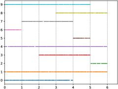
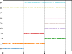
Inspired from [43, 17, 30, 13, 44], we utilize the given testing data from the raw datasets as a holdout set to evaluate forgetting, and use the given training data to generate the streaming data. Specifically, we rearrange instances in each dataset to emulate a streaming form with novel classes considering two forms: (1) single novel class each time window; (2) multiple novel classes each time window. For single novel class case, we randomly choose initial classes, and only 1 novel class may start for each time window. In order to be more in line with real-world applications, each known class may disappear randomly at the end of current time window. Specifically, we set for MNIST and CIFAR-10, for CIFAR-50, for CIFAR-100. Figure 4 (a) presents a simulated example of the CIFAR-10, i.e., we randomly choose 5 initial classes, and there are 5 time windows with 1 novel class starting for each time window. For multiple novel class case, we randomly choose initial classes, and novel classes (i.e., novel classes) may randomly start for each time window. Similar to single class setting, each class may disappear randomly. Specifically, we set for MNIST and CIFAR-10, for CIFAR-50, for CIFAR-100. Figure 4 (b) presents a simulated example of the CIFAR-10, i.e., we choose 3 initial classes and there are 3 time windows, 2 novel classes start for the first time window, 3 novel classes for the second time window, 2 novel classes for the last window.
| Methods | Average NA | Average Macro-F-Measure | ||||||
|---|---|---|---|---|---|---|---|---|
| MNIST | CIFAR-10 | CIFAR-50 | CIFAR-100 | MNIST | CIFAR-10 | CIFAR-50 | CIFAR-100 | |
| Iforest | .348.069 | .277.062 | .133.021 | .095.014 | .181.062 | .103.004 | .040.004 | .028.002 |
| One-SVM | .361.085 | .277.049 | .136.017 | .089.014 | .188.085 | .107.008 | .038.005 | .026.003 |
| LACU-SVM | .357.054 | .274.062 | .133.012 | .090.017 | .191.054 | .098.008 | .032.005 | .023.002 |
| SENC-MAS | .336.075 | .280.050 | .139.021 | .091.013 | .163.071 | .106.002 | .035.004 | .024.002 |
| ODIN-CNN | .396.021 | .304.039 | .181.008 | .071.007 | .268.032 | .243.005 | .160.006 | .054.004 |
| CFO | .353.012 | .287.027 | .212.009 | .104.008 | .380.021 | .363.001 | .288.007 | .183.005 |
| CPE | .413.030 | .401.061 | .240.020 | .132.020 | .236.047 | .339.037 | .249.022 | .244.021 |
| DEC | .350.142 | .398.084 | .206.012 | .089.016 | .327.315 | .302.217 | .230.017 | .110.011 |
| CILF | .493.051 | .422.054 | .258.040 | .179.031 | .392.045 | .407.033 | .332.035 | .259.041 |
| Methods | Average Micro-F-Measure | Average AUROC | ||||||
|---|---|---|---|---|---|---|---|---|
| MNIST | CIFAR-10 | CIFAR-50 | CIFAR-100 | MNIST | CIFAR-10 | CIFAR-50 | CIFAR-100 | |
| Iforest | .272.079 | .153.009 | .067.002 | .049.003 | .140.015 | .126.019 | .113.023 | .140.009 |
| One-SVM | .293.122 | .161.018 | .068.008 | .045.003 | .158.016 | .153.011 | .146.008 | .092.010 |
| LACU-SVM | .294.060 | .144.006 | .062.006 | .043.002 | .149.002 | .158.016 | .145.005 | .152.024 |
| SENC-MAS | .250.082 | .165.012 | .063.008 | .045.004 | .107.092 | .123.006 | .086.051 | .043.032 |
| ODIN-CNN | .242.024 | .193.006 | .072.009 | .067.006 | .231.052 | .145.245 | .193.140 | .133.250 |
| CFO | .245.016 | .212.004 | .108.010 | .104.008 | .195.050 | .214.257 | .115.145 | .159.245 |
| CPE | .207.037 | .367.035 | .200.023 | .146.022 | .241.056 | .255.243 | .201.140 | .183.254 |
| DEC | .294.292 | .231.204 | .141.016 | .116.011 | .234.061 | .217.076 | .197.137 | .171.253 |
| CILF | .422.043 | .442.043 | .212.022 | .152.016 | .286.028 | .261.022 | .189.034 | .192.016 |
| Methods | Forgetting | |||
|---|---|---|---|---|
| MNIST | CIFAR-10 | CIFAR-50 | CIFAR-100 | |
| Iforest | .014.015 | .006.004 | .035.002 | .048.005 |
| One-SVM | .018.010 | .005.003 | .033.004 | .049.003 |
| LACU-SVM | .017.010 | .004.002 | .029.003 | .042.004 |
| SENC-MAS | .011.011 | .006.002 | .032.002 | .041.004 |
| ODIN-CNN | .011.008 | .013.011 | .015.006 | .013.010 |
| CFO | .019.005 | .008.006 | .009.008 | .023.003 |
| CPE | .007.001 | .011.003 | .009.002 | .005.002 |
| DEC | .002.003 | .009.001 | .006.002 | .023.001 |
| DNN-Base | .022.002 | .023.009 | .032.007 | .039.006 |
| DNN-L2 | .021.002 | .026.001 | .035.005 | .041.002 |
| DNN-EWC | .016.010 | .017.010 | .020.005 | .021.009 |
| IMM | .022.030 | .023.010 | .024.012 | .030.019 |
| DEN | .010.009 | .013.005 | .013.002 | .021.011 |
| CILF | .001.001 | .005.001 | .001.001 | .008.001 |
4.2 Compared Methods
To validate the effectiveness of proposed CILF, we compared with existing state-of-the-art novel class detection approaches and incremental learning methods.
First, we compared CILF with existing NCD and incremental NCD methods. Including traditional anomaly detection and linear methods: Iforest [45], One-Class SVM (One-SVM) [ScholkopfPSSW01], LACU-SVM (LACU) [19], SENC-MAS (SENC) [20]; deep methods: ODIN-CNN (ODIN) [22], CFO [13], CPE [17] and DTC [24]. Abbreviations in parentheses. DTC is clustering based methods for multiple unknown classes detection. Note that Iforest, One-SVM, LACU, ODIN, CFO, and DTC are NCD methods, SENC and CPE are incremental NCD methods. All NCD baselines except Iforest can be updated incrementally using newly labeled unknown class data and memory data.
-
•
Iforest: an ensemble tree method to detect outliers;
-
•
One-Class SVM (One-SVM): a baseline for out-of-class detection and classification;
-
•
LACU-SVM (LACU): a SVM-based method that incorporates the unlabeled data from open set for unknown class detection;
-
•
SENC-MAS (SENC): a matrix sketching method that approximates original information with a dynamic low-dimensional structure;
-
•
ODIN-CNN (ODIN): a CNN-based method that distinguishes in-distribution and out-of-distribution over softmax score;
-
•
CFO: a generative method that adopts an encoder-decoder GAN to generate synthetic unknown instances;
-
•
CPE: a CNN-based ensemble method, which adaptively updates the prototype for detection;
-
•
DTC: an extended deep transfer clustering method for novel class detection.
Specifically, 1) Iforest, ODIN and CFO can only perform binary classifications, i.e., whether the instance is an unknown class. Thus we further conduct unsupervised clustering on both know and unknown class data for subdividing; 2) all baselines are one-class methods except DTC, i.e., they perform NCD in two steps: first detect the super-class of unknown classes, then perform unsupervised clustering; 3) all of baselines are NCD methods except LACU, SENC and CPE, but they can be applied in incremental NCD by combing memory data to update following [17].
To validate the incremental model update, we also compare with state-of-the-art forgetting methods: DNN-Base, DNN-L2, DNN-EWC [28], IMM [29], DEN [46], each time window is regarded as a task in these methods. In detail, the compared methods are:
-
•
DNN-Base: Base DNN with -regularizations;
-
•
DNN-L2: Base DNN, where at each stage t, is initialized as and continuously trained with -regularization between and ;
-
•
DNN-EWC: Deep network trained with elastic weight consolidation for regularization, which remembers old stages by selectively slowing down learning on the weights important for those stages;
-
•
IMM: An incremental moment matching method with two extensions: Mean-IMM and Mode-IMM, which incrementally matches the posterior distribution of the neural network trained on the previous stages;
-
•
DEN: A deep network architecture for incremental learning, which can dynamically decide its network structure with a sequence of stages and learn the overlapping knowledge sharing structure among stages.
4.3 Evaluation Metrics
Considering that CILF can distinguish the known and unknown classes, while mitigating the forgetting. Thus we measure the proposed method from two aspects: (1) NCD performance; (2) Forgetting performance.
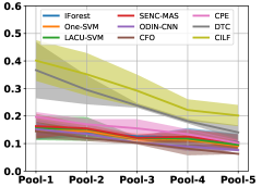
Following [30], we adopt the commonly used evaluation metrics for novel class detection: 1) Normalized Accuracy (NA), which weights the accuracy for known and novel classes [47]; 2) Macro-F-measure and Micro-F-measure; and 3) AUROC, which considers the NCD task as a combination of novelty detection and multi-class recognition [13]. Moreover, to validate the catastrophic forgetting, we calculate the performance about forgetting profile of different learning algorithms as [44], i.e., let be the accuracy evaluated on the hold-out sets, i.e. the novel classes emerge on th time window (), after training the network incrementally from stage 1 to , the average accuracy at time is defined as: [44]. higher represents for better classifier. , is the optimal accuracy with the entire data. We repeat all experiments with 5 times, and record the mean and std.
(a-1) Original-1
(a-2) Original-2
(a-3) Original P3
(a-4) Original-4
(a-5) Original-5
(b-1) CPE-1
(b-2) CPE-2
(b-3) CPE-3
(b-4) CPE-4
(b-5) CPE-v5
(c-1) DEC-1
(c-2) DEC-2
(c-3) DEC-v3
(c-4) DEC-4
(c-5) DEC-5
(d-1) CILF-1
(d-2) CILF-2
(d-3) CILF-3
(d-4) CILF-4
(d-5) CILF-5
(a) NA
(b) Macro-F-Measure
(c) Micro-F-Measure
(d) AUROC
4.4 Implementation
We develop CILF based on convolutional network structure as ResNet18 [48]. Note that we use an identical set of hyperparameters (, , , , , , ). In all of our models and experiments, we adopt standard SGD with Nesterov momentum [49], where the momentum is 0.9. We train the initial model as following: the number of epochs is 20, the batch size is 128, the learning rate is 0.01, and weight decay is 0.001. We implement all baselines and perform all experiments based on code released by corresponding authors. For CNN based methods, we use the same network architecture and parameters during training, such as optimizer, learning rate schedule, and data pre-processing. Our method is implemented on a RTX 2080TI GPU with Pytorch 0.4.06 222https://pytorch.org/.
4.5 Single Novel Class Detection
Table II compares the detection performance of CILF with all baseline methods on each streaming data with single novel class. We observe that: (1) CNN-based methods are better than traditional detection approaches, i.e., One-SVM, LACU-SVM, SENC-MAS. This indicates that neural network provides superior feature embeddings for prediction and detection over high dimensional streaming data; (2) CILF consistently outperforms all compared CNN-based methods in all the criteria. For example, in CIFAR-10, CILF provides at least 2 improvements than other methods. This indicates the effectiveness of prototype based loss for feature embedding and curriculum clustering operator for detection; and (3) The detection performance for large-scale data sets still needs to be improved, and the results of all methods are low.
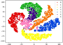
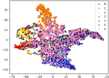
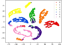
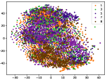
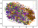
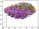
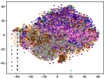
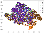
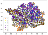
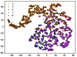
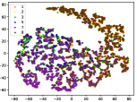
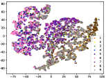
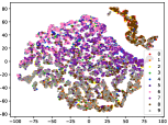
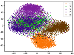
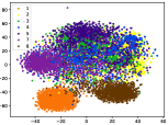
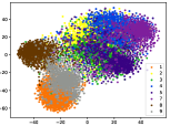
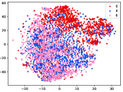
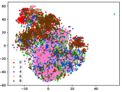
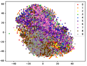
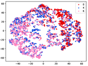
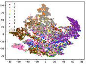
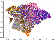
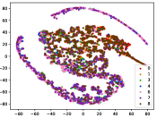
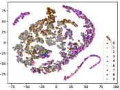
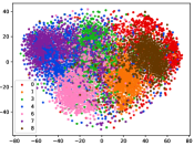
Figure 5 shows feature embedding results within each time window using T-SNE [50], in which each class randomly samples 800 instances. Note that we turn to utilize the more complex dataset CIFAR-10 as an example, rather than simpler MNIST dataset in previous methods. Clearly, the optimal discriminative method (CPE) and generative method (DEC) are greatly interfered by the embedding confusion. While the output of CILF has more distinct groups from different classes compared to other methods, which is attributed to the prototype based loss for model training. Moreover, instances from novel classes are well separated from other known clusters, which is benefit for novel class detection. The compactness of new class indicates the effectiveness of curriculum clustering operator, in which reliable prototypes are developed and the the model is fine-tuned from easy to difficult.
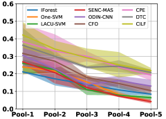
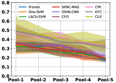
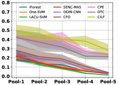
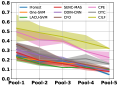
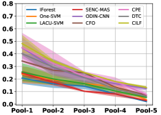
Table III compared the forgetting performance of CILF with all baseline methods, which defines the forgetting of emerge class on a particular window, i.e., the difference between maximum knowledge gained about that window throughout learning process and we currently have about it, the lower difference the better. The results show that CILF has the least forgetting, which validates that the memory distillation and prototype regularization can mitigate the forgetting of known class data. Moreover, Figure 6 gives more direct results. Due to page limitation, we only report the result of CIFAR-10. The results indicate that at different window, the performance of known classes falls slower, which shows that CILF can mitigate forgetting efficiently.
(a) Single CIFAR-10
(d) Multiple CIFAR-10
4.6 Multiple Novel Class Detection
Table IV compares the detection performance of CILF with all baseline methods considering multiple novel classes. We observe that: (1) multiple novel class detection method, i.e., DEC, has not achieved an advantage than single novel class detection methods with subsequent clustering operator. This indicates that direct clustering method may be influenced by the embedding confusion; and (2) CILF consistently outperforms all compared CNN-based methods in all the criteria except AUROC on CIFAR-50. This further indicates the effectiveness of curriculum clustering operator for detection.
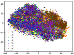
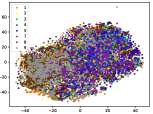
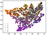
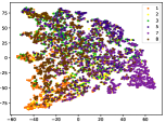
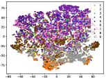
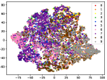
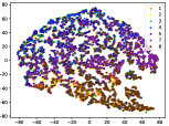
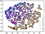
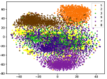
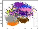
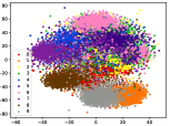
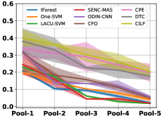
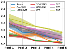
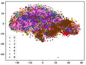
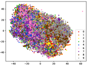
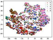
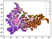
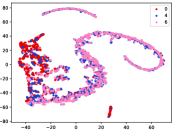
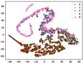
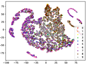
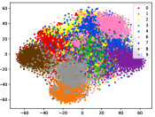
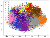
Figure 7 shows feature embedding results within each time window using T-SNE, in which each class randomly samples 800 instances. Similarly, the output of CILF has more distinct groups from different classes compared to other methods, which indicates that CILF can solve the embedding confusion effectively. Table V and Figure 8 compared the forgetting performance of CILF with baseline methods. Identically, the results show that CILF has the least forgetting, and performance of known classes fall slower, which shows that CILF can mitigate forgetting under multiple novel classes scenario.
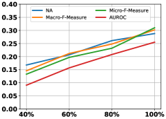
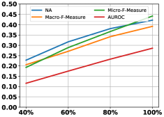
4.7 Influence of Query Size
Figure 9 shows the influence of querying number about potential novel class instances, we only give the results of CIFAR-10 considering page limitation. Here, we randomly query a subset, i.e., a percent of potential instances from the current window. From the figure, it can be observed that the prediction performance improves with the increase of labeled data, which verifies the importance of ground-truths for model update.
(a) Single CIFAR-10
(b) Multiple CIFAR-10
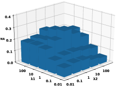
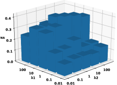
4.8 Parameter Sensitivity
The main parameters in novel class detection and model update are the and in Eq. 10. We vary these parameters in to study its sensitivity to classification performance and record the AUROC results in figure 10. Both the single and multiple cases indicate that the performances are higher when setting with a larger value, i.e., larger than 1.
(c) Multiple CIFAR-10
(d) Multiple CIFAR-50
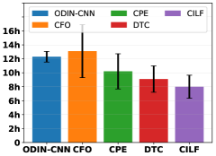
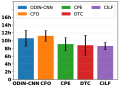
4.9 Execution Time for Model Update
Consider our method focuses on multiple novel class detection, thus we analyze execution time for detecting and updating model with multiple novel class case. In detail, we select the five deep methods, i.e. ODIN-CNN, CFO, CPR, DTC and CILF, and record the results of multiple novel class case in Figure 11. CILF achieves the fastest results, this is because other methods require additional clustering operations, and embedding confusion will slow down the clustering convergence, which indicates the curriculum clustering can accelerate detection.
5 Conclusion
Real-word application always receive the data in stream form, which emerges previously unknown classes sequentially. Incremental NCD has two main challenges: 1) Novel class detection, streaming test data will accept unknown classes; 2) Model expansion, the model needs to be effectively updated after the new class detection. However, traditional methods have not always fully considered these two challenges. To this end, we propose a Class-Incremental Learning without Forgetting (CILF) framework. CILF designed to regularize classification with decoupled prototype based loss, which can improve the intra-class and inter-class structure significantly, and acquire a compact embedding representation for novel class detection in result. Then, CILF employed a learnable curriculum clustering operator to estimate the number of semantic clusters via fine-tuning the learned network. Last, CILF updates the network effectively with robust regularization to mitigate the catastrophic forgetting. Consequently, empirical studies showed the superior performances of CILF.
References
- Masi et al. [2018] I. Masi, Y. Wu, T. Hassner, and P. Natarajan, “Deep face recognition: A survey,” in Proceedings of the 31st SIBGRAPI Conference on Graphics, Patterns and Images, Parana, Brazil, 2018, pp. 471–478.
- Schmarje et al. [2020] L. Schmarje, M. Santarossa, S.-M. Schroder, and R. Koch, “A survey on semi-, self- and unsupervised techniques in image classification,” CoRR, vol. abs/2002.08721, 2020.
- Palatucci et al. [2009] M. Palatucci, D. Pomerleau, G. E. Hinton, and T. M. Mitchell, “Zero-shot learning with semantic output codes,” in Advances in Neural Information Processing Systems 22, Vancouver, British Columbia, 2009, pp. 1410–1418.
- Fu et al. [2018] Y. Fu, T. Xiang, Y.-G. Jiang, X. Xue, L. Sigal, and S. Gong, “Recent advances in zero-shot recognition: Toward data-efficient understanding of visual content,” IEEE Signal Process. Mag., vol. 35, no. 1, pp. 112–125, 2018.
- Min et al. [2019] S. Min, H. Yao, H. Xie, Z.-J. Zha, and Y. Zhang, “Domain-specific embedding network for zero-shot recognition,” in Proceedings of the 27th ACM International Conference on Multimedia, Nice, France, 2019, pp. 2070–2078.
- Lampert et al. [2014] C. H. Lampert, H. Nickisch, and S. Harmeling, “Attribute-based classification for zero-shot visual object categorization,” IEEE Trans. Pattern Anal. Mach. Intell., vol. 36, no. 3, pp. 453–465, 2014.
- Changpinyo et al. [2016] S. Changpinyo, W.-L. Chao, B. Gong, and F. Sha, “Synthesized classifiers for zero-shot learning,” in Proceedings of the 2016 IEEE Conference on Computer Vision and Pattern Recognition, Las Vegas, NV, 2016, pp. 5327–5336.
- Li et al. [2019] J. Li, M. Jing, K. Lu, L. Zhu, Y. Yang, and Z. Huang, “Alleviating feature confusion for generative zero-shot learning,” in Proceedings of the 27th ACM International Conference on Multimedia, Nice, France, 2019, pp. 1587–1595.
- Bendale and Boult [2016] A. Bendale and T. E. Boult, “Towards open set deep networks,” in Proceedings of the 2016 IEEE Conference on Computer Vision and Pattern Recognition, Las Vegas, NV, 2016, pp. 1563–1572.
- Hassen and Chan [2018] M. Hassen and P. K. Chan, “Learning a neural-network-based representation for open set recognition,” CoRR, vol. abs/1802.04365, 2018.
- Ge et al. [2017] Z. Ge, S. Demyanov, and R. Garnavi, “Generative openmax for multi-class open set classification,” in Proceedings of the British Machine Vision Conference, London, UK, 2017.
- Jo et al. [2018] I. Jo, J. Kim, H. Kang, Y. Kim, and S. Choi, “Open set recognition by regularising classifier with fake data generated by generative adversarial networks,” in Proceedings of the 2018 IEEE International Conference on Acoustics, Speech and Signal Processing, Calgary, Canada, 2018, pp. 2686–2690.
- Neal et al. [2018] L. Neal, M. L. Olson, X. Z. Fern, W.-K. Wong, and F. Li, “Open set learning with counterfactual images,” in Proceedings of the 15th European Conference Computer Vision, Munich, Germany, 2018, pp. 620–635.
- Ratcliff [1990] R. Ratcliff, “Connectionist models of recognition memory: constraints imposed by learning and forgetting functions.” Psychol. Review, vol. 97, no. 2, p. 285, 1990.
- Rebuffi et al. [2017] S.-A. Rebuffi, A. Kolesnikov, G. Sperl, and C. H. Lampert, “icarl: Incremental classifier and representation learning,” in Proceedings of the 2017 IEEE Conference on Computer Vision and Pattern Recognition, Honolulu, HI, 2017, pp. 5533–5542.
- Isele and Cosgun [2018] D. Isele and A. Cosgun, “Selective experience replay for lifelong learning,” in Proceedings of the 32nd AAAI Conference on Artificial Intelligence, New Orleans, Louisiana, 2018, pp. 3302–3309.
- Wang et al. [2019] Z. Wang, Z. Kong, S. Chandra, H. Tao, and L. Khan, “Robust high dimensional stream classification with novel class detection,” in Proceedings of the 35th IEEE International Conference on Data Engineering, Macao, China, 2019, pp. 1418–1429.
- Nguyen et al. [2017] C. V. Nguyen, Y. Li, T. D. Bui, and R. E. Turner, “Variational continual learning,” CoRR, vol. abs/1710.10628, 2017.
- Da et al. [2014] Q. Da, Y. Yu, and Z.-H. Zhou, “Learning with augmented class by exploiting unlabeled data,” in Proceedings of the 28th AAAI Conference on Artificial Intelligence, Quebec, Canada, 2014, pp. 1760–1766.
- Mu et al. [2017] X. Mu, F. Zhu, J. Du, E.-P. Lim, and Z.-H. Zhou, “Streaming classification with emerging new class by class matrix sketching,” in Proceedings of the 31st AAAI Conference on Artificial Intelligence, San Francisco, California, 2017, pp. 2373–2379.
- Hendrycks and Gimpel [2017] D. Hendrycks and K. Gimpel, “A baseline for detecting misclassified and out-of-distribution examples in neural networks,” in Proceedings of the 5th International Conference on Learning Representations, Toulon, France, 2017.
- Liang et al. [2018] S. Liang, Y. Li, and R. Srikant, “Enhancing the reliability of out-of-distribution image detection in neural networks,” in Proceedings of the 6th International Conference on Learning Representations, Vancouver, Canada, 2018.
- Hsu et al. [2019] Y. Hsu, Z. Lv, J. Schlosser, P. Odom, and Z. Kira, “Multi-class classification without multi-class labels,” in Proceedings of the 7th International Conference on Learning Representations, New Orleans, LA, 2019.
- Han et al. [2019] K. Han, A. Vedaldi, and A. Zisserman, “Learning to discover novel visual categories via deep transfer clustering,” in Proceedings of the 2019 IEEE International Conference on Computer Vision, Seoul, Korea, 2019, pp. 8400–8408.
- jun Zhang et al. [2016] L. jun Zhang, T. Yang, R. Jin, Y. Xiao, and Z.-H. Zhou, “Online stochastic linear optimization under one-bit feedback,” in Proceedings of the 31sh International Conference Machine Learning, New York City, NY, 2016, pp. 392–401.
- Lopez-Paz and Ranzato [2017] D. Lopez-Paz and M. Ranzato, “Gradient episodic memory for continual learning,” in Advances in Neural Information Processing Systems 30, Long Beach, CA, 2017, pp. 6467–6476.
- Li and Hoiem [2016] Z. Li and D. Hoiem, “Learning without forgetting,” in Proceedings of the 14th European Conference Computer Vision, Amsterdam, The Netherlands, 2016, pp. 614–629.
- Kirkpatrick et al. [2016] J. Kirkpatrick, R. Pascanu, N. C. Rabinowitz, J. Veness, G. Desjardins, A. A. Rusu, K. Milan, J. Quan, T. Ramalho, A. Grabska-Barwinska, D. Hassabis, C. Clopath, D. Kumaran, and R. Hadsell, “Overcoming catastrophic forgetting in neural networks,” CoRR, vol. abs/1612.00796, 2016.
- Lee et al. [2017a] S.-W. Lee, J.-H. Kim, J. Jun, J.-W. Ha, and B.-T. Zhang, “Overcoming catastrophic forgetting by incremental moment matching,” in NIPS, Long Beach, CA, 2017, pp. 4655–4665.
- Geng et al. [2018] C. Geng, S.-J. Huang, and S. Chen, “Recent advances in open set recognition: A survey,” CoRR, vol. abs/1811.08581, 2018.
- Kulis [2013] B. Kulis, “Metric learning: A survey,” Foundations and Trends in Machine Learning, vol. 5, no. 4, pp. 287–364, 2013.
- Bishop and Nasrabadi [2007] C. M. Bishop and N. M. Nasrabadi, “Pattern recognition and machine learning,” J. Electronic Imaging, vol. 16, no. 4, p. 049901, 2007.
- Liu et al. [2016] W. Liu, Y. Wen, Z. Yu, and M. Yang, “Large-margin softmax loss for convolutional neural networks,” in Proceedings of the 33nd International Conference on Machine Learning, New York City, NY, 2016, pp. 507–516.
- Laine and Aila [2017] S. Laine and T. Aila, “Temporal ensembling for semi-supervised learning,” in Proceedings of the 5th International Conference on Learning Representations, Toulon, France, 2017.
- Yu and Tao [2019] B. Yu and D. Tao, “Deep metric learning with tuplet margin loss,” in Proceedings of the 2019 IEEE International Conference on Computer Vision, Seoul, Korea, 2019, pp. 6489–6498.
- Bengio et al. [2009] Y. Bengio, J. Louradour, R. Collobert, and J. Weston, “Curriculum learning,” in Proceedings of the 26th Annual International Conference on Machine Learning, Montreal, Canada, 2009, pp. 41–48.
- Hacohen and Weinshall [2019] G. Hacohen and D. Weinshall, “On the power of curriculum learning in training deep networks,” in Proceedings of the 36th International Conference on Machine Learning, Long Beach, California, 2019, pp. 2535–2544.
- Dhillon et al. [2007] I. S. Dhillon, Y. Guan, and B. Kulis, “Weighted graph cuts without eigenvectors A multilevel approach,” IEEE Trans. Pattern Anal. Mach. Intell., vol. 29, no. 11, pp. 1944–1957, 2007.
- Arbelaitz et al. [2013] O. Arbelaitz, I. Gurrutxaga, J. Muguerza, J. M. Perez, and I. Perona, “An extensive comparative study of cluster validity indices,” Pattern Recognit., vol. 46, no. 1, pp. 243–256, 2013.
- Haque et al. [2016] A. Haque, L. Khan, and M. Baron, “SAND: semi-supervised adaptive novel class detection and classification over data stream,” in Proceedings of the 30th AAAI Conference on Artificial Intelligence, Phoenix, Arizona, 2016, pp. 1652–1658.
- LeCun et al. [1998] Y. LeCun, C. Cortes, and C. J. Burges, “The mnist database of handwritten digits, 1998,” URL http://yann. lecun. com/exdb/mnist, vol. 10, p. 34, 1998.
- Krizhevsky et al. [2009] A. Krizhevsky, G. Hinton et al., “Learning multiple layers of features from tiny images,” 2009.
- Masud et al. [2011] M. M. Masud, J. Gao, L. Khan, J. Han, and B. M. Thuraisingham, “Classification and novel class detection in concept-drifting data streams under time constraints,” IEEE Trans. Knowl. Data Eng., vol. 23, no. 6, pp. 859–874, 2011.
- Chaudhry et al. [2018] A. Chaudhry, P. K. Dokania, T. Ajanthan, and P. H. Torr, “Riemannian walk for incremental learning: Understanding forgetting and intransigence,” CoRR, vol. abs/1801.10112, 2018.
- Liu et al. [2008] F. T. Liu, K. M. Ting, and Z. Zhou, “Isolation forest,” in Proceedings of the 8th IEEE International Conference on Data Mining, Pisa, Italy, 2008, pp. 413–422.
- Lee et al. [2017b] J. Lee, J. Yoon, E. Yang, and S. J. Hwang, “Lifelong learning with dynamically expandable networks,” CoRR, vol. abs/1708.01547, 2017.
- Junior et al. [2017] P. R. M. Junior, R. M. de Souza, R. de Oliveira Werneck, B. V. Stein, D. V. Pazinato, W. R. de Almeida, O. A. B. Penatti, R. da Silva Torres, and A. Rocha, “Nearest neighbors distance ratio open-set classifier,” Mach. Learn., vol. 106, no. 3, pp. 359–386, 2017.
- He et al. [2016] K. He, X. Zhang, S. Ren, and J. Sun, “Deep residual learning for image recognition,” in Proceedings of the 2016 IEEE Conference on Computer Vision and Pattern Recognition, Las Vegas, NV, 2016, pp. 770–778.
- Sutskever et al. [2013] I. Sutskever, J. Martens, G. E. Dahl, and G. E. Hinton, “On the importance of initialization and momentum in deep learning,” in ICML, 2013, pp. 1139–1147.
- Maaten and Hinton [2008] L. v. d. Maaten and G. Hinton, “Visualizing data using t-sne,” Journal of machine learning research, vol. 9, no. Nov, pp. 2579–2605, 2008.
![[Uncaptioned image]](https://cdn.awesomepapers.org/papers/8df2a303-7b02-4495-8670-036749f4f76b/yangy.jpg) |
Yang Yang received the Ph.D. degree in computer science, Nanjing University, China in 2019. At the same year, he became a faculty member at Nanjing University of Science and Technology, China. He is currently a Professor with the Computer Science and Engineering. His research interests lie primarily in machine learning and data mining, including heterogeneous learning, model reuse, and incremental mining. He serves as PC in leading conferences such as IJCAI, AAAI, ICML, NIPS, etc. |
![[Uncaptioned image]](https://cdn.awesomepapers.org/papers/8df2a303-7b02-4495-8670-036749f4f76b/sunzq.jpg) |
Zhen-Qiang Sun is working towards the M.Sc. degree with the School of Computer Science Technology in Nanjing Normal University, China. His research interests lie primarily in machine learning and data mining, including incremental learning. |
![[Uncaptioned image]](https://cdn.awesomepapers.org/papers/8df2a303-7b02-4495-8670-036749f4f76b/yanjf.jpg) |
Yanjie Fu received the BE degree from the University of Science and Technology of China, in 2008, the ME degree from the Chinese Academy of Sciences, in 2011, and the PhD degree from Rutgers University, in 2016. He is currently an assistant professor with the Missouri University of Science and Technology. His general interests are data mining and big data analytics. He has published prolifically in refereed journals and conference proceedings, such as the IEEE Transactions on Knowledge and Data Engineering, the ACM Transactions on Knowledge Discovery from Data, the IEEE Transactions on Mobile Computing, and ACM SIGKDD. |
![[Uncaptioned image]](https://cdn.awesomepapers.org/papers/8df2a303-7b02-4495-8670-036749f4f76b/zhuhs.jpg) |
HengShu Zhu (SM’19) is currently a principal data scientist architect at Baidu Inc. He received the Ph.D. degree in 2014 and B.E. degree in 2009, both in Computer Science from University of Science and Technology of China (USTC), China. His general area of research is data mining and machine learning, with a focus on developing advanced data analysis techniques for innovative business applications. He has published prolifically in refereed journals and conference proceedings, including IEEE Transactions on Knowledge and Data Engineering (TKDE), IEEE Transactions on Mobile Computing (TMC), ACM Transactions on Information Systems (ACM TOIS), ACM Transactions on Knowledge Discovery from Data (TKDD), ACM SIGKDD, ACM SIGIR, WWW, IJCAI, and AAAI. He has served regularly on the organization and program committees of numerous conferences, including as a program co-chair of the KDD Cup-2019 Regular ML Track, and a founding co-chair of the first International Workshop on Organizational Behavior and Talent Analytics (OBTA) and the International Workshop on Talent and Management Computing (TMC), in conjunction with ACM SIGKDD. He was the recipient of the Distinguished Dissertation Award of CAS (2016), the Distinguished Dissertation Award of CAAI (2016), the Special Prize of President Scholarship for Postgraduate Students of CAS (2014), the Best Student Paper Award of KSEM-2011, WAIM-2013, CCDM-2014, and the Best Paper Nomination of ICDM-2014. He is the senior member of IEEE, ACM, and CCF. |
![[Uncaptioned image]](https://cdn.awesomepapers.org/papers/8df2a303-7b02-4495-8670-036749f4f76b/xiongh.jpg) |
Hui Xiong (SM’07) is currently a Full Professor at the Rutgers, the State University of New Jersey, where he received the 2018 Ram Charan Management Practice Award as the Grand Prix winner from the Harvard Business Review, RBS Dean’s Research Professorship (2016), the Rutgers University Board of Trustees Research Fellowship for Scholarly Excellence (2009), the ICDM Best Research Paper Award (2011), and the IEEE ICDM Outstanding Service Award (2017). He received the Ph.D. degree from the University of Minnesota (UMN), USA. He is a co-Editor-in-Chief of Encyclopedia of GIS, an Associate Editor of IEEE Transactions on Big Data (TBD), ACM Transactions on Knowledge Discovery from Data (TKDD), and ACM Transactions on Management Information Systems (TMIS). He has served regularly on the organization and program committees of numerous conferences, including as a Program Co-Chair of the Industrial and Government Track for the 18th ACM SIGKDD International Conference on Knowledge Discovery and Data Mining (KDD), a Program Co-Chair for the IEEE 2013 International Conference on Data Mining (ICDM), a General Co-Chair for the IEEE 2015 International Conference on Data Mining (ICDM), and a Program Co-Chair of the Research Track for the 2018 ACM SIGKDD International Conference on Knowledge Discovery and Data Mining. He is an IEEE Fellow and an ACM Distinguished Scientist. |
![[Uncaptioned image]](https://cdn.awesomepapers.org/papers/8df2a303-7b02-4495-8670-036749f4f76b/yangj.jpg) |
Jian Yang (M’08) received the Ph.D. degree in pattern recognition and intelligence systems from the Nanjing University of Science and Technology (NUST), Nanjing, China, in 2002. In 2003, he was a Post-Doctoral Researcher with the University of Zaragoza, Zaragoza, Spain. From 2004 to 2006, he was a Post-Doctoral Fellow with the Biometrics Centre, The Hong Kong Polytechnic University, Hong Kong. From 2006 to 2007, he was a Post-Doctoral Fellow with the Department of Computer Science, New Jersey Institute of Technology, Newark, NJ, USA. He is currently a Chang-Jiang Professor with the School of Computer Science and Engineering, NUST. He has authored more than 200 scientific papers in pattern recognition and computer vision. His papers have been cited more than 6000 times in the Web of Science and 15,000 times in the Scholar Google. His current research interests include pattern recognition, computer vision, and machine learning. Dr. Yang is a Fellow of IAPR. He is currently an Associate Editor of Pattern Recognition, Pattern Recognition Letters, the IEEE TRANSACTIONS ON NEURAL NETWORKS AND LEARNING SYSTEMS, and Neurocomputing. |