Layph: Making Change Propagation Constraint in Incremental Graph Processing by Layering Graph
Abstract
Real-world graphs are constantly evolving, which demands updates of the previous analysis results to accommodate graph changes. By using the memoized previous computation state, incremental graph computation can reduce unnecessary recomputation. However, a small change may propagate over the whole graph and lead to large-scale iterative computations. To address this problem, we propose Layph, a two-layered graph framework. The upper layer is a skeleton of the graph which is much smaller than the original graph, and the lower layer has some disjoint subgraphs. Layph limits costly global iterative computations on the original graph to the small graph skeleton and a few subgraphs updated with the input graph changes. In this way, many vertices and edges are not involved in iterative computations, which significantly reduces the computation overhead and improves the performance of incremental graph processing. Our experimental results show that Layph outperforms current state-of-the-art incremental graph systems by on average (up to ) in response time.
Index Terms:
incremental graph processing, layered graph, graph skeletonI Introduction
Iterative graph algorithms, e.g., single source shortest path () and , have been widely applied in many fields [1, 2, 3, 4, 5]. Real-world graphs are continuously evolving with structure changes, where vertices and edges are inserted or deleted arbitrarily. These changes are usually small, e.g., there were 6.4 million articles on English Wikipedia in [6], but the average number of new articles per day was only . Traditional classical graph processing systems [7, 8, 9, 10, 11, 12, 13] have to recompute the updated graph from scratch. However, there are considerable overlaps between computations before and after the graph updates. It is desirable to adopt incremental graph computation to cope with these small changes efficiently. That is, a batched iterative algorithm is applied to compute the result over the original graph till convergence, and then an incremental algorithm is used to adjust the result in response to the input changes to .


The incremental graph computation can reduce unnecessary recomputation by using the memoized iterative computation state, e.g., intermediate vertex states or messages. The benefits of incremental graph computation have led to the development of many incremental graph processing systems, such as KickStarter [14], GraphBolt [15], Ingress [16], DZiG [17], and RisGraph [18]. They memoize (intermediate or final) vertex states and organize them in a data structure that captures result dependencies, such as a tree (for critical path) [14], [18] or a multilayer network (for per-iteration dependencies) [15], [17]. With such a structure, the update of a vertex/edge will be propagated for updating the memoized intermediate/final states of vertices iteratively. However, an upstream vertex/edge update may incur a large number of updates to the downstream vertex/edge states in existing incremental graph processing systems. That is, a small change may propagate over the entire graph and lead to large-scale iterative computations.
With 5000 random edge updates on the UK graph (see Table I for details), we run and on five state-of-the-art incremental graph processing systems (KickStarter [14], GraphBolt [15], DZiG [17], RisGraph [18], and Ingress [16]) and a Restart system that starts computations on the updated graph from scratch. The number of edge activations and runtime of these systems are reported in Figure 1. Even though the amount of updates is small (), these updates propagate widely and iteratively on the graph, resulting in a large number of edge activations in some systems, which is almost approaching the number in restarting iterative computations.

We empirically illustrate this observation with an example in Figure 2. Figure 2b shows an updated graph based on graph , where the edge (, ) is deleted and a new edge (, ) is added. As shown in Figure 2c, when running , existing incremental graph processing systems [14, 16, 18] activate most of the vertices and edges. As the iteration proceeds, the activated vertices may be updated several times, e.g., and its downstream vertices are updated twice due to the update messages from at different iterations.
Challenge. Based on the above observations and illustration, we can see that very small graph changes can also lead to a large number of iterative computations, even on the basis of previous memoized vertex/edge states provided by incremental processing systems. The main reason is that, in real-world graphs, vertices are either directly or indirectly connected in several hops, which makes it hard to constrain the affected area. The native properties of real graphs fundamentally limit the effectiveness of incremental graph computation. Is it possible to reconstruct the graph structure to boost the performance of incremental graph computation?
Intuition. In incremental graph computation, the messages initiated by graph updates are propagated iteratively to update the states of vertices. When an update message enters into a dense subgraph from entry vertices, a large number of internal vertices and edges within the subgraph will be activated and involved in the iterative computation. The incoming messages probably require many iterations to get out of this dense subgraph from exit vertices. A natural idea is to extract the entry and exit vertices of the dense subgraph, and construct shortcuts between them to propagate messages directly through the dense subgraph, which can avoid the activations of a large number of internal vertices and edges. As shown in Figure 2d, we extract the entry vertex and exit vertex of and construct a shortcut between them. Then the messages can be propagated directly through via the shortcut. Furthermore, we construct a shortcut between the entry vertices and the internal vertices in each subgraph. The entry vertices can accumulate the incoming messages and eventually assign them to the internal vertices at a time via the shortcuts. As shown in Figure 2d, after accumulates all incoming messages, will send the update messages to - at a time. In this way, only the entry and exit vertices of subgraphs and outliers participate in the global iterative computations.
Our Solution. Based on the above intuition, we propose an incremental graph processing framework by layering the graph, . As shown in Figure 2d, divides the graph into two layers, the upper layer () and the lower layer (). is a skeleton of the original graph composed of the boundary vertices of subgraphs and outliers, the size of which is much smaller than that of . is composed of some disjoint subgraphs. Vertices on and vertices on are connected by shortcuts (dashed lines) or edges. After is updated by , we first update the layered graph accordingly. The revision messages are generated and propagated only within the subgraphs on that are updated by . As shown in Figure 2e, revision messages are generated from and are propagated within . Then the messages are uploaded to , e.g., the messages are propagated from to in Figure 2e. The global iterative computations are performed on . Compared with 10 edges participating in the iterative computation in Figure 2c, only 2 edges/shortcuts are involved on in Figure 2e. Therefore, the global iterative computations on are much faster than that on graph . Finally, the updates are assigned to the other subgraphs on , e.g., . Vertex states are updated directly through shortcuts without iterative computations. We can see that performs iterative computations only on the upper layer small skeleton and a few subgraphs (on ) that are updated by . Most vertices and edges on are not involved in iterative computations. Thus is able to accelerate the incremental graph computation efficiently.
To sum up, we make the following contributions.
- •
-
•
Effective Skeleton Extraction and Automated Shortcut Deduction. We design an effective skeleton extraction method that reduces the size of the skeleton by replicating vertices. Based on the input vertex-centric program, our proposed framework can deduce the weight of shortcuts automatically. (Section IV)
-
•
High-Performance Runtime Engine. We implement our runtime engine based on Ingress [16] and Alibaba’s libgrape-lite [19]. Comparing with current state-of-the-art incremental graph processing systems, can achieve 3.13-15.82 speedup over Kickstarter [14], 2.54-8.49 speedup over RisGraph [18], 2.99-36.66 speedup over GraphBolt [15], 2.92-32.93 speedup over DZiG [17], and 1.06-7.22 speedup over Ingress [16]. (Section VI)
II Preliminaries
This section provides the necessary preliminaries for iterative graph computation and incremental graph computation.
II-A Iterative Graph Computation
Given an input graph , where is a finite set of vertices and is a set of edges. The weight of each edge is in a weighted graph or a consistent value 1 in an unweighted graph. In general, an iterative graph algorithm that executes in an accumulative model, includes two types of operations, i.e., message generation and message aggregation [9, 10, 20].
| (1) | ||||
where .
The message generate operation applied on each vertex prepares the message for each outgoing edge based on the aggregation of received message and the edge weight . The aggregation operation is applied on each destination vertex . It first aggregates the messages that terminate at to obtain a new message , then aggregates the old vertex state and the aggregated message to update the vertex state . The two-step process is applied iteratively till convergence (when vertex states become stable). To sum up, an iterative graph computation can be expressed as where and are the operations that specify the algorithm logic, and and are the initial values of vertex states and root messages respectively. A graph computation on the input graph can be denoted as .
Suppose can be executed asynchronously, then it can be expressed as Equation (1) naturally, such as . Otherwise, the synchronous algorithms should be rewritten in accumulative mode and executed asynchronously, such as PageRank. There are some efforts [10, 9] that rewrite a synchronous algorithm in asynchronous accumulative mode.
Example 1: We show two example algorithms.
(a) . computes the shortest distance from a given source to all vertices in a directed and weighted graph . is represented as follows
-
•
; ;
-
•
if , otherwise ;
-
•
if , otherwise .
Here the state of indicates the shortest distance from source to and represents the length of the edge . Initially, we have for , and for all . Each vertex generates and sends a message to each neighbor , which represents the current shortest distance from the source. Each destination vertex aggregates the messages from its incoming neighbors and updates its state by . The algorithm terminates when the shortest distance values of all vertices are not changed.
(b) . computes the set of ranking scores . Here is a constant damping factor and denotes the number of outgoing neighbors of . Different from the original algorithm that exploits the power method, an asynchronous algorithm [10] that has been proved to be equivalent to the original can be represented as follows
-
•
;
-
•
, ; , .
Intuitively, each vertex uses its state to store its score. Initially, we have and for all . Every time when a vertex receives a message , it will send to each neighbor . Each neighbor aggregates the messages from its incoming neighbors by and updates its state by accumulating the aggregated messages. The algorithm terminates when all vertex states are stable.
Equation (1) defines the vertex-centric format of asynchronous iterative computation. On this basis, we can define a set-based iterative computation as follows
| (2) | ||||
is the set of vertex states. is the set of root messages of each vertex and is the set of generated messages on all edges. It should be noticed that these are slight meaning changes of and in set-based format. is the message generate operation with edge information embedded so it only needs a single parameter . is the group-by aggregator (group by vertex id). Based on this set-based computation, the vertex states set after iterations is
| (3) | ||||
where and denotes applications of .
Message Passing’s Perspective. From message propagation’s perspective, the final state of each vertex is obtained by accumulating the messages initiated from all vertices transferred along different paths. In each iteration, i.e., one time application of and , a message is processed and split into several messages from a vertex to its direct neighbors (under the effect of ). The messages received from different incoming neighbors are aggregated into one message (under the effect of ), which will be propagated again in the next iteration. At the same time, the aggregated message is applied to the vertex state (under the effect of ). This is exactly the process described in Equation (1).
II-B Incremental Graph Computation
Given an iterative graph computation and its incremental counterpart , the problem of incremental computation arises when the input graph is updated with . Let denote the output of an old graph with the effect of batch graph algorithm . The inputs of incremental computation include and graph updates . Then we have
| (4) |
It means that the incremental computation that is performed based on the old result and the graph updates is expected to output , where denotes applying the updates to . It is noticeable that the incrementalization scheme is algorithm-specific and is deduced from its original algorithm .
The input batch update consists of a set of unit updates. To simplify our discussion, we consider the insertion or deletion of a single edge as a unit update in a sequence, which can simulate certain modifications. For instance, each change to an edge weight can be considered as deleting the edge and followed by adding another edge with the new property. The incremental computation will identify the changes to the old output and make corrections of the previous computation in response to .
Message Passing’s Perspective. From Equation (3) we know that the input changes will affect the message propagation since both and are correlated with the graph structure, and as a result, will change the final vertex states. Due to the insertion, update, or deletion of an edge, a set of messages might become invalid, and another set of messages might be missing. An old message transmitted during the run over the original graph is called invalid if the path for passing the message disappears due to input updates . A new message transferred in the run over the is called missing if it did not appear in the run over . In incremental computation, we should first discover all the invalid and missing messages and then perform the corrections on the affected areas of by generating cancellation messages (resp. compensation messages) to retract (resp. replay) effects of the invalid messages (resp. missing messages) [14, 16, 15, 17]. In this paper, the cancellation and compensation messages are collectively called as revision messages.
III Framework Overview

In this section, we first present the workflow of the layered graph framework and then analyze the benefits of .
Workflow of Layph. The overall workflow is illustrated in Figure 3. At the beginning of incremental graph processing, given a graph , we first divide the graph into two layers. The upper layer () is the skeleton of the graph. consists of the entry/exit vertices of all dense subgraphs, vertices that are not in any dense subgraph, and the shortcuts or edges between them. The lower layer () is composed of all disjointed dense subgraphs. The entry vertices (on ) and the internal vertices (on ) of each dense subgraph are connected with shortcuts between and . Please refer to Section IV for the details of constructing the layered graph. Then we perform incremental graph computations on the layered graph, which includes two steps, i) the layered graph update (Section IV) and ii) the vertex states update (Section V).
Layered Graph Update. Given a layered graph of an original graph , should be updated, when is updated by . This is because the shortcuts, including the shortcuts on and the shortcuts between and , may be changed as the graph changes. The shortcut update requires iterative computations and is only performed on the subgraphs updated by . Meanwhile, the shortcut update can be parallelized well as the subgraphs are independent of each other.
Vertex States Update. When the graph changes, we first deduce the revision messages based on the memoized information [16, 14, 15], then propagate the revision messages on the layered graph to revise the vertex states. The incremental computation on is performed as follows.
-
•
Revision messages upload. In order to apply the revision messages deduced by vertices on to vertices on , the revision messages on should be uploaded to . Similar to shortcut updates, the messages upload can also be performed in parallel and only performed on subgraphs affected by .
-
•
Iterative computation on . After receiving the revision messages from , iterative computations are performed to propagate the revision messages and revise the states of the vertices on .
-
•
Revision messages assignment. After the iterative computations on , the entry vertices (on ) of each subgraph accumulate all the revision messages. The accumulated revision messages are assigned from entry vertices to internal vertices (on ) through shortcuts to revise the states of vertices on .
Analysis. From the above workflow of , we can see that the iterative computations only perform on and a few subgraphs on . The vertices and edges within subgraphs that are not updated by are not involved in iterative computations, which saves significant computation overhead.
IV Layered Graph Construction And Update
is performed on a layered graph. This section presents how to construct a layered graph and update it incrementally.
IV-A Layered Graph Construction
In this section, we first introduce how to extract vertices on the upper layer. Then we provide an automated shortcut calculation method.
IV-A1 Upper Layer Vertices Extraction
As we have presented the intuition behind in Section I and the workflow in Section III, we should extract the entry and exit vertices of the dense subgraphs and the vertices that are not in any subgraphs into the upper layer to construct the skeleton of the graph. This requires us to discover all the dense subgraphs from the original graph. Before introducing the method of dense subgraph discovery, we first provide the formal definition of entry/exit/internal vertices and dense subgraph.
Definition 1 (Entry/Exit/Internal Vertices).
Given a subgraph of the graph , where and . The entry vertices of are defined as , the exit vertices of are defined as , and the internal vertices of are defined as .
Definition 2 (Dense Subgraph).
Given an input graph , the subgraph of is a dense subgraph such that the product of the number of entry vertices and that of exit vertices is smaller than the number of edges in , i.e., .
Our definition of the dense subgraph is based on the following observation. For each entry vertex of subgraph , it is required to connect with all exit vertices using shortcuts. Thus, the number of the shortcuts in is the product of the number of entry and exit vertices, i.e., . If there are only a few edges in , e.g., , then propagating messages from entry to exit vertices through the shortcuts is slower than that through the edges in , because more shortcuts result in more message generation operations and aggregation operations.
From Definition 2, a dense subgraph requires as many internal edges as possible and as few boundary (entry/exit) vertices as possible. We found that the requirements of a dense subgraph are similar to that of the community. The community requires as many internal edges as possible and as few external edges as possible. This inspired us to adopt a community discovery algorithm to discover dense subgraphs. Therefore, in this paper, we use the community discovery algorithm to find dense subgraphs, such as Louvain [21]. However, the community discovery algorithms may find extremely large subgraphs, which decreases the performance of our system since extremely large graphs may result in an imbalance workload. Therefore, we add a threshold to limit the size of each subgraph when discovering the subgraphs, i.e., the number of vertices in each subgraph is smaller than . As a rule of thumb, is set around 0.002-0.2% of the total number of vertices. We also employ the work stealing technique to handle the imbalance workload, in which an idle processing thread will actively search out work for it to complete. A community may not be a dense subgraph. We select the dense subgraphs according to Definition 2, i.e., , from the dense subgraphs candidate set discovered by the community discovery algorithm.
After discovering the dense subgraphs, the internal vertices and edges within them are put into the lower layer, the other vertices and edges i.e., entry/exit vertices of subgraphs and the vertices that are not in any dense subgraphs and their edges are extracted into the upper layer.

Problem Study. Although we can discover dense subgraphs by using the above method, it suffers from a key limitation: the shortcuts that need to be established are still numerous due to the massive number of entry/exit vertices. As shown in Figure 4, we find that most boundary vertices (entry/exit vertices) have high degrees and are likely to have many connections to/from other subgraphs, leading to many entry/exit vertices in the target/source subgraphs. For example, vertex is with high out-degree and has 3 out-edges connected to subgraph , leading to 3 entry vertices in subgraph , and vertex with a high in-degree and has 3 in-edges originating from subgraph , leading to 3 exit vertices in subgraph . A large number of entry/exit vertices incurs a large skeleton of the upper layer as shown in Figure 4b, which will hurt the performance of iterative computation and increase the computation cost for shortcut calculations/updates.
Solution: Vertex Replication. Figure 4 demonstrates that there exist some entry/exit vertices in a subgraph that share the same source/target vertex. This inspires us to propose a vertex replication approach for reducing the number of entry/exit vertices and shortcuts. The idea is illustrated in Figure 4c. After dense subgraph discovery, if the number of entry/exit vertices in a subgraph that share the same source/target vertex is larger than a threshold, the source/target vertex (host vertex) will be replicated in subgraph as a proxy vertex . A high-degree vertex could have many proxy vertices in multiple different dense subgraphs. Both entry and exit vertices can have proxy vertices in other dense subgraphs. For example, in Figure 4c, entry vertex has a proxy vertex acting as a new exit vertex in subgraph . Originally, there are 3 exit vertices in subgraph linking to the entry vertex , while now there is only one exit vertex . Exit vertex has a proxy vertex in as a new entry vertex. There are supposed to be 3 entry vertices in all originating from vertex , but now there is only one entry vertex .
By replicating exit or entry vertices between subgraphs, some boundary vertices of dense subgraphs become internal vertices and move from to . The size of the graph skeleton on is greatly reduced.
IV-A2 Shortcuts Calculation
On the upper layer, there are only entry and exit vertices of each subgraph. It is required to connect them with shortcuts for propagating messages from entry vertices to exit vertices correctly and quickly. During the iterative computations on , the entry vertices send messages to exit vertices directly through shortcuts and do not propagate the messages down to internal vertices. In order to revise the states of vertices on , the entry vertices cache these messages that should be propagated to internal vertices, then propagate them down to internal vertices after the iterative computations terminate. However, these messages spread to all internal vertices may require iterative computations. In order to propagate the messages from the entry vertices to internal vertices efficiently, we also connect them with shortcuts.
Based on the above discussion, there are two kinds of shortcuts in the layered graph, 1) the shortcuts from entry vertices to exit vertices of the dense subgraph, and 2) the shortcuts from entry vertices to internal vertices of the dense subgraph. Essentially, both of these shortcuts connect the entry vertices and other vertices of the dense subgraph. Therefore, they can be calculated simultaneously with the same method. Before introducing the shortcut calculation method, we first provide the formal definition of the shortcut.
Definition 3 (Shortcut).
Given a subgraph and the input messages vector arriving at entry vertices , the shortcuts are the direct connections from entry vertices to all vertices , i.e., where is the weight of a shortcut from vertex to vertex , such that
| (5) |
where and indicate the message propagation through the shortcuts and the original edges respectively, and indicates the message aggregation on vertex set .
The shortcut weight from entry vertex to vertex in can be calculated by the following equation
| (6) |
where is the group-by aggregation on vertex , is the unit message. It means that we first initialize a unit message for entry vertex . Then we perform iterative computation on the subgraph to propagate messages from to until all the vertices in no longer receive any messages or the received messages can be ignored. Finally, the aggregated value of messages received by can be treated as the weight of the shortcut from to , i.e., . The unit message should be the identity element of the operation to make initiation. As shown in Example 2, the identity element of ‘+’ is 0. Then, in SSSP, the value of the messages received by originated from is the shortest path from to , i.e., the weight of the shortcut from to . To alleviate the burden of users, can automatically complete the shortcut calculation by invoking the user-defined and functions without the user’s intervention (see II-A).
Example 2: Consider running on the graph as shown in Figure 2a. When computing the shortcuts inside subgraph , a unit message (as the identity element of ‘+’ since containing ‘+’) is input into entry vertex . We iteratively perform to propagate messages and use to aggregate the received messages for each vertex. Finally, as shown in Figure 2d, the aggregated values of the received messages on are respectively, i.e., the weights of shortcuts are .
Finally, we give the formal definition of the layered graph.
Layered Graph. Given an input graph , a set of dense subgraphs , the layered graph is formed by the upper layer , the lower layer and the edges between and , where (resp. ) is the vertex set on the upper layer (resp. the lower layer) and (resp. ) is the edge set on the upper layer (resp. the lower layer).
-
•
Upper layer ().
-
–
Vertex set is composed of the entry and exit vertices of all dense subgraphs and the vertices that are not in any dense subgraphs.
-
–
Edge set is composed of the shortcuts from entry vertices to exit vertices in each dense subgraph and the edges that are not in any dense subgraphs.
-
–
-
•
Low layer ().
-
–
Vertex set is composed of the internal vertices of all dense subgraphs.
-
–
Edge set is composed of the edges within each subgraph, except the edges from internal vertices to entry/exit vertices.
-
–
-
•
Edges between and . is composed of the shortcuts from entry vertices to internal vertices and the edges from internal vertices to entry/exit vertices within each dense subgraph.
The size of the upper layer (with respect to and ) is expected to be much smaller than that of the original graph (with respect to and ). For example, in Figure 2, the upper layer contains 3 vertices and 3 edges/shortcuts, which is smaller than the original graph with 9 vertices and 14 edges.
Analysis. Due to the introduction of shortcuts, will require more space. The additional space overhead includes the shortcuts from entry vertices to all vertices within each subgraph, i.e., , where is the number of entry vertices of subgraph and is the number of all vertices in . In practice, the additional space overhead is always smaller than that of the original graph, as shown in Figure 11a (in Section VI-G).
IV-B Layered Graph Update
The layered graph needs to be updated when is updated with . The vertices may move between the two layers, due to the generation or disappearance of dense subgraphs, e.g., the internal vertices of the newly generated subgraph move from to . In order to avoid the expensive overhead caused by repeated subgraph discovery, we incrementally update the dense subgraphs with incremental community detection methods, such as C-Blondel [22] or DynaMo [23]. In practice, the size of is very small compared with . A small does not have a large effect on existing dense subgraphs. Thus we update the dense subgraphs only when enough are accumulated. However, even a very small can still change the weight of a number of shortcuts of the layered graph.
Shortcuts update. There are three kinds of shortcut updates. i) Deletion. If all of an entry vertex’s in-edges from outside are deleted, i.e., the connections from outside are cut off, this entry vertex will become an internal vertex, and the shortcuts originated from it should be removed. ii) Addition. If an in-edge from outside is added to an internal vertex, this internal vertex will become an entry vertex. The shortcuts from it to other vertices in the subgraph should be calculated. iii) Weight update. If there are addition or deletion edges within a subgraph, the weight of the shortcuts should be updated.
The shortcut is built inside each dense subgraph according to the Definition 3. Moreover, from the Equation (6), we can see that the weight of each shortcut on only depends on the edges and vertices in , and the shortcuts on the different subgraphs are independent of each other. Therefore, we only need to update the shortcuts on the subgraphs affected by , and the shortcuts for each subgraph can be updated in parallel. For the shortcut deletion or addition, they can be done directly within the subgraph by removing or calculating the shortcut. For the weight update, in order to avoid redundant computation, we use an incremental method to update.
According to Equation (6), the weight of the shortcuts is calculated by iterative computations, and the weight of the shortcut from to is equal to the aggregate all the messages received by through all paths from to . After the edge addition or deletion within the dense subgraph, some messages received by may become invalid or missing. Thus, the update of the shortcut can adopt the existing incremental computation methods [16, 15, 14]. The compensation and cancellation messages can be deduced based on the memoized information when calculating the old shortcut. These messages will be used to redo and undo the effect of missing and invalid messages on vertex , in which there are some missing and invalid messages in the received messages of due to the addition and deletion edges within the dense subgraph.
Example 3: Consider running on the updated graph as shown in Figure 2b. Since only changes , the shortcuts related to do not need to be updated. For , the vertices on do not need to change, since only the inner edges change, and the shortcuts can be updated incrementally. Therefore, we can get the weights of the old shortcuts as the initial weights of the new shortcuts, i.e., the initial values of are set to . Since the edge is deleted and the state of depends on , it is necessary to generate a cancellation message ( means the vertex needs to be reset to the default state, i.e., for ), and sets the state of to [14, 16, 18]. Meantime, will get a message from its neighbor . In addition, since the edge is added, it is necessary to generate a compensation message . Then all these revision messages will be propagated inside . Finally, as shown in Figure 2e, the aggregated values of the received messages on are respectively, i.e., the new weights of the shortcuts are .
V Incremental processing with Layered Graph
This section will introduce how performs incremental graph processing on the layered graph.
Revision messages deduction. As shown in Equation (3), the final vertex state is determined by the received messages that are from ALL vertices and transferred along different paths. When the graph is updated, the messages received by vertices may change due to the changes in the paths that messages propagate. The incremental graph processing framework can automatically [14, 16] or manually [15, 17] obtain the revision messages i.e., compensation messages and cancellation messages, and propagate them to revise the effect of the missing and invalid messages on vertex states [16, 15]. For the revision messages, we can deduce them by employing the method proposed in our previous work [16].
After deducing the revision messages, we propagate them efficiently with the help of . As we have introduced in Section III, the propagation of revision messages on is in three steps, 1) messages upload, 2) iterative computation, and 3) messages assignment.
V-A Messages Upload
The upper layer only contains a subset of vertices, and the internal vertices inside each subgraph on do not participate in iterative computation on . To ensure that all vertices on converge with the effects of internal vertices, the iterative computation on should collect not only the revision messages deduced by the vertices on but also those by internal vertices. Thus, it is required to upload the revision messages deduced by the internal vertices of the dense subgraphs on to . Since the entry/exit vertices of each dense subgraph are on , messages upload can be done by propagating the revision messages to entry/exit vertices.
Not all the internal vertices within each dense subgraph have connections with the entry/exit vertices, thus, we perform a local iterative computation to propagate internal revision messages to the entry/exit vertices of the subgraph. The iterative computation terminates when the messages received by entry/exit vertices can be ignored. After the upload of the messages, the accumulated messages on the entry vertices and exit vertices can be treated as their initial revision messages i.e.,, . Together with the initial messages of vertices that are not in any dense subgraph on , i.e., , the initial messages of vertices on can be expressed as follows
| (7) | ||||
where represents the initial revision messages.
Note. It is unnecessary to perform messages upload on all subgraphs on , because the revision messages are only generated on subgraphs that are affected by [14, 16, 15, 17]. In general, since the size of is small, the number of affected subgraphs is small, too. For all subgraphs affected by , messages upload can be efficiently performed in parallel since each subgraph is independent of the other.
Example 4: Running to convergence on the layered graph with as the source vertex in Figure 2d. When the graph changes as shown in Figure 2b, the layered graph is updated as shown in Figure 2e. At this time, the convergence states of all vertices on the original graph are taken as the initial states of the vertices on the updated graph, i.e., are . Since is not directly affected by , there is no need to derive revision messages on . On , a cancellation message and two compensation messages and will be generated. For the cancellation message , it will cause to be reset to the default state (i.e., ), and all the vertices that depend on will be reset to the default state according to the dependency tree [14, 16, 18]. Then all the rest of the revision messages will be propagated inside , and finally all messages will also be aggregated to the exit vertex on , i.e., . At this time, obtains all the revision messages of , and and of get new states and .
V-B Iterative Computation On The Upper Layer
After the upload of the messages, the revision messages deduced by internal vertices of the subgraphs on have been propagated to . However, these uploaded messages are only cached in entry and exit vertices of the dense subgraphs according to Equation (7). Iterative computations are required to be performed on to propagate the revision messages so that the other vertices on can receive all the revision messages to revise their states.
The iterative computations only perform on , i.e., only and are involved in iterative computations, and the entry and exit vertices of dense subgraphs will participate in the iterative computations because they are on . When the entry vertices receive messages, they do not send messages to internal vertices, but propagate messages to exit vertices via shortcuts. After the iterative computations, the states of vertices on can be expressed as follows
| (8) |
Based on the following Theorem V-B, We can see that after the iterative computations on , the vertices converge to the same state as performing the iterative computation on the original graph.
Theorem 1: With initial messages defined in Equation (7) and initial states , the converge states of the vertices on the upper layer after iterative computation on the upper layer are equal to that after iterative computation on updated graph .
Proof sketch: By replacing with Equation (7), the initial messages from each updated subgraph’s internal vertices are propagated out via boundary vertices. By iteratively applying and , these initiated messages no matter from the internal vertices or from the vertices of are propagated on and will be finally accumulated to vertices on .
Example 5: Figure 2e has introduced the iterative computation on . Based on Example V-A, we get the states and revision message of all the vertices on . Then the iterative computation is performed on based on these initial states. First only is the active vertex because it has revision message . is an exit vertex, and the message is generated through the outgoing edge . is an entry vertex, it aggregates the message to to update its own vertex state from to , and stores for messages assignment (Section V-C). then generates a message and sends it to . Then cannot update the message after receiving . Therefore, all vertices on reach a convergent state, i.e., .
V-C Revision Messages Assignment
Since the iterative computation is only performed on , the revision messages will not touch the internal vertices of each subgraph on , i.e.,, the internal vertices will not receive revision messages from outside. It is essential to launch another step to apply outside messages to internal vertices.
Though the internal vertices do not receive the revision messages from outside, the entry vertices of each dense subgraph have received all the revision messages from vertices in other dense subgraphs and according to Theorem V-B. In order to enable the internal vertices to receive outside revision messages, the entry vertices cache the received messages before propagating them to exit vertices via shortcuts during the iterative computations. After many iterations, the entry vertices may cache a large number of messages, and we only store the aggregated messages. The cached messages can be expressed as follows
| (9) |
Finally, we send the messages that have been cached in entry vertices to the internal vertices via shortcuts between entry vertices and internal vertices. The states of the vertices on can be expressed as follows
| (10) |
where is a set of shortcuts between two layers, are vertex states on after local iterative computation for uploading revision messages to vertices of , i.e.,
| (11) |
We have the following theorem to guarantee correctness.
Theorem 2: After iterative computation on the upper layer, by assigning the accumulated messages of entry vertices to internal vertices through shortcuts, the resulted internal vertex states are the same as that after iterative computation on updated graph .
Proof sketch: According to Equation (11), after local iterative computation for uploading revision messages to vertices on , the effects from internal vertices have been applied to each other. The accumulated outside messages include the effects from all other vertices outside the subgraph, which are accumulated at the entry vertices . By assigning these outside messages to internal vertices, i.e., , the outside effects are applied on internal vertices. The aggregation results of these outside messages and the internal vertex states are equal to that obtained by iterative computation on the entire graph.
Example 6: Following Example V-B, for the activated entry vertex , it assigns revision messages to internal vertices via shortcuts. Specifically, , , and . Finally, ,, get the convergence states by the message aggregation operation.
VI Experiments
We implement on top of Ingress [16], an automated incrementalization framework equipped with different memoization policies to support vertex-centric graph computations. In this section, we evaluate and compare it with existing state-of-the-art incremental graph processing systems.
VI-A Experimental Setup
| Graph | Vertices | Edges | Size |
|---|---|---|---|
| UK-2005 (UK) [24] | 39,459,925 | 936,364,282 | 16GB |
| IT-2004 (IT) [25] | 41,291,594 | 1,150,725,436 | 19GB |
| SK-2005 (SK) [26] | 50,636,154 | 1,949,412,601 | 33GB |
| Sinaweibo (WB) [27] | 58,655,850 | 261,323,450 | 3.8GB |
We use AliCloud ecs.r6.13xlarge instance (52vCPU, 384GB memory, 64-bit Ubuntu 18.04 with compiler GCC 7.5) for these experiments.
Graph Workloads. We use four typical graph analysis algorithms in our experiments, including Single Source Shortest Path (), Breadth-First Search (), PageRank (PR), and Penalized Hitting Probability () [28]. and can be written in the form shown in Equation (1). We also rewrite and into the form shown in Equation (1) using the method in [10, 9]. The former two are considered converged when all vertex states no longer change. The latter two are considered converged when the difference between the vertex states in two consecutive iterations is less than .
Datasets and Updates. We use four real graphs (see Table I) in our experiments, including three web graphs UK-2005 (UK) [24], IT-2004 (IT) [25], and SK-2005 (SK) [26], and a social network Sinaweibo (WB) [27]. We constructed by randomly adding new edges to and removing existing edges from . The number of added edges and deleted edges are both 5,000 by default unless otherwise specified. refers to the edge changes by default, besides, we randomly generate a with 1,000 changed vertices (including 500 added vertices and 500 deleted vertices) to evaluate the performance of handling vertex updates.
Competitors. We compare with five state-of-the-art incremental graph processing systems, GraphBolt [15], KickStarter [14], DZiG [17], Ingress [16], and RisGraph [18]. In fact, KickStarter and RisGraph do not support and due to their single-dependency requirement. GraphBolt and DZiG do not provide the implementations of and . In light of this, we only run and (resp. and ) on GraphBolt and DZiG (resp. KickStarter and RisGraph). All of these systems are running with 16 worker threads.


VI-B Overall Performance
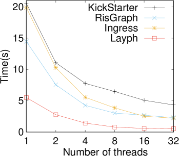
We first compare with the competitors in response time of each workload executed on different datasets. The Normalized results are reported in Figure 5, where the response time of is treated as the baseline, i.e., finishes in unit time 1. In particular, Figure 5e reports the response time for processing vertex updates, while the rest is used for edge updates. We can see that the improvement in handling vertex changes in is consistent with the improvement in handling edge changes. When updating vertices, the other systems meet runtime errors, thus we only compare Ingress with . It is shown that consistently outperforms others in most cases. Specifically, achieves 3.13-15.82 (8.49 on average) speedup over KickStarter, 2.54-8.49 (4.49 on average) speedup over RisGraph, 2.99-36.66 (18.99 on average) speedup over GraphBolt, 2.92-32.93 (17.53 on average) speedup over DZiG, and 1.06-7.22 (2.54 on average) speedup over Ingress. To explain the reason for the above results, we also report the total number of edge activations in Figure 6. An edge activation represents an operation. In most graph workloads, the cost of is much greater than that of operation, because the number of and the unit cost of are often both larger than that of . From Figure 5 and Figure 6, we can see that the normalized number of edge activations is a similar trend to the normalized response time of each system.
Regarding and , RisGraph is faster than KickStarter since it allows more parallelism during incremental updates and allows for localized data access. Ingress and RisGraph are comparable because the memoization-path engine in Ingress follows a similar idea. outperforms the other competitors by leveraging the layered graph. Note that, when performing BFS on WB, RigGraph is slower than but with fewer edge activations. This is because that RisGraph can identify the safe and unsafe updates to reduce edge activations. It just so happens that most of the updates on WB are safe for . However, the additional cost of identifying the safe or unsafe is relatively expensive since WB is very small. While in SSSP, compared with Ingress, also requires less response time but with more edge activations. This is because there are some large dense subgraphs in WB, requiring more shortcut updates, which increase the number of edge activations. Since is parallel-friendly for shortcut updates, it will only have a small effect on the response time.
Regarding and , DZiG is faster than GraphBolt since DZiG has a sparsity detection mechanism, based on which it can adjust the incremental computation scheme. Besides, Ingress is faster than DZiG and GraphBolt. This can be attributed to its memoization-free engine which is more efficient than others. is built on top of Ingress, and can further limit the iterative computation scope with the layered graph, which reduces the number of activation edges, as shown in Figure 6. We find that exhibits less improvement on WB. The reason is that the subgraphs in WB are much larger than that in other graphs, which increases costs and weakens gains. The reason will be further explained in Section VI-F.
VI-C Runtime Breakdown
During incremental computation, consists of four phases: the layered graph update, revision messages upload, iterative computation on the upper layer, and messages assignment. To study the time spent in each phase, we run four algorithms on UK and record the runtime of each phase. The proportion of runtime for different phases is shown in Figure 8. We can see that the iterative computation takes up most of the runtime. The messages assignment is the second most expensive phase. The layered graph update and revision messages upload are both very fast except in . This is because the iterative computation of is very fast, say 418 ms, which makes those two phases relatively longer. The results indicate that the additional cost in our system, i.e., the maintenance of the layered graph, is lightweight. Based on the above experimental analysis, it is worth adopting the layered graph in incremental graph processing.
VI-D Varying Number of Threads
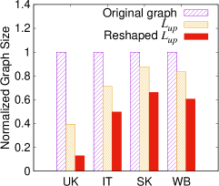
We vary the number of execution threads from 1 to 32 to see the runtime reduction. We run on UK and compare with KickStarter, RisGraph, and Ingress. The results are shown in Figure 9a. We can see that as the threads increase, the runtime decreases steadily in all systems as expected. The reduction is smoother when the number of threads is larger than 8. This is because all these systems use atomic operations to guarantee correctness, hence threads will lead to more write-write conflicts which will hurt parallelism. Compared with the runtime with 1 thread, with 32 threads can achieve 10.1 speedup, which is higher than KickStarter (4.7 speedup), RisGraph (6.2 speedup), and Ingress (9.0 speedup). We also run on UK and compare with GraphBolt, DZiG, and Ingress. The results are reported in Figure 9b where a base-10 log scale is used for the Y axis. We can observe that GraphBolt, DZiG, and show better scaling performance than Ingress. The reason is that the problem of the write-write conflict in is more serious than that in . In GraphBolt and DZiG, vertex states need to be recorded during each iteration, which can alleviate the conflict problem with massive space cost in sacrifice. In , both the shortcut update process and the local assignment process contain many independent local computations, making more parallel-friendly. Therefore, can benefit more from parallelism.
VI-E Varying Amount of Updates
To study the performance with different amounts of updates, we vary the size of the updates set (a.k.a. batch size) from 10 to 10 million on UK and compare with the competitors when running and . Figure 10 shows the speedup results of over the competitors. The speedup is more significant with a smaller batch size because utilizes the layered graph to effectively reduce the scope of global iterations. In , if the batch size is too small, e.g., 10, the effects of these updates might only be applied within subgraphs, thus the iterative computations are constrained in affected subgraphs. However, the speedup is less significant when the batch size gets larger. This is because more updates are likely to affect more subgraphs in our system, which increases the shortcut update cost and undermines the benefits of the layered graph. However, large batches of updates will prolong the response time and lose the real-time property, so smaller batches of updates are preferable for delay-sensitive applications or online applications.
VI-F Effect of Vertex Replication
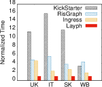
To verify the effectiveness of vertex replication proposed in Section IV-A1, we measure the sizes of the original graphs, the original upper layers, and the reshaped upper layers as shown in Figure 8a. We can see that the sizes of the original graphs are greatly reduced (by 12%-60%) by using the layered graph, and the sizes of the original upper layers are further reduced (by 34%-87%) through vertex replication. We also run and on the original graph with Ingress, the original upper layer with (without vertex replication), and the reshaped upper layer with . The runtime results are reported in Figure 8b and Figure 8c, respectively. We can see that most of the runtime results are proportional to their graph sizes or the upper layer sizes. It is noticeable that the runtime of on WB by is longer with vertex replication than without vertex replication. By digging into the graph property, we find that the sizes of subgraphs in WB are very large. With vertex replication, an edge update could incur multiple local recomputations on multiple subgraphs that are correlated to this updated edge. Therefore, if many large subgraphs are affected, the layered graph update cost for shortcut calculations is evident, which may overweigh the benefits. On the contrary, if the size of the affected subgraph is small, this will not impact performance as the shortcut calculation will be very fast.
VI-G Analysis of Additional Overhead


To evaluate the effect of additional space and offline operations on , we first report the additional space cost of in Figure 11a. We can see that the additional space cost brought by the layered graph is 37.89%, 61.53%, 19.79%, and 0.32% of the original graph, which is acceptable. We then report the offline preprocessing time ( offline), the accumulative incremental computation time of ( acc. inc.), and that of Ingress (Ingress acc. inc.) in Figure 11b when performing SSSP on UK. It is shown that after 9 runs of incremental computation, the runtime of , including the offline time and the accumulative incremental computation time, becomes less than Ingress. This is because the offline operation is performed only once but can bring a significant performance gain on each incremental computation.
VII Related Work
Incremental Graph Processing Systems. Incremental processing for evolving graphs has attracted great attention in recent years [16, 29, 30, 14, 15, 17, 18, 31, 32, 33, 34, 35, 36, 37, 38, 39, 40, 41]. Tornado [29] provides loop-based incrementalization support for the fix-point graph computations. KickStarter [14] maintains a dependency tree to memorize the critical paths for converged states and performs necessary adjustments to accommodate changes. RisGraph [18] deduces safe approximation results upon graph updates and fixes these results via iterative computation. GraphBolt [15] keeps track of the dependencies via the memorized intermediate states among iterations and adjusts the dependencies iteration-by-iteration to achieve incremental computation. i2MapReduce [38, 39] extends Hadoop MapReduce to support incremental iterative graph computations by memorizing the intermediate map/reduce output. Similarly, many other works, e.g., DZiG [17] and HBSP model [41], also memorize and reuse the previous computations to minimize useless re-execution. Ingress [16] can automatically select the best memoization scheme according to algorithm property. The above systems propagate the effects of graph updates over the whole graph, which causes a large number of vertices and edges to be activated, and ultimately leads to a large number of computations.
Hardware Accelerators for Incremental Graph Processing. A number of solutions based on new hardware to accelerate dynamic graph processing have been proposed recently [42, 43, 44, 45, 37]. GraSU [42] provides the first FPGA-based high-throughput graph update library for dynamic graphs. It accelerates graph updates by exploiting spatial similarity. JetStream [43] extends the event-based accelerator [20] for graph workloads to support streaming updates. It works well on both accumulative and monotonic graph algorithms. [44] proposes input-aware software and hardware solutions to improve the performance of incremental graph updates and processing. TDGraph [45] proposes efficient topology-driven incremental execution methods in accelerator design for more regular state propagation and better data locality.
Incremental Graph Algorithms. There are also a number of incremental methods proposed for specific algorithms, e.g., regular path queries [46], strongly connected components [47], subgraph isomorphism [48], k-cores [49], graph partitioning [50, 51] and triangle counting [52]. In contrast to these algorithm-specific methods, our framework extends Ingress [16], which can automatically deduce incremental algorithms from the batch counterparts by a generic approach. It supports a series of incremental graph algorithms with different computation patterns, i.e., traversal-based (e.g., SSSP and BFS) and iteration-based (e.g., PageRank and PHP).
Partition-based Methods. Some partition-based methods have been proposed to improve graph processing, such as Blogel [53], Giraph++ [54], Grace [55], GRAPE [13]. They employ a block-centric (or subgraph-centric) framework to process graphs and try to reduce the communication overhead between threads or processors (reducing the information flow between subgraphs). However, these systems are designed for static graph processing. Different from these existing approaches, the novelty of lies in that we propose a layered graph structure to improve the incremental graph processing for dynamic graphs, which aims to reduce the computation caused by massive message propagation.
VIII Conclusions
We have proposed , a framework to accelerate incremental graph processing by layering graph. It relies on limiting global iterative computations on the original graph to a few independent small-scale local iterative computations on the lower layer, which is used to update shortcuts and upload messages, and a global computation on the upper layer graph skeleton. This greatly fits incremental computation for evolving graphs since the number of vertices and edges involved in iterative computations is effectively limited by our layered graph. Specifically, only the dense subgraphs affected by on the lower layer and the graph skeleton on the upper layer perform iterative computations. is implemented on top of our previous work Ingress to support message-driven incremental computation. Our experimental study verifies that can greatly improve incremental processing performance for dynamic graphs.
Acknowledgment
The work is supported by the National Natural Science Foundation of China (62072082, U2241212, U1811261, 62202088, 62202301), the National Social Science Foundation of China (21&ZD124), the Fundamental Research Funds for the Central Universities (N2216012, N2216015), the Key R&D Program of Liaoning Province (2020JH2/10100037), and a research grant from Alibaba Innovative Research (AIR) Program.
References
- [1] J. Tang, T. Wang, J. Wang, and D. Wei, “Efficient social network approximate analysis on blogosphere based on network structure characteristics,” in Proceedings of the 3rd Workshop on Social Network Mining and Analysis, SNAKDD 2009, Paris, France, June 28, 2009. ACM, 2009, p. 7.
- [2] L. Page, S. Brin, R. Motwani, and T. Winograd, “The pagerank citation ranking: Bringing order to the web.” Stanford InfoLab, Tech. Rep., 1999.
- [3] J. Cho, S. Roy, and R. Adams, “Page quality: In search of an unbiased web ranking,” in Proceedings of the ACM SIGMOD International Conference on Management of Data, Baltimore, Maryland, USA, June 14-16, 2005. ACM, 2005, pp. 551–562.
- [4] Y. Ahn, S. Park, S. Lee, and S. Lee, “A heterogeneous graph-based recommendation simulator,” in Seventh ACM Conference on Recommender Systems, RecSys ’13, Hong Kong, China, October 12-16, 2013. ACM, 2013, pp. 471–472.
- [5] B. Berger, R. Singh, and J. Xu, “Graph algorithms for biological systems analysis,” in Proceedings of the Nineteenth Annual ACM-SIAM Symposium on Discrete Algorithms, SODA 2008, San Francisco, California, USA, January 20-22, 2008. SIAM, 2008, pp. 142–151.
-
[6]
“Size of Wikipedia,” 2020, https://en.wikipedia.org/wiki/Wikipedia:Size
_of_Wikipedia. - [7] G. Malewicz, M. H. Austern, A. J. C. Bik, J. C. Dehnert, I. Horn, N. Leiser, and G. Czajkowski, “Pregel: a system for large-scale graph processing,” in Proceedings of the ACM SIGMOD International Conference on Management of Data, SIGMOD 2010, Indianapolis, Indiana, USA, June 6-10, 2010. ACM, 2010, pp. 135–146.
- [8] J. E. Gonzalez, Y. Low, H. Gu, D. Bickson, and C. Guestrin, “Powergraph: Distributed graph-parallel computation on natural graphs,” in 10th USENIX Symposium on Operating Systems Design and Implementation, OSDI 2012, Hollywood, CA, USA, October 8-10, 2012. USENIX Association, 2012, pp. 17–30.
- [9] Q. Wang, Y. Zhang, H. Wang, L. Geng, R. Lee, X. Zhang, and G. Yu, “Automating incremental and asynchronous evaluation for recursive aggregate data processing,” in Proceedings of the 2020 International Conference on Management of Data, SIGMOD Conference 2020, online conference [Portland, OR, USA], June 14-19, 2020. ACM, 2020, pp. 2439–2454.
- [10] Y. Zhang, Q. Gao, L. Gao, and C. Wang, “Maiter: An asynchronous graph processing framework for delta-based accumulative iterative computation,” IEEE Trans. Parallel Distributed Syst., vol. 25, no. 8, pp. 2091–2100, 2014.
- [11] Z. Yanfeng, G. Qixin, G. Lixin, and W. Cuirong, “Priter: a distributed framework for prioritized iterative computations,” in ACM Symposium on Cloud Computing in conjunction with SOSP 2011, SOCC ’11, Cascais, Portugal, October 26-28, 2011. ACM, 2011, p. 13.
- [12] X. Zhu, W. Chen, W. Zheng, and X. Ma, “Gemini: A computation-centric distributed graph processing system,” in 12th USENIX Symposium on Operating Systems Design and Implementation, OSDI 2016, Savannah, GA, USA, November 2-4, 2016. USENIX Association, 2016, pp. 301–316.
- [13] W. Fan, J. Xu, Y. Wu, W. Yu, J. Jiang, Z. Zheng, B. Zhang, Y. Cao, and C. Tian, “Parallelizing sequential graph computations,” in Proceedings of the 2017 ACM International Conference on Management of Data, SIGMOD Conference 2017, Chicago, IL, USA, May 14-19, 2017. ACM, 2017, pp. 495–510.
- [14] K. Vora, R. Gupta, and G. Xu, “Kickstarter: Fast and accurate computations on streaming graphs via trimmed approximations,” in Proceedings of the Twenty-Second International Conference on Architectural Support for Programming Languages and Operating Systems, ASPLOS 2017, Xi’an, China, April 8-12, 2017. ACM, 2017, pp. 237–251.
- [15] M. Mariappan and K. Vora, “Graphbolt: Dependency-driven synchronous processing of streaming graphs,” in Proceedings of the Fourteenth EuroSys Conference 2019, Dresden, Germany, March 25-28, 2019. ACM, 2019, pp. 25:1–25:16.
- [16] S. Gong, C. Tian, Q. Yin, W. Yu, Y. Zhang, L. Geng, S. Yu, G. Yu, and J. Zhou, “Automating incremental graph processing with flexible memoization,” Proc. VLDB Endow., vol. 14, no. 9, pp. 1613–1625, 2021.
- [17] M. Mariappan, J. Che, and K. Vora, “Dzig: sparsity-aware incremental processing of streaming graphs,” in EuroSys ’21: Sixteenth European Conference on Computer Systems, Online Event, United Kingdom, April 26-28, 2021. ACM, 2021, pp. 83–98.
- [18] G. Feng, Z. Ma, D. Li, S. Chen, X. Zhu, W. Han, and W. Chen, “Risgraph: A real-time streaming system for evolving graphs to support sub-millisecond per-update analysis at millions ops/s,” in SIGMOD ’21: International Conference on Management of Data, Virtual Event, China, June 20-25, 2021. ACM, 2021, pp. 513–527.
- [19] “libgrape-lite,” 2020, https://github.com/alibaba/libgrape-lite.
- [20] S. Rahman, N. B. Abu-Ghazaleh, and R. Gupta, “Graphpulse: An event-driven hardware accelerator for asynchronous graph processing,” in 53rd Annual IEEE/ACM International Symposium on Microarchitecture, MICRO 2020, Athens, Greece, October 17-21, 2020. IEEE, 2020, pp. 908–921.
- [21] V. D. Blondel, J.-L. Guillaume, R. Lambiotte, and E. Lefebvre, “Fast unfolding of communities in large networks,” Journal of statistical mechanics: theory and experiment, vol. 2008, no. 10, p. P10008, 2008.
- [22] D. Zhuang, J. M. Chang, and M. Li, “Dynamo: Dynamic community detection by incrementally maximizing modularity,” IEEE Trans. Knowl. Data Eng., vol. 33, no. 5, pp. 1934–1945, 2021.
- [23] M. Seifikar, S. Farzi, and M. Barati, “C-blondel: An efficient louvain-based dynamic community detection algorithm,” IEEE Trans. Comput. Soc. Syst., vol. 7, no. 2, pp. 308–318, 2020.
-
[24]
“uk-2005,” 2005, https://www.cise.ufl.edu/research/sparse/matrices/LAW
/uk-2005.html. - [25] “it-2004,” https://law.di.unimi.it/webdata/it-2004/, 2004.
- [26] “sk-2005,” https://law.di.unimi.it/webdata/sk-2005/, 2005.
- [27] R. A. Rossi and N. K. Ahmed, “The network data repository with interactive graph analytics and visualization,” in Proceedings of the Twenty-Ninth AAAI Conference on Artificial Intelligence, January 25-30, 2015, Austin, Texas, USA. AAAI Press, 2015, pp. 4292–4293.
- [28] Z. Guan, J. Wu, Q. Zhang, A. K. Singh, and X. Yan, “Assessing and ranking structural correlations in graphs,” in Proceedings of the ACM SIGMOD International Conference on Management of Data, SIGMOD 2011, Athens, Greece, June 12-16, 2011. ACM, 2011, pp. 937–948.
- [29] X. Shi, B. Cui, Y. Shao, and Y. Tong, “Tornado: A system for real-time iterative analysis over evolving data,” in Proceedings of the 2016 International Conference on Management of Data, SIGMOD Conference 2016, San Francisco, CA, USA, June 26 - July 01, 2016. ACM, 2016, pp. 417–430.
- [30] D. Sengupta, N. Sundaram, X. Zhu, T. L. Willke, J. S. Young, M. Wolf, and K. Schwan, “Graphin: An online high performance incremental graph processing framework,” in Euro-Par 2016: Parallel Processing - 22nd International Conference on Parallel and Distributed Computing, Grenoble, France, August 24-26, 2016, Proceedings, ser. Lecture Notes in Computer Science, vol. 9833. Springer, 2016, pp. 319–333.
- [31] S. Ko, T. Lee, K. Hong, W. Lee, I. Seo, J. Seo, and W. Han, “iturbograph: Scaling and automating incremental graph analytics,” in SIGMOD ’21: International Conference on Management of Data, Virtual Event, China, June 20-25, 2021. ACM, 2021, pp. 977–990.
- [32] X. Jiang, C. Xu, X. Yin, Z. Zhao, and R. Gupta, “Tripoline: generalized incremental graph processing via graph triangle inequality,” in EuroSys ’21: Sixteenth European Conference on Computer Systems, Online Event, United Kingdom, April 26-28, 2021. ACM, 2021, pp. 17–32.
- [33] T. A. K. Zakian, L. A. R. Capelli, and Z. Hu, “Incrementalization of vertex-centric programs,” in 2019 IEEE International Parallel and Distributed Processing Symposium, IPDPS 2019, Rio de Janeiro, Brazil, May 20-24, 2019. IEEE, 2019, pp. 1019–1029.
- [34] D. G. Murray, F. McSherry, R. Isaacs, M. Isard, P. Barham, and M. Abadi, “Naiad: a timely dataflow system,” in ACM SIGOPS 24th Symposium on Operating Systems Principles, SOSP ’13, Farmington, PA, USA, November 3-6, 2013. ACM, 2013, pp. 439–455.
- [35] F. McSherry, D. G. Murray, R. Isaacs, and M. Isard, “Differential dataflow,” in Sixth Biennial Conference on Innovative Data Systems Research, CIDR 2013, Asilomar, CA, USA, January 6-9, 2013, Online Proceedings. www.cidrdb.org, 2013.
- [36] P. Vaziri and K. Vora, “Controlling memory footprint of stateful streaming graph processing,” in 2021 USENIX Annual Technical Conference, USENIX ATC 2021, July 14-16, 2021, I. Calciu and G. Kuenning, Eds. USENIX Association, 2021, pp. 269–283.
- [37] D. Chen, C. Gui, Y. Zhang, H. Jin, L. Zheng, Y. Huang, and X. Liao, “Graphfly: efficient asynchronous streaming graphs processing via dependency-flow,” in 2022 SC22: International Conference for High Performance Computing, Networking, Storage and Analysis (SC), 2022, pp. 632–645.
- [38] Y. Zhang, S. Chen, Q. Wang, and G. Yu, “i2mapreduce: Incremental mapreduce for mining evolving big data,” in 32nd IEEE International Conference on Data Engineering, ICDE 2016, Helsinki, Finland, May 16-20, 2016. IEEE Computer Society, 2016, pp. 1482–1483.
- [39] Y. Zhang and S. Chen, “imapreduce: incremental iterative mapreduce,” in 2nd International Workshop on Cloud Intelligence (colocated with VLDB 2013), Cloud-I ’13, Riva del Garda, Trento, Italy, August 26, 2013. ACM, 2013, pp. 3:1–3:4.
- [40] Z. Cai, D. Logothetis, and G. Siganos, “Facilitating real-time graph mining,” in Proceedings of the Fourth International Workshop on Cloud Data Management, CloudDB 2012, Maui, HI, USA, October 29, 2012. ACM, 2012, pp. 1–8.
- [41] C. Wickramaarachchi, C. Chelmis, and V. K. Prasanna, “Empowering fast incremental computation over large scale dynamic graphs,” in 2015 IEEE International Parallel and Distributed Processing Symposium Workshop, IPDPS 2015, Hyderabad, India, May 25-29, 2015. IEEE Computer Society, 2015, pp. 1166–1171.
- [42] Q. Wang, L. Zheng, Y. Huang, P. Yao, C. Gui, X. Liao, H. Jin, W. Jiang, and F. Mao, “Grasu: A fast graph update library for fpga-based dynamic graph processing,” in FPGA ’21: The 2021 ACM/SIGDA International Symposium on Field Programmable Gate Arrays, Virtual Event, USA, February 28 - March 2, 2021. ACM, 2021, pp. 149–159.
- [43] S. Rahman, M. Afarin, N. B. Abu-Ghazaleh, and R. Gupta, “Jetstream: Graph analytics on streaming data with event-driven hardware accelerator,” in MICRO ’21: 54th Annual IEEE/ACM International Symposium on Microarchitecture, Virtual Event, Greece, October 18-22, 2021. ACM, 2021, pp. 1091–1105.
- [44] A. Basak, Z. Qu, J. Lin, A. R. Alameldeen, Z. Chishti, Y. Ding, and Y. Xie, “Improving streaming graph processing performance using input knowledge,” in MICRO ’21: 54th Annual IEEE/ACM International Symposium on Microarchitecture, Virtual Event, Greece, October 18-22, 2021. ACM, 2021, pp. 1036–1050.
- [45] J. Zhao, Y. Yang, Y. Zhang, X. Liao, L. Gu, L. He, B. He, H. Jin, H. Liu, X. Jiang, and H. Yu, “Tdgraph: a topology-driven accelerator for high-performance streaming graph processing,” in ISCA ’22: The 49th Annual International Symposium on Computer Architecture, New York, New York, USA, June 18 - 22, 2022. ACM, 2022, pp. 116–129.
- [46] W. Fan, C. Hu, and C. Tian, “Incremental graph computations: Doable and undoable,” in Proceedings of the 2017 ACM International Conference on Management of Data, SIGMOD Conference 2017, Chicago, IL, USA, May 14-19, 2017. ACM, 2017, pp. 155–169.
- [47] J. Holm, K. de Lichtenberg, and M. Thorup, “Poly-logarithmic deterministic fully-dynamic algorithms for connectivity, minimum spanning tree, 2-edge, and biconnectivity,” Journal of the ACM, vol. 48, no. 4, pp. 723–760, 2001.
- [48] K. Kim, I. Seo, W. Han, J. Lee, S. Hong, H. Chafi, H. Shin, and G. Jeong, “Turboflux: A fast continuous subgraph matching system for streaming graph data,” in Proceedings of the 2018 International Conference on Management of Data, SIGMOD Conference 2018, Houston, TX, USA, June 10-15, 2018. ACM, 2018, pp. 411–426.
- [49] R. Li, J. X. Yu, and R. Mao, “Efficient core maintenance in large dynamic graphs,” IEEE Trans. Knowl. Data Eng., vol. 26, no. 10, pp. 2453–2465, 2014.
- [50] W. Fan, M. Liu, C. Tian, R. Xu, and J. Zhou, “Incrementalization of graph partitioning algorithms,” Proc. VLDB Endow., vol. 13, no. 8, pp. 1261–1274, 2020.
- [51] W. Fan, C. Hu, M. Liu, P. Lu, Q. Yin, and J. Zhou, “Dynamic scaling for parallel graph computations,” Proc. VLDB Endow., vol. 12, no. 8, pp. 877–890, 2019.
- [52] A. McGregor, S. Vorotnikova, and H. T. Vu, “Better algorithms for counting triangles in data streams,” in Proceedings of the 35th ACM SIGMOD-SIGACT-SIGAI Symposium on Principles of Database Systems, PODS 2016, San Francisco, CA, USA, June 26 - July 01, 2016. ACM, 2016, pp. 401–411.
- [53] D. Yan, J. Cheng, Y. Lu, and W. Ng, “Blogel: A block-centric framework for distributed computation on real-world graphs,” Proc. VLDB Endow., vol. 7, no. 14, pp. 1981–1992, 2014.
- [54] Y. Tian, A. Balmin, S. A. Corsten, S. Tatikonda, and J. McPherson, “From ”think like a vertex” to ”think like a graph”,” Proc. VLDB Endow., vol. 7, no. 3, pp. 193–204, 2013.
- [55] W. Xie, G. Wang, D. Bindel, A. J. Demers, and J. Gehrke, “Fast iterative graph computation with block updates,” Proc. VLDB Endow., vol. 6, no. 14, pp. 2014–2025, 2013.