Lattice QCD study of color correlations between static quarks with gluonic excitations
Abstract
We study the color correlation between static quark and antiquark () that is accompanied by gluonic excitations in the confined phase at by constructing reduced density matrices in color space. We perform quenched lattice QCD calculations with the Coulomb gauge adopting the standard Wilson gauge action, and the spatial volume is at , which corresponds to the lattice spacing fm and the system volume fm3. We evaluate the color density matrix of static pairs in 6 channels (, , , , , ), and investigate the interquark-distance dependence of color correlations. We find that as the interquark distance increases, the color correlation quenches because of color leak into the gluon field and finally approaches the random color configuration in the systems with and without gluonic excitations. For this color screening effect, we evaluate the ”screening mass” to discuss its dependence on channels, the quantum number of the gluonic excitations.
I Introduction
Color confinement is one of the most prominent features of Quantum ChromoDynamics (QCD), and is still attracting great interest. QCD in the confined phase gives a linearly rising potential between static quarks, and confines quarks within a totally color-singlet hadron. Such confining features have been studied and confirmed in a variety of approaches [1]. The color confinement can be explained by a gluonic flux tube that is nonperturbatively formed among quarks. A color flux tube with a constant energy per length is formed between a quark and an antiquark in the color singlet channel, and this one-dimensional tube leads to the linearly rising quark and antiquark () potential [2, 3].
The in-between flux tube is a colored gluonic object created by end-point color sources, quarks. The color charge initially associated with a color-singlet pair flows into interquark region, and forms a flux tube as the interquark distance is enlarged keeping the total system color singlet [4, 5]. This color transfer from quarks to the flux tube can be regarded as a color charge leak from quarks to the gluon fields, and is quantified as the color screening effect among quarks. When interquark distance is small at , color leak into gluon fields (flux tube) hardly occurs and the quarks’ color correlation is maximal. As the interquark distance gets larger, the gluonic flux tube is formed and quarks’ color is screened by it, which reduces the quarks’ color correlation. This correlation quench is expressed as a mixture of a “random” color configuration, in which color singlet and octet components equally contribute. Finally at , the correlation disappears and the quarks’ color configuration is expressed solely by a random color configuration [6].
In Refs. [6, 7], the color correlation between static quark and antiquark was investigated, and the dependence of the color correlation for and systems was clarified in detail by analyzing the reduced density matrix . In the series of papers, we also investigated entanglement entropy (EE) computed from . The EE under the presence of flux tube has been recently investigated in a gauge-invariant manner [8], and such analyses are expected to lead to further clarification of the nonperturbative aspects of QCD.
A gluonic excitation of gluon fields is also an intriguing issue and has been studied in many situations [9, 10, 11]. A quark and antiquark () potential with gluonic excitations (hybrid potential) was intensively studied and precisely determined, for instance, in Ref. [9]. A system with gluonic excitations might be understood as a bound state of a color octet pair and constituent gluons [12, 13, 14, 15, 16, 17, 18]. In this picture, quark and antiquark are expected to form a color octet configuration at , which couples with a constituent gluon to be totally a color singlet state. This is in contrast to the ground-state system without gluonic excitations, where quarks form a color singlet configuration at . Hadrons accompanied by gluonic excitations are also called hybrid hadrons, and clarification of the internal color structure of such systems will lead to a deeper understanding of matters obeying the strong interaction.
In this paper, we define the reduced density matrix for a static pair with gluonic excitations in terms of color degrees of freedom. According to the ansatz for the reduced density matrix proposed in Ref. [6], we investigate the color correlation inside a pair and determine the dependence of the correlation. In Sec. II, we give the formalism to compute the reduced density matrix of a system. The details of numerical calculations and ansatz for are also shown in Sec. II. Results are presented in Sec. III. Sec. IV is devoted to the summary and concluding remarks.
II Formalism
II.1 reduced 2-body density matrix and correlation
We investigate the color correlation between static quark and antiquark () by the two-body density matrix evaluated in terms of ’s color configuration. A density matrix defined in such a way is nothing but the reduced density matrix that is obtained integrating out the other DOF (e.g. gluonic DOF) in the full density matrix. A reduced two-body density operator for a system with the interquark distance is defined as
| (1) |
Here represents a quantum state in which the antiquark is located at the origin and the other quark lies at . The matrix elements of the reduced density operator, where and ( and ) are quark’s (antiquark’s) color indices, are expressed as
| (2) |
Then, is an square matrix with the dimension . The density matrix is evaluated using only quark’s color DOF, but does not explicitly contain gluon’s color DOF in this construction: the gluonic DOF are “integrated out” in the lattice calculation, and can be regarded as a reduced density matrix.
II.2 Ansatz for reduced density matrix
For the time being, we consider a quark and antiquark system without gluonic excitations. In previous studies [6, 7], we found that the reduced color density matrix evaluated by lattice QCD can be precisely reproduced with an ansatz, where is expressed as a sum of an “initial” color singlet configuration at and mixing of the random color configuration due to the color screening effect between quark and antiquark at finite .
Let the density operator for quark and antiquark forming a color singlet state in the Coulomb gauge as
| (3) |
In color SU() QCD, the density operator for a pair in an adjoint state is expressed as
| (4) |
In the limit of , quark and antiquark are considered to form a color-singlet state () corresponding to the strong correlation limit, since there exists no gluonic excitation in the system and gluons form a totally colorless state. Its density operator will be written as
| (5) |
Here, the subscript “” means that the matrix is expressed in terms of ’s color representation with the vector set of .
As increases, an uncorrelated state represented by random color configurations, where all the components mix with equal weights, enters in due to the color screening effect by in-between gluons. The density operator for such a random-color state is given as
| (6) | |||||
Letting the fraction of the initial color singlet state being and that of the random contribution being , the density operator for an interquark distance of in this ansatz is written as
| (7) |
Here, the subscript means that the density operator is dominated by the color singlet contribution at . can be explicitly expressed as
| (8) | |||||
| (9) | |||||
| (10) | |||||
| (11) |
In this ansatz,
| (12) |
are satisfied at any . The normalization condition is trivially satisfied in this ansatz as
| (13) |
where . It was found that this ansatz reproduces the density matrix element for the ground-state system ( channel) evaluated by lattice QCD calculation with a very good accuracy.
This ansatz can be extended to the system with gluonic excitations. In what follows, we limit ourselves to case, hence we refer to “adjoint” states as “octet” ones. In a system accompanied by gluonic excitations, a pair can also form a color octet configuration at region, where excited gluons carry octet color and the total system is kept color singlet. With the density operator averaged for octet states
| (14) |
the ansatz for a system with gluonic excitations takes the form
| (15) | |||||
| (16) | |||||
| (17) |
Here, represents the fraction of the initial color octet state, and the subscript means that the density operator is dominated by the color octet contribution at .
In the later sections, we see that this ansatz actually reproduces the color density matrix for a static system with gluonic excitations.
II.3 Lattice QCD formalism
In a static system, there exist three quantum numbers. One is the eigenvalue of the projected total angular momentum , where is the total angular momentum gluon fields possess and is the unit vector parallel to the axis. We assign capital Greek letters ,.. for states. Second is the eigenvalue of the simultaneous operations of charge conjugation and spatial inversion about the midpoint between . States with are denoted by the subscripts . Third is a label adopted only for the channel. Even (odd) states under the reflection in a plane that contains the axis are represented by the superscripts . The first excited state in each channel is discriminated by a prime mark. Then, the quantum numbers for each state investigated in this paper are denoted as
The position on the lattice site is denoted as , and the -direction () link variable at is expressed as . With a lower staple representing pair creation and propagation and an upper staple for pair annihilation that are defined as
| (18) |
| (19) |
we compute as
| (20) |
Here, -state creation/annihilation operator that connects and sites at is constructed so that it creates a state with a quantum number [9, 10]. For example, when , we simply adopt
| (21) |
The superscripts denote the smearing levels for spatial link variables. We finally construct the operator which encodes the elements of the density matrix for -th excited state in the channel as
| (22) |
where the coefficients are determined so as to maximize the overlap of the creation/annihilation operator to -th excited state signals. The operator optimization is done by solving a generalized eigenvalue problem [19, 20, 11] for potentials in the target channel . When couples only to the -th excited state in the channel, is then expressed as
| (23) | |||||
where is the -th excited-state energy. Normalizing so that , we finally obtain the two-body color density matrix for the -th excited state in the channel whose trace is unity ().
II.4 Lattice QCD parameters
We performed quenched calculations for reduced density matrices of static quark and antiquark () systems adopting the standard Wilson gauge action. The gauge configurations are generated on the spatial volume of with the gauge couplings , which corresponds to [fm3]. The temporal extent is . All the gauge configurations are gauge-fixed with the Coulomb gauge condition. While finite volume effects would still remains for [fm3] [6], detailed study taking care of such systematic errors is beyond the scope of the present paper, in which the color structure of a pair with gluonic excitations is clarified for the first time.
III Lattice QCD results
III.1 Energy spectrum
In Fig. 1, the energy spectra for , , , , and are plotted as a function of interquark distance . The state with the lowest excitation is the state, and and states are the second-lowest excited states that almost degenerate in energy. The state’s energy is higher than theirs. These spectra can be compared with the data of the preceding lattice QCD calculation [9] and the data obtained in this study are found to be consistent with them within errors. The energy for channel, which was not computed in Ref. [9], lies above that for channel.

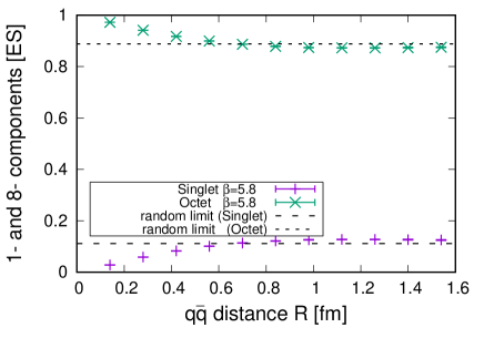
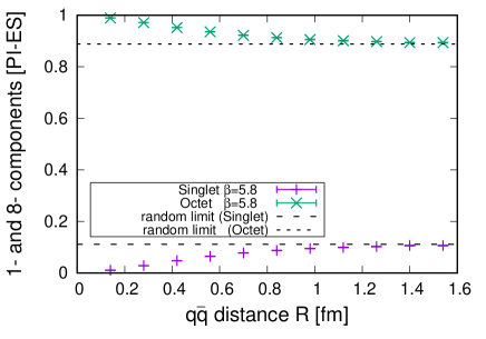
III.2 Singlet and octet components
Figure 2 shows the dependence of the singlet and octet components and for the channel, and Figs. 3-7 demonstrate those for the excited channels, , , , and , respectively. One can find that a pair in the channel forms a purely color singlet configuration at , and the ratio approaches of the random color configuration as increases. The dependence is consistent with the previous work [6], and we confirm that the diagonalization process of the Hamiltonian is successful. This result indicates that in-between flux-tube formation is expressed by the color leak from color sources to a flux tube, which can be quantified as the color screening effect among color sources, quarks. It is of great interest that pairs in all the gluonically excited channels form a purely color octet configuration at . It is consistent with a simple gluonic excitation picture, where a pair and one constituent gluon are bound. The random color configuration is mixed as increases, and in the limit of , the ratio of and again approaches that for the random color configuration, . This observation supports the scenario that the color screening effect by the in-between flux tube occurs also in the excited systems.

As shown in the results of and for channel, the speed at which the color configuration approaches the random limit in this channel is the slowest in all the channels, meaning that the singlet correlation remains to some extent. More quantitative discussion of the quenching speed is given in the next subsection.
For the lowest excitation channel, , the color components at small regions are dominated by the octet components, which means that a pair forms a color octet configuration at (See Fig. 4). It is consistent with the constituent gluon picture for gluonic excitation states, where a color octet pair and a color octet constituent gluon are bound to form a totally color singlet physical state. At the large regions, a random color configuration is mixed like channel and the ratio of singlet and octet components again approaches . It means that even in the channels with gluonic excitations, the flux-tube formation emerges as the mixture of random color configurations.
The color components for , , , channels shown in Figs. 3,5,6,7 indicate that these states are also considered to be gluonic excitation states, since the color configurations of them are dominated by a color octet configuration at small . Similarly to the case of the channel, a random color configuration is gradually mixed as increases, and the ratio of singlet and octet components finally approaches . The quenching speed of the color correlation in the , , , channels is faster compared with that in the and channels. A closer look reveals a tiny -independent contribution in the channel: the ratio of singlet and octet components slightly deviates from at the large regions, which is clarified in detail in the later sections.


III.3 dependence of
It is naively expected that a pair in (ground state) channel forms a color singlet configuration at [6, 7], whereas those for other channels (, , , , ) are expected to form an octet color configuration at , since excited gluon fields carry adjoint colors. These behaviors can be confirmed in Figs. 2-7. Then we expect that the ansatz works for channel, and is reasonable for , , , , and channels (See Eqs. (8)(17)) .
We extract and for each channel from the components, and , evaluated with lattice QCD calculations. For example, for , , , , and , we can compute as
| (24) |
Due to the normalization condition
| (25) |
the independent quantity at a given is only or .
We define the fraction of the initial state remaining at for channel as
| (26) |
for , and as
| (27) |
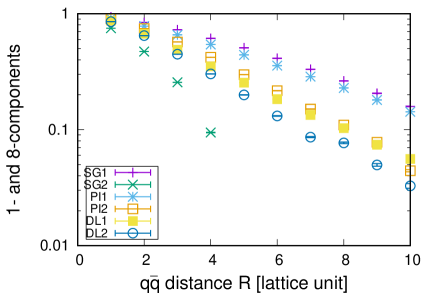
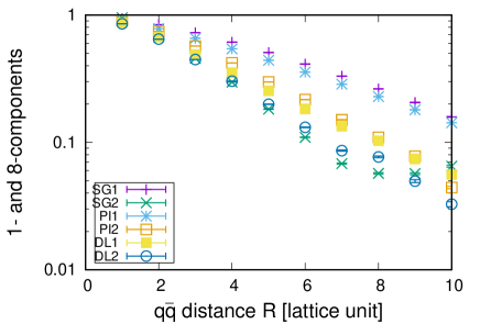
for other channels, , , , , and . In the case of , the initial () color configuration is dominated by a color singlet one, as , hence we adopt instead of . Thus defined indicates the component of the color correlation; it starts from 1 at and decreases as enlarges. calculated for all the channels are logarithmically plotted as a function of the interquark distance in Fig. 8. Most of them show a linear dependence on , which means that initial color correlations are exponentially quenched as increases, and their color configurations approach the random state: can be expressed as . However, the log plot of does not show a clear linear dependence at all regions, and it takes a smaller value than others at small regions. This tendency peculiar to channel implies a negative constant contribution mixed to . Octet components for and ( and ) are compared in Fig. 9.

clearly starts from a smaller value than at small regions, and seems to approach some constant value slightly smaller than , which implies that a negative -independent contribution exists in : is expressed as . A numerical fit gives a offset value , and plotted along with other ’s is shown in Fig. 10.
After this correction, the log plot of shows a clear linear dependence at fm. On the other hand, again goes up at fm . Taking into account that color configurations evaluated presently are strongly affected by a finite volume effect, it might be a finite-volume artifact. In fact, in Fig.11 in Ref. [6], one can find considerable finite-volume effect for fm. Such artifacts can be also found in the fitted parameters (Fig.7 in Ref. [6]). The detailed clarification of color correlation at region with a huge lattice volume is left for future studies.
The exponential decay of the correlation indicates the exponential color screening effects due to in-between gluons. One can find roughly three different magnitudes of slope in Fig. 10. The correlation quenching speed for and channels is the slowest and the color correlation remains at larger . The quenching speed for and channels is faster than that for and channels. Further fast quenching of the color correlation is found in and channels. In the ground state channel , the color leak from quarks to a flux tube is most suppressed. The fact that the color screening speed for the lowest excited channel is comparable with channel in magnitude may indicate that the state has the simplest gluonic excitation mode that does not accelerate the color screening effect. Other excited states are considered to have more complicated gluonic excitation and the color correlation between quarks are easily randomized.
We fit with an exponential function as
| (28) |
and extract the “screening mass” . For the channel, the values of after the correction are used for fitting. The fit range is set to in lattice unit, in which the data show an exponential damping, as seen in Fig. 10.

| 0.200(5) | 0.489(21) | 0.211(2) | 0.338(5) | 0.322(2) | 0.418(1) |
One can categorize the screening masses as,
| (29) |
The screening mass for channel is as small as that for , whereas those for other channels are significantly larger. It might imply that in the viewpoint of color screening effects, the gluonic excitations except for consist of a sum of “fundamental excitations” of the channel.
III.4 Comparison with results at
In Ref. [7], the color structures of a pair at finite temperature were investigated in detail by analyzing the color density matrix as well as the corresponding entanglement entropy, and the color correlations were found to be quickly quenched across the deconfinement phase transition temperature . It means the color configuration is strongly randomized above as the in-between flux tube disappears. Even below , it was found that the color correlation gradually weaken as the temperature rises due to the temperature effect. We here clarify if the temperature effect at can be explained as a thermal ensemble based on the present results for excited states at . We reconstruct the at from the ’s for low-lying 6 channels (, , , , , ), and compare it with the lattice QCD results shown in Ref. [7]. We define the density operator at finite temperature as
| (30) |
where is the temperature of the system and is a energy of a ground-state pair (). In Fig. 12, we show the reconstructed using Eq.(30) as well as the ’s shown in Ref. [7]. Here, the temperature in Eq.(30) is chosen to be 250 MeV.

reconstructed using Eq.(30) is shown by open squares, and filled squares denote at . Other symbols represent ’s at each temperature demonstrated in Ref. [7]. As is seen in Fig. 12, the lattice QCD data at are reproduced by Eq.(30) more or less in the range of fm. Though the coincidence is lost at larger , this deviation is considered to arise from the finite volume effects. The lattice adopted in Ref. [7] is smaller () and the finite volume artifact would remain for large .
IV Summary and concluding remarks
We have investigated the color correlation inside a static quark and antiquark pair accompanied by gluonic excitations (hybrid system) in the confined phase by means of lattice QCD. We have performed quenched lattice QCD calculations with the Coulomb gauge adopting the standard Wilson gauge action, and the spatial volume considered here is at , which corresponds to the lattice spacing fm and the system volume fm3. The reduced density matrix in the color space for a system with the interquark distance has been constructed from link variables and has been analyzed based on the ansatz we proposed in our previous paper. The color density matrix of static pairs have been computed in 6 channels (, , , , , channels), and we have investigated the dependence of color correlations.
For the channel, the ground state channel of a static system, we have confirmed that when is small a pair forms a purely color singlet configuration, which is consistent with our previous study. In the case of hybrid systems with gluonic excitations (, , , , channels), a pair at always forms a purely color octet configuration. This finding is consistent with the constituent gluon picture, where gluonic excitations are expressed by constituent gluons that couple to a static pair.
In all the cases investigated here, as increases, an uncorrelated state represented by random color configurations, where all the components mix with equal weights, enters in due to the color-correlation quenching by in-between gluons, and the ratio of singlet and octet components in finally approaches .
In order to clarify the quenching speed in a quantitative way, we have defined and evaluated the ”screening mass” from the slope of exponential damping of the color correlation. The screening masses for 6 channels satisfy
The screening mass for channel is as small as that for , whereas those for other channels are significantly larger. It might imply that the gluonic excitations except for consist of a sum of “fundamental excitations” of the channel in the viewpoint of color screening effects. In the ground-state channel , the color leak from quarks to a flux tube is most suppressed, and the fact that the color screening speed for the lowest excited channel is the same in magnitude as channel may indicate that the state has the simplest gluonic excitation mode that does not accelerate the color screening effect. Other excited states are considered to have more complicated gluonic excitation and the color correlation between quarks are easily randomized as increases. It would be interesting to clarify the possible relationship between the screening mass and the gluelump mass [21, 22, 17, 23].
We have also tried to reproduce the color density matrix of a pair at finite temperature using the density matirices for low-lying 6 channels at (, , , , , channels), and have found that the lattice QCD data at are reproduced by the thermal average in the range of fm. Note that the color structure of a system in hot medium has been also discussed in different literatures [24, 25, 26].
A future direction for this work would be the analysis of multiquark systems. Multiquark systems are attracting much attention, and clarification of their internal structures has been of great importance. Our method can be easily extended to the analysis of multiquark systems, which is now in progress.
Acknowledgements.
This work was partly supported by Grants-in-Aid of the Japan Society for the Promotion of Science (Grant Nos. 18H05407, 22K03608, 22K03633).References
- [1] J. Greensite, “An Introduction to the Confinement Problem,” Lecture Notes in Physics (Springer, 2011) doi:10.1007/978-3-642-14382-3, and references therein.
- [2] G. S. Bali, K. Schilling and C. Schlichter, Phys. Rev. D 51, 5165 (1995) doi:10.1103/PhysRevD.51.5165 [hep-lat/9409005].
- [3] V. G. Bornyakov et al. [DIK Collaboration], Phys. Rev. D 70, 054506 (2004) doi:10.1103/PhysRevD.70.054506 [hep-lat/0401026].
- [4] G. Tiktopoulos, Phys. Lett. 66B, 271 (1977). doi:10.1016/0370-2693(77)90878-4
- [5] J. Greensite and C. B. Thorn, JHEP 0202, 014 (2002) doi:10.1088/1126-6708/2002/02/014 [hep-ph/0112326].
- [6] T. T. Takahashi and Y. Kanada-En’yo, Phys. Rev. D 100, no.11, 114502 (2019) doi:10.1103/PhysRevD.100.114502 [arXiv:1910.00859 [hep-lat]].
- [7] T. T. Takahashi and Y. Kanada-En’yo, Phys. Rev. D 103, no.3, 034504 (2021) doi:10.1103/PhysRevD.103.034504 [arXiv:2011.10950 [hep-lat]].
- [8] R. Amorosso, S. Syritsyn and R. Venugopalan, [arXiv:2410.00112 [hep-lat]].
- [9] K. J. Juge, J. Kuti and C. Morningstar, Phys. Rev. Lett. 90, 161601 (2003) doi:10.1103/PhysRevLett.90.161601 [arXiv:hep-lat/0207004 [hep-lat]].
- [10] L. Müller, O. Philipsen, C. Reisinger and M. Wagner, Phys. Rev. D 100, no.5, 054503 (2019) doi:10.1103/PhysRevD.100.054503 [arXiv:1907.01482 [hep-lat]].
- [11] P. Bicudo, N. Cardoso and A. Sharifian, Phys. Rev. D 104, no.5, 054512 (2021) doi:10.1103/PhysRevD.104.054512 [arXiv:2105.12159 [hep-lat]].
- [12] D. Horn and J. Mandula, Phys. Rev. D 17, 898 (1978) doi:10.1103/PhysRevD.17.898
- [13] S. Ishida, H. Sawazaki, M. Oda and K. Yamada, Phys. Rev. D 47, 179-198 (1993) doi:10.1103/PhysRevD.47.179
- [14] W. S. Hou, C. S. Luo and G. G. Wong, Phys. Rev. D 64, 014028 (2001) doi:10.1103/PhysRevD.64.014028 [arXiv:hep-ph/0101146 [hep-ph]].
- [15] F. Giacosa, T. Gutsche and A. Faessler, Phys. Rev. C 71, 025202 (2005) doi:10.1103/PhysRevC.71.025202 [arXiv:hep-ph/0408085 [hep-ph]].
- [16] N. Boulanger, F. Buisseret, V. Mathieu and C. Semay, Eur. Phys. J. A 38, 317-330 (2008) doi:10.1140/epja/i2008-10675-5 [arXiv:0806.3174 [hep-ph]].
- [17] M. Berwein, N. Brambilla, J. Tarrús Castellà and A. Vairo, Phys. Rev. D 92, no.11, 114019 (2015) doi:10.1103/PhysRevD.92.114019 [arXiv:1510.04299 [hep-ph]].
- [18] C. Farina, H. Garcia Tecocoatzi, A. Giachino, E. Santopinto and E. S. Swanson, Phys. Rev. D 102, no.1, 014023 (2020) doi:10.1103/PhysRevD.102.014023 [arXiv:2005.10850 [hep-ph]].
- [19] M. Luscher and U. Wolff, Nucl. Phys. B 339, 222-252 (1990) doi:10.1016/0550-3213(90)90540-T
- [20] S. Perantonis and C. Michael, Nucl. Phys. B 347, 854-868 (1990) doi:10.1016/0550-3213(90)90386-R
- [21] M. Foster et al. [UKQCD], Phys. Rev. D 59, 094509 (1999) doi:10.1103/PhysRevD.59.094509 [arXiv:hep-lat/9811010 [hep-lat]].
- [22] K. Marsh and R. Lewis, Phys. Rev. D 89, no.1, 014502 (2014) doi:10.1103/PhysRevD.89.014502 [arXiv:1309.1627 [hep-lat]].
- [23] J. Herr, C. Schlosser and M. Wagner, Phys. Rev. D 109, no.3, 034516 (2024) doi:10.1103/PhysRevD.109.034516 [arXiv:2306.09902 [hep-lat]].
- [24] N. Brambilla, M. A. Escobedo, J. Soto and A. Vairo, Phys. Rev. D 97, no.7, 074009 (2018) doi:10.1103/PhysRevD.97.074009 [arXiv:1711.04515 [hep-ph]].
- [25] A. Bazavov et al. [TUMQCD], Phys. Rev. D 98, no.5, 054511 (2018) doi:10.1103/PhysRevD.98.054511 [arXiv:1804.10600 [hep-lat]].
- [26] N. Brambilla, M. Á. Escobedo, A. Islam, M. Strickland, A. Tiwari, A. Vairo and P. Vander Griend, JHEP 08, 303 (2022) doi:10.1007/JHEP08(2022)303 [arXiv:2205.10289 [hep-ph]].