Lattice-based kernel approximation and
serendipitous weights for parametric PDEs in
very high dimensions
Abstract
We describe a fast method for solving elliptic partial differential equations (PDEs) with uncertain coefficients using kernel interpolation at a lattice point set. By representing the input random field of the system using the model proposed by Kaarnioja, Kuo, and Sloan (SIAM J. Numer. Anal. 2020), in which a countable number of independent random variables enter the random field as periodic functions, it was shown by Kaarnioja, Kazashi, Kuo, Nobile, and Sloan (Numer. Math. 2022) that the lattice-based kernel interpolant can be constructed for the PDE solution as a function of the stochastic variables in a highly efficient manner using fast Fourier transform (FFT). In this work, we discuss the connection between our model and the popular “affine and uniform model” studied widely in the literature of uncertainty quantification for PDEs with uncertain coefficients. We also propose a new class of product weights entering the construction of the kernel interpolant, which dramatically improve the computational performance of the kernel interpolant for PDE problems with uncertain coefficients, and allow us to tackle function approximation problems up to very high dimensionalities. Numerical experiments are presented to showcase the performance of the new weights.
1 Introduction
As in the major survey [4], we consider parametric elliptic partial differential equations (PDEs) of the form
| (1) |
subject to the homogeneous Dirichlet boundary condition for , where is a bounded Lipschitz domain, with typically or , and is an uncertain input field given in terms of parameters by
| (2) |
Here the parameters represent independent random variables distributed on the interval according to a given probability distribution with density . The essential feature giving rise to major difficulties is that may be very large.
We assume that the univariate density has the Chebyshev or arcsine form
| (3) |
This is one of only two specific probability densities considered in the recent monograph [1], the other being the constant density . In the method of generalized polynomial chaos (GPC), see [33], the density (3) is associated with Chebyshev polynomials of the first kind as the univariate basis functions. It might be argued that in many applications the choice between these two densities is a matter of taste rather than conviction.
In Section 2 we set component-wise, and so recast the problem (1)–(2) with the density (3) to one in which the dependence on a new stochastic variable is periodic, and the solution becomes
| (4) |
More precisely, we show that satisfies
| (5) |
and that (2) together with the probability density (3) can be replaced by
| (6) |
with , where the parameters represent i.i.d. random variables uniformly distributed on . The equivalence of (2) subject to density (3) on the one hand, with (6) subject to uniform density on the other, is meant in the sense that both fields have exactly the same joint probability distribution in the domain ; for a precise statement see Theorem 2 and Corollary 3 below.
In Section 3 we describe the lattice-based kernel interpolant of [20] and discuss its properties, error bounds and cost of construction and evaluation. The essence of the method is that the dependence on the parameter is approximated by a linear combination of periodic kernels, each with one leg fixed at a point , of a carefully chosen -dimensional rank- lattice, with coefficients fixed by interpolation. The kernel is the reproducing kernel of a weighted -variate Hilbert space of dominating mixed smoothness . (The parameter labelled in [20] is here replaced by , to make correspond to the order of mixed derivatives, see the norm (9) below.)
In Section 4 we summarize the results from the paper [20] on applying the lattice-based kernel interpolant to the PDE problem (5)–(6). The main result is that, provided the fluctuation coefficients in (6) decay suitably, the error (with respect to both and ) of the kernel interpolant to the PDE solution is of the order
| (7) |
where the implied constant depends on but is independent of . The convergence rate is known (see [3]) to be the best that can be achieved in the sense of worst case error for any approximation that (as in [20] and here) uses information only at the points of a rank- lattice.
The present paper improves upon the method as presented in [20] in two different ways: first by making the method much more efficient; and second by making it much more accurate in difficult cases. The combined effect is to greatly increase the range of dimension that are realistically achievable. We demonstrate this by carrying out explicit nontrivial calculations with , compared with in [20].
Both benefits are achieved in the present paper by the introduction of a new kind of “weights”. As mentioned earlier, our approximation makes explicit use of the reproducing kernel of a certain weighted Hilbert space . The definition of that Hilbert space involves positive numbers called weights, see (9) below. The weights naturally occur also in the kernel, see (10). The best performing weights found in [20] were of the so-called “SPOD” form (see (22) below). For SPOD weights the cost of evaluating the kernel interpolant is high, because the cost of kernel evaluation is high.
In Section 5 we introduce novel weights, which are “product” weights rather than SPOD weights, allowing the kernels to be evaluated at a cost of order . We still have a rigorous error bound of the form (7). The theoretical downside is that the implied constant is no longer independent of . We refer to these weights as “serendipitous”, with the word “serendipity” meaning “happy discovery by accident”.
In Section 6 we give numerical results, which show that with the lattice-based kernel interpolant from [20] and these weights, problems with dimension of a thousand or more can easily be studied. For not only are they cheaper and easier to use than SPOD weights, but also in difficult problems they lead empirically (and to our surprise) to much smaller errors, while producing similar errors to SPOD weights for easier problems.
A different kind of product weight was developed in [20] by adhering to the requirement that the error bound be independent of dimension, but those weights were found to have limited applicability, and did not show the remarkable performance reported here.
Many other methods have been proposed for approximation in the multivariate setting. The review article [4] and the monograph [1] take the approximating function to be a multivariate polynomial; as a result a major part of their analysis is inevitably concerned with sparsification of the basis set, since otherwise the “curse of dimensionality” would preclude large values of . Recently other methods have been proposed [2, 3, 22, 23], some of which are optimal with respect to order of convergence, in the sense of producing error bounds of order
| (8) |
for some , a rate with respect to the exponent of that is the same as for approximation numbers, see [25, 31, 9]. Obviously (8) displays a better convergence rate than (7), but it has yet to be demonstrated that any of these methods has the potential for solving in practice the very high-dimensional problems seen in the numerical calculations of this paper.
The application of lattice point sets together with kernel interpolation has gained a lot of attention in the recent years. The paper [34] appears to have been the first to consider this approach, later the paper [35] obtained dimension-independent error estimates in weighted spaces using product weights.
The use of lattice points for approximation has been facilitated by the development of fast component-by-component (CBC) constructions for lattices under different assumptions on the form of the weights, see [30, 5, 6]. This enables the generation of tailored lattices for large-scale high-dimensional approximation problems such as those arising in uncertainty quantification.
This paper is organized as follows. In Section 2, we describe the connection between the so-called “affine model” and the “periodic model” introduced in [21]. The lattice-based kernel interpolant of [20] is summarized in Section 3. The application to parametric elliptic PDEs with uncertain coefficients is discussed in Section 4. The new class of serendipitous weights for the construction of the kernel interpolant for parametric PDE problems is introduced in Section 5. Numerical experiments assessing the performance of those weights are presented in Section 6. The paper ends with some conclusions.
2 Transforming to the periodic setting
The equivalence of the affine probability model given by (2) and (3) with the periodic formulation in (6) is expressed in Corollary 3 below. It states that the probability distributions in the two cases are identical. A more general result is stated in Theorem 2. It rests in turn on the following lemma, stating that if is a random variable uniformly distributed on , then has exactly the same probability distribution as a random variable distributed on with the arcsine probability density (3). While the proof is elementary, it has one slightly unusual feature, that the change of variable from to is not monotone.
Lemma 1.
Let be a random variable distributed on with density given by (3), and let be a random variable uniformly distributed on . Then for all we have
Proof.
We first write the left-hand side explicitly as an integral:
where is the indicator function, taking the value if the argument is non-negative, and the value if it is negative. The next step is to make a change of variable , but note that this is not permissible for on the whole interval because is not monotone. Noting that is -periodic, it is sufficient to consider in the two intervals and separately (the point being that is monotone in each subinterval, and that together the two subintervals make a full period). For the first subinterval we have
so that we obtain
Similarly, for the second interval we have
so that
Adding the two results together, and dividing by 2, we obtain
with the second equality following from the periodicity of . This completes the proof of the lemma. ∎
Theorem 2.
Let be a real-valued random variable that depends on i.i.d. real-valued random variables , where each is distributed on with density given by (3). Let be another random variable defined by
where the are i.i.d. uniformly distributed random variables on . Then for all we have
where the probability on the left is with respect to uniform density, while that on the right is with respect to a product of the univariate densities (3).
Proof.
This follows immediately by applying Lemma 1 to each random variable, together with Fubini’s theorem. ∎
It follows from the theorem that the input parametric field given by (2) subject to the density (3) can with equal validity be expressed as (6), with each uniformly distributed on . We state this as a corollary:
Corollary 3.
This is the periodic formulation introduced by [21], except for the trivial difference of a different normalising factor: in [21] the sum was multiplied by to ensure that the variance of the field was the same as that of a uniformly distributed affine variable defined on . In effect we are here redefining the fluctuation coefficients .
3 The kernel interpolant
We assume that belongs to the weighted periodic unanchored Sobolev space of dominating mixed smoothness of order , with norm
| (9) |
where , and . The inner product is defined in an obvious way. Here we have replaced the traditional notation of the smoothness parameter by , so that our corresponds exactly to the order of derivatives in the norm (9). The space is a special case of the weighted Korobov space which has a real smoothness parameter characterizing the rate of decay of Fourier coefficients, see e.g., [32, 30, 5, 6].
The parameters for in the norm (9) are weights that are used to moderate the relative importance between subsets of variables in the norm, with . There are weights in full generality, far too many to prescribe one by one. In practice we must work with weights of restricted forms. The following forms of weights have been considered in the literature:
The space is a reproducing kernel Hilbert space (RKHS) with the kernel
| (10) |
where
with denoting the Bernoulli polynomial of degree , and the braces denoting the fractional part of each component of the argument. As concrete examples, we have and . The kernel is easily seen to satisfy the two defining properties of a reproducing kernel, namely that for all and for all and all .
For a given , we consider an approximation of the form
| (11) |
where and the nodes
| (12) |
are the points of a rank-1 lattice, with being the lattice generating vector. Since the kernel is periodic, the braces indicating the fractional part in the definition of can be omitted when we evaluate the kernel.
The kernel interpolant is a function of the form (11) that interpolates at the lattice points,
with the coefficients therefore satisfying the linear system
| (13) |
where
| (14) |
The solution of the square linear sytem (13) exists and is unique because , by virtue of being a reproducing kernel, is positive definite.
Moreover, because the nodes form a lattice, the matrix is a circulant, thus the coefficient vector in (13) can be solved in time using the fast Fourier transform (FFT) via
where indicates component-wise division of two vectors, , and denotes the first column of matrix . This is a major advantage of using lattice points for the construction of the kernel interpolant.
Important properties regarding the kernel interpolant were summarized or proved in [20]:
-
•
The kernel interpolant is the minimal norm interpolant in the sense that it has the smallest -norm among all interpolants using the same function values of , see [20, Theorem 2.1].
-
•
The kernel interpolant is optimal in the sense that it has the smallest worst case error (measured in any norm with ) among all linear or non-linear algorithms that use the same function values of , see [20, Theorem 2.2]. Recall that the worst case error measured in -norm of an algorithm in is defined by
-
•
Any (linear or non-linear) algorithm (with ) that uses function values of only at the lattice points has the lower bound
with an explicit constant , see [20, Theorem 3.1] and [3]. However, it is known that there exist other algorithms based on function values that can achieve an approximation error upper bound of order , see [25, 31, 9]. Hence, our lattice-based kernel interpolant can only get the half-optimal convergence rate for approximation error at best.
-
•
A component-by-component (CBC) construction from [5, 6] can be used to obtain a lattice generating vector such that our lattice-based kernel interpolant achieves
(15) for all , with and denoting the Riemann zeta function for . Hence, by taking we conclude that
where the implied constant depends on but is independent of if the weights are such that the sum in (15) can be bounded independently of , see [20, Theorem 3.2]. Consequently, for any we have
The bound (15) was proved initially in [5] only for prime , but has since been generalized to composite and extensible lattice sequences in [26].
Although the theoretical error bound (15) holds for all general weights , practical implementation of the CBC construction must take into account the specific form of weights for computational efficiency. Fast (FFT-based) CBC constructions were developed in [6] for product weights, POD weights and SPOD weights with varying computational cost. Evaluating the kernel interpolant (11) also requires evaluations of the kernel (10) with varying computational cost depending on the form of weights, see [20, Section 5.2]. Furthermore, if we are interested in evaluating the kernel interpolant at arbitrary points , , then due to the matrix (14) being circulant, we can evaluate the kernel interpolant at all the shifted points , , with only an extra logarithmic factor in the cost, see [20, Section 5.1]. We summarize these cost considerations in Table 1 (taken from [20, Table 1]). Clearly, product weights are the most efficient form of weights in all considerations.
| Operation Weights | Product | POD | SPOD |
|---|---|---|---|
| Fast CBC construction for | |||
| Compute for all | |||
| Evaluate for all | |||
| Linear solve for all coefficients | |||
| Compute for all | |||
| Assemble for all | |||
| OR Assemble for all |
4 Kernel interpolant for parametric elliptic PDEs
In the literature of “tailored” quasi-Monte Carlo (QMC) rules for parametric PDEs, it is customary to analyze the parametric regularity of the PDE solutions. This information can be used to construct QMC rules satisfying rigorous error bounds. Many of these studies have been carried out under the assumption of the so-called “affine and uniform setting” as in (2). Examples include the source problem for elliptic PDEs with random coefficients [29, 8, 27, 28, 10], spectral eigenvalue problems under uncertainty [12, 13, 14], Bayesian inverse problems [11, 7, 19], domain uncertainty quantification [18], PDE-constrained optimization under uncertainty [15, 16], and many others. When the input random field is modified to involve a composition with a periodic function as in (6), the regularity bound naturally changes, as we have encountered in [21, 20, 17].
We return now to the PDE problem (5) together with the periodic random field (6). We remark that in many studies the input random field is modeled as an infinite series and the effect of dimension truncation is analyzed. We will take this point of view below, as we did in [20]. Thus we now have a countably infinite parameter sequence , and in (4), (5) and (6) is now replaced by . We will abuse the notation from the introduction and instead use and to denote the corresponding random field and PDE solution, while we write and to denote the dimension truncated counterparts.
Since we have two sets of variables and , from now on we will make the domains and explicit in our notation. Let denote the subspace of with zero trace on . We equip with the norm . Let denote the topological dual space of , and let denote the duality pairing between and . We have the parametric weak formulation: for , find such that
| (16) |
where . Following the problem formulation in [20], we make these standing assumptions: {addmargin}[1.3em]0em
-
(A1)
and for all , and ;
-
(A2)
there exist and such that for all and ;
-
(A3)
for some ;
-
(A4)
and , where
-
(A5)
;
-
(A6)
the spatial domain , , is a convex and bounded polyhedron.
In practical computations, one typically needs to discretize the PDE (5) using, e.g., a finite element method. While the weak solution of the PDE problem is in general a Sobolev function and may not be pointwise well-defined with respect to the spatial variable , the finite element solution is pointwise well-defined with respect to which we may exploit in the construction of the kernel interpolant. To this end, let be a family of conforming finite element subspaces , indexed by the mesh size and spanned by continuous, piecewise linear finite element basis functions. Furthermore, we assume that the triangulation corresponding to each is obtained from an initial, regular triangulation of by recursive, uniform partition of simplices. For , the finite element solution satisfies
Let denote a multi-index with finite order , and let denote the mixed partial derivatives with respect to . The standing assumptions (A1)–(A6) together with the Lax–Milgram lemma ensure that the weak formulation (16) has a unique solution such that for all (see [21] for a proof),
| (17) |
where (no factor here compared to [21])
| (18) |
and denotes the Stirling number of the second kind for integers , under the convention .
Note that the parametric regularity bound (17) holds when is replaced by a conforming finite element approximation . The same is also true for the dimension truncated solution and its corresponding finite element approximation .
Let denote the RKHS of functions with respect to from Section 3. In the framework of Section 3, for every , we wish to approximate the dimension truncated finite element solution at as a function of , and we define
to be the corresponding kernel interpolant. Then we are interested in the joint error
where we may interchange the order of integration using Fubini’s theorem. Using the triangle inequality, we split this error into three parts, with in each case denoting a generic constant independent of , and :
Specifically, the bound (20) was obtained by writing
The worst case error can be bounded by (15), while the integral of the squared -norm can be bounded by a sum over involving where each is for and is otherwise. The latter -norm can be bounded by (17), leading ultimately to the constant in (20).
The difficulty of the parametric PDE problem is largely determined by the summability exponent in (A3). We see in (19) that the smaller is the faster the dimension truncation error decays. Naturally, the kernel interpolation error (20) should be linked with the summability exponent . In this application, the parameter of the RKHS is actually a free parameter for us to choose, and so are the weights . This is more than just a theoretical exercise: to be able to implement the kernel interpolant in practice, we must specify and the weights , since they appear in the formula for the kernel (10). The paper [20] proposed a number of choices, all with the aim of optimizing the convergence rate while keeping the constant bounded independently of . The best convergence rate obtained in [20] was
| (21) |
and this was achieved by a choice of SPOD weights. More precisely:
- •
- •
- •
- •
Hence, SPOD weights and POD weights can achieve theoretically better convergence rates than product weights, but they are much more costly as seen in Table 1. The paper [20] reported comprehensive numerical experiments with the different choices of weights for the PDE problems of varying difficulties, and concluded that indeed SPOD weights perform mostly better than POD weights and product weights. However, the greater computational cost of SPOD weights is definitely real. We therefore set out to seek better weights.
5 Seeking better weights
In implementations of the lattice-based kernel interpolant of [20] the weights play a dual role. On the one hand they appear in the component-by-component (CBC) construction for determining the lattice generating vector , which in turn determines the interpolation points through (12). On the other hand they appear in the formula (10) for the kernel. In both roles only special forms of weights are feasible, given that there are subsets . The SPOD weights described above are feasible (and were used in the computations in [20]), but encounter two computational bottlenecks:
- 1.
- 2.
While the cost of obtaining the generating vector could be regarded as an offline step that only needs to be performed once for a given set of problem parameters, the cost of evaluating the kernel interpolant makes its online use unattractive for high-dimensional problems.
We propose the following new formula for product weights to be used in both roles for the construction of the kernel interpolant:
| (24) |
where and are given by (23). The weights (24) have been obtained from the SPOD weights (22) simply by leaving out the factorial factor . We call these serendipitous weights.
The performance of these weights will be compared against the SPOD weights (22) in a series of numerical experiments in Section 6. In addition to the smaller observed errors, the serendipitous weights (because they are product weights) have obvious computational advantages:
- 1.
- 2.
As we shall see, serendipitous weights (24) allow us to tackle successfully very high-dimensional approximation problems. Moreover, we still have the rigorous error bound given in (20). We no longer have a guarantee of a constant independent of , but the observed performance will be seen to be excellent.
6 Numerical experiments
We consider the parametric PDE problem (1) converted to periodic form in (5), with the periodic diffusion coefficient (6). The domain is , and the source term is . For the mean field we set , and for the stochastic fluctuations we take the functions
where is a constant determining the magnitude of the fluctuations, and is the decay rate of the stochastic fluctuations. The sequence defined by (18) becomes
| (25) |
where for simplicity we take
and enforce to ensure the uniform ellipticity condition.
For each fixed we solve the PDE using a piecewise linear finite element method with as the finite element mesh size. We construct a kernel interpolant for the finite element solution using both the SPOD weights (22) and serendipitous weights (24). These weights also enter the CBC construction used to obtain a lattice generating vector satisfying (20): specifically, the kernel interpolant is constructed over the point set , where is obtained using the algorithm described in [6].
The kernel interpolation error is estimated by computing
| (26) |
where for denotes the sequence of Sobol′ points with . Note that since the functions and are 1-periodic with respect to , the kernel interpolant can be evaluated efficiently over the union of shifted points for and , using FFT, see Table 1 and [20, Section 5.1].
6.1 Fixing the parameters in the weights
To implement the kernel interpolant with either SPOD or serendipitous weights, one first has to choose the parameters and in (25). The next step is to decide on a value of that satisfies (A3). This clearly restricts to the smaller interval The choice of in turn determines the parameters and through (23).
In the experiments we choose three different values for the decay parameter , namely, , and , ranging from the very easy to the very difficult. Correspondingly, we choose , and , respectively, leading to values of the smoothness parameter , and , respectively. We also use different values for the parameter , , and , again ranging from easy to difficult. (The factor has been included here to facilitate comparisons to the numerical results in [20].)
6.2 Comparing SPOD weights with serendipitous weights


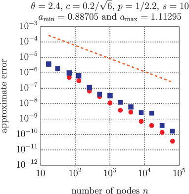


We here compare the kernel interpolation errors using both the SPOD weights (22) and serendipitous weights (24). The computed quantity in each case is the estimated error with respect to both the domain and stochastic variables, given by (6).
The results are displayed in Figures 1, 2 and 3 for the three different values, ranging from the easiest to the hardest. In each case the graphs on the left are for dimension , those on the right for . Each figure also gives the computed errors for two different values of the parameter , with the easier (i.e., smaller) value used in the upper pair, the harder (i.e., larger) value in the lower pair. Each graph also shows (dashed line) the theoretical convergence rate (21) for the given value of .
The striking fact is that the serendipitous weights perform about as well as SPOD weights for all the easier cases (all graphs in Figure 1, the upper graphs in Figures 2 and 3), while dramatically outperforming the SPOD weights for the harder cases (the lower graphs in Figures 2 and 3).
One way to assess the hardness of a particular parameter set is to inspect the values of and given in the legend above each graph. In particular, the hardest problem is the fourth graph in Figure 3, where the dimensionality is , and the random field has values ranging from around 0.1 to near 2. For this case the SPOD weights are seen to fail completely. Yet even in this case the serendipitous weights perform superbly.
The plateau in the convergence graph for the SPOD weights in Figure 3 can be explained as follows: the SPOD weights in this case become very large with increasing dimension and, in consequence, the kernel interpolant becomes very spiky at the lattice points and near zero elsewhere. Thus we are effectively seeing just the norm of the target function for feasible values of .
The intuition behind the serendipitous weights is that the problem of overly large weights is overcome by omitting the factorials in the SPOD weight formula (22).
Finally, it is worth emphasizing that the construction cost with serendipitous weights is considerably cheaper than with SPOD weights. Yet the quality of the kernel interpolant appears to be just as good as or—as seen in Figures 2 and 3—dramatically better than the interpolant based on SPOD weights. Putting these two aspects together, we resolved to repeat the experiments for a still larger value of , well beyond the reach of SPOD weights.
6.3 1000-dimensional examples


Since the serendipitous weights (24) are product weights, we are able to carry out computations using much higher dimensionalities than before. We consider the previous set of three values together with the harder value of in each case, and now set the upper limit of the series (6) to be . The results are displayed in Figure 4.
The computational performance of the kernel interpolant using serendips is seen in Figure 4 to continue to be excellent even when . The method works well even for the most difficult experiment, illustrated on the bottom of Figure 4. While the pre-asymptotic regime is even longer than in the case (shown in the bottom right of Figure 3), the kernel interpolation error does not stall as it does in the case for SPOD weights. Thus the kernel interpolant based on serendipitous weights appears to be robust in practice.
7 Conclusions
We have introduced a new class of product weights, called the serendipitous weights, to be used in conjunction with the lattice-based kernel interpolant presented in [20]. Numerical experiments illustrate that this family of weights appears to be robust when it comes to kernel interpolation of parametric PDEs.
Numerical experiments in the paper comparing the performance with previously studied SPOD weights show that not only are the new weights cheaper and easier to work with, but also they give much better results for hard problems.
Acknowledgements
F. Y. Kuo and I. H. Sloan acknowledge support from the Australian Research Council (DP210100831). This research includes computations using the computational cluster Katana [24] supported by Research Technology Services at UNSW Sydney.
References
- [1] Adcock, B., Brugiapaglia, S., Webster, C. G.: Sparse Polynomial Approximation of High-Dimensional Functions. Society for Industrial and Applied Mathematics (2022)
- [2] Bartel, F., Kämmerer, L., Potts, D., Ullrich, T.: On the reconstruction of function values at subsampled quadrature points. Preprint arXiv:2208.13597 [math.NA] (2022)
- [3] Byrenheid, G., Kämmerer, L., Ullrich, T., Volkmer, T.: Tight error bounds for rank- lattice sampling in spaces of hybrid mixed smoothness. Numer. Math. 136, 993–1034 (2017)
- [4] Cohen, A., DeVore, R.: Approximation of high-dimensional parametric PDEs. Acta Numer. 24, 1–159 (2015)
- [5] Cools, R., Kuo, F. Y., Nuyens, D., Sloan, I. H.: Lattice algorithms for multivariate approximation in periodic spaces with general weight parameters. In: Celebrating 75 Years of Mathematics of Computation (S. C. Brenner, I. Shparlinski, C.-W. Shu, and D. Szyld, eds.), Contemporary Mathematics, 754, AMS, 93–113 (2020)
- [6] Cools, R., Kuo, F. Y., Nuyens, D., Sloan, I. H.: Fast component-by-component construction of lattice algorithms for multivariate approximation with POD and SPOD weights. Math. Comp. 90, 787–812 (2021)
- [7] Dick, J., Gantner, R. N., Le Gia, Q. T., Schwab, Ch.: Higher order quasi-Monte Carlo integration for Bayesian PDE inversion. Comput. Math. Appl. 77, 144–172 (2019)
- [8] Dick, J., Kuo, F. Y., Le Gia, Q. T., Nuyens, D., Schwab, Ch.: Higher order QMC Galerkin discretization for parametric operator equations. SIAM J. Numer. Anal. 52, 2676–2702 (2014)
- [9] Dolbeault, M., Krieg, D., Ullrich, M.: A sharp upper bound for sampling numbers in . Appl. Comp. Harm. Anal. 63, 113–134 (2023)
- [10] Gantner, R. N., Herrmann, L., Schwab, Ch.: Quasi–Monte Carlo integration for affine-parametric, elliptic PDEs: local supports and product weights. SIAM J. Numer. Anal. 56, 111–135 (2018)
- [11] Gantner, R. N., Peters, M. D.: Higher-order quasi-Monte Carlo for Bayesian shape inversion. SIAM/ASA J. Uncertain. Quantif. 6, 707–736 (2018)
- [12] Gilbert, A. D., Graham, I. G., Kuo, F. Y., Scheichl, R., Sloan, I. H.: Analysis of quasi-Monte Carlo methods for elliptic eigenvalue problems with stochastic coefficients. Numer. Math. 142, 863–915 (2019)
- [13] Gilbert, A. D., Scheichl, R.: Multilevel quasi-Monte Carlo for random elliptic eigenvalue problems I: regularity and error analysis. To appear in IMA J. Numer. Anal. (2023)
- [14] Gilbert, A. D., Scheichl, R.: Multilevel quasi-Monte Carlo for random elliptic eigenvalue problems II: efficient algorithms and numerical results. To appear in IMA J. Numer. Anal. (2023)
- [15] Guth, P. A., Kaarnioja, V., Kuo, F. Y., Schillings, C., Sloan, I. H.: A quasi-Monte Carlo method for optimal control under uncertainty. SIAM/ASA J. Uncertain. Quantif. 9, 354–383 (2021)
- [16] Guth, P. A., Kaarnioja, V., Kuo, F. Y., Schillings, C., Sloan, I. H.: Parabolic PDE-constrained optimal control under uncertainty with entropic risk measure using quasi-Monte Carlo integration. Preprint arXiv:2208.02767 [math.NA] (2022)
- [17] Hakula, H., Harbrecht, H., Kaarnioja, V., Kuo, F. Y., Sloan, I. H.: Uncertainty quantification for random domains using periodic random variables. Preprint arXiv:2210.17329 [math.NA] (2022)
- [18] Harbrecht, H., Peters, M., Siebenmorgen, M.: Analysis of the domain mapping method for elliptic diffusion problems on random domains. Numer. Math. 134, 823–856 (2016)
- [19] Herrmann, L., Keller, M., Schwab, Ch.: Quasi-Monte Carlo Bayesian estimation under Besov priors in elliptic inverse problems. Math. Comp. 90, 1831–1860 (2021)
- [20] Kaarnioja, V., Kazashi, Y., Kuo, F. Y., Nobile, F., Sloan, I. H.: Fast approximation by periodic kernel-based lattice-point interpolation with application in uncertainty quantification. Numer. Math. 150, 33–77 (2022)
- [21] Kaarnioja, V., Kuo, F. Y., Sloan, I. H.: Uncertainty quantification using periodic random variables. SIAM J. Numer. Anal. 58, 1068–1091 (2020)
- [22] Kämmerer, L., Potts, D., Volkmer, T.: Approximation of multivariate periodic functions by trigonometric polynomials based on rank- lattice sampling. J. Complexity 31, 543–576 (2015)
- [23] Kämmerer, L., Volkmer, T.: Approximation of multivariate periodic functions based on sampling along multiple rank- lattices. J. Approx. Theory 246, 1–17 (2019)
- [24] Katana. Published online, DOI:10.26190/669X-A286 (2010)
- [25] Krieg, D., Ullrich, M.: Function values are enough for -approximation. Found. Comput. Math. 21, 1141–1151 (2021)
- [26] Kuo, F. Y., Mo, W., Nuyens, D.: Constructing embedded lattice-based algorithms for multivariate function approximation with a composite number of points. Preprint arXiv:2209.01002 [math.NA] (2022)
- [27] Kuo, F. Y., Nuyens, D.: Application of quasi-Monte Carlo methods to elliptic PDEs with random diffusion coefficients – a survey of analysis and implementation. Found. Comput. Math. 16, 1631–1696 (2016)
- [28] Kuo, F. Y., Nuyens, D.: Application of quasi-Monte Carlo methods to PDEs with random coefficients – an overview and tutorial. In: A. B. Owen, P. W. Glynn (eds.), Monte Carlo and Quasi-Monte Carlo Methods 2016, pp. 53–71. Springer (2018)
- [29] Kuo, F. Y., Schwab, Ch., Sloan, I. H.: Quasi-Monte Carlo finite element methods for a class of elliptic partial differential equations with random coefficients. SIAM J. Numer. Anal. 50, 3351–3374 (2012)
- [30] Kuo, F. Y., Sloan, I. H., Woźniakowski, H.: Lattice rules for multivariate approximation in the worst case setting. In: H. Niederreiter, D. Talay (eds.), Monte Carlo and Quasi-Monte Carlo Methods 2004, pp. 289–330. Springer (2006)
- [31] Nagel, N., Schäfer, M., Ullrich, T.: A new upper bound for sampling numbers. Found. Comput. Math. 22, 445–468 (2022)
- [32] Sloan, I. H., Woźniakowski., H.: Tractability of multivariate integration for weighted Korobov classes. J. Complexity 17, 697–721 (2001)
- [33] Xiu, D., Karniadakis, G. E.: The Wiener–Askey polynomial chaos for stochastic differential equations. SIAM J. Sci. Comput. 24, 619–644 (2002)
- [34] Zeng, X. Y., Leung, K. T., Hickernell, F. J.: Error analysis of splines for periodic problems using lattice designs. In: H. Niederreiter, D. Talay (eds.), Monte Carlo and Quasi-Monte Carlo Methods 2004, pp. 501–514. Springer (2006)
- [35] Zeng, X. Y., Kritzer, P., Hickernell, F. J.: Spline methods using integration lattices and digital nets. Constr. Approx. 30, 529–555 (2009)