Lateral inhibition in relaxation oscillators provides a basis for computation
Abstract
Coupled relaxation oscillators, realized via chemical or other means, can exhibit a multiplicity of steady states, characterized by spatial patterns resulting from lateral inhibition. We show that perturbation-initiated transformations between these configurations, mapped to binary strings via coarse-graining, provide a basis for computation. The rules governing these transitions emerge from an underlying effective energy landscape shaped by the global and local stabilities of these states. Our results suggest a framework by which far-from-equilibrium systems may encode a computational logic.
Complex spatio-temporal patterns seen in natural phenomena, ranging from the intricate symmetric geometry of snowflakes [1] to the development of form in multicellular organisms [2, 3, 4] and large-scale plankton patchiness in oceanic algal blooms [5, 6, 7], are associated with processes that are typically far from equilibrium [8, 9]. The behavior of the dissipative systems where such patterns arise can be described using a dynamical framework, yielding solutions ranging from waves, breathers, and solitons, to chaos [10, 11]. Each of the collective states, which are characterized by distinct emergent phenomena, encodes information about the instantaneous configuration of the system. Consequently, a transition from one pattern to another can be viewed as a “computation” that results in the transformation of such information [12, 13, 14]. Indeed, the dynamical evolution of systems such as spin glasses, which flow down rugged energy landscapes to one of many possible local minima [15], have been used to implement neural network-inspired computation [16, 17]. This paradigm has been successfully used to model brain function [18] as well as to provide innovative solutions to hard combinatorial optimization problems [19, 20, 21]. However, it has been challenging to formulate such a language, which connects dynamics and computation, for describing systems that are far from equilibrium.
In this paper, we present a framework for uncovering the computational logic of systems undergoing transitions between multiple non-equilibrium steady states. Two archetypes of the irreversible processes that characterize far-from-equilibrium systems are diffusion and chemical reactions (such as combustion) occurring in open systems [22]. Apart from being fundamental natural processes, they play important roles in biology, for instance, allowing transportation of molecules via diffusion, and their synthesis and replication through metabolic reactions [23]. Reaction-diffusion systems, in which spatio-temporal patterns can emerge through self-organization [24, 25], provide a natural framework for describing information processing in terms of out-of-equilibrium dynamics. Indeed, systems embodying these principles, such as oscillating chemical reactions and slime molds, have been used to implement specific computational algorithms [26, 27, 28, 29, 30, 31, 32]. Computation in these systems is implemented by the dynamical evolution of the initial (input) state to the final (output) state. The general computational logic presented here suggests that these algorithms belong to a much broader paradigm, in which such evolutions can be completely specified by a set of transformation rules (logic) that map the set of non-equilibrium steady states of the system to itself. By altering the perturbations applied to the system, the logic can be changed, allowing different types of computations to be realized (analogous to programming a computer). This can potentially address a central problem in biology: how living organisms “compute”, i.e., process information vital for survival through biochemical means [33, 34].
As chemical reactions occurring inside living organisms exhibit temporal recurrence across scales, we illustrate this paradigm using a generic non-equilibrium system of relaxation oscillators that are coupled diffusively. The resulting collective dynamics generates a variety of spatiotemporal patterns depending on kinetic rates and coupling strengths [35, 36, 37]. Unlike previous attempts at implementing computation in a reaction-diffusion framework, which typically involve interactions between traveling waves [38, 33, 39, 40], we use a temporally invariant, spatially heterogeneous non-equilibrium steady state. Such Spatially Patterned Oscillator Death (SPOD) states are observed for relatively strong coupling between oscillators [36]. The temporal invariance allows a particularly succinct dynamical description, and we show that a potentially infinite number of phase space trajectories resulting from different initial conditions reduce to a finite number of qualitatively distinct states. This allows coarse-graining of the state space continuum to a discrete set that can be mapped to distinct binary sequences. The time-evolution of the system thereby reduces to operations in which symbolic strings are transformed to one another. In analogy with computation in a Turing machine [41], here binary strings representing the initial and final states are the input and output, respectively, while the role of the program is played by the transformation-inducing perturbation, viz., the binary pattern of stimuli (i.e., on/off) applied to the array of oscillators. We generate a comprehensive taxonomy of the states, investigate their local, as well as, global stabilities, and provide a complete catalogue of perturbation-induced transitions between them, yielding a fundamental template for realizing computation through the collective dynamics of non-equilibrium systems.
To describe the dynamics of each node in the system of coupled relaxation oscillators, we have used a generic model for such oscillators, viz., the FitzHugh-Nagumo (FHN) equations. This model comprises a fast activation variable and a slow inactivation variable evolving as
| (1) | ||||
where the parameters and describe the kinetics, governs the recovery rate and characterizes the asymmetry of the limit cycle dynamics. The simplest coupling topology that allows the system to be used for computation is that of a one-dimensional (-D) array, as each distinct state can be mapped to a symbolic sequence by using appropriate thresholds. In this paper we have investigated a -D system of coupled oscillators with different boundary conditions, corresponding to a chain and a ring. Following Ref. [36], we consider the oscillators to be coupled by diffusion exclusively via the inactivation variable . Such a coupling captures the essence of the physical process underlying experiments in microfluidic devices [35], where the beads containing the oscillating chemical reactants are suspended in an inert medium that allows only the inhibitory species to diffuse. A linear chain with passive elements at the boundary [Fig. 1 (a)] approximates the geometry of such experimental systems, taking into account the presence of the inert medium [36]. The dynamics of the resultant system is described by:
| (2) |
where (, unless specified otherwise). The boundary conditions are specified by The diffusion coefficient denotes the strength of coupling between the inactivation variables of neighboring relaxation oscillators [42].
The effect of external stimulation on a node of the system, such as optical illumination in the case of light-sensitive chemical reactions that can initiate oscillatory activity in the medium [43], is incorporated through the term which is assumed to be constant for the duration of stimulation. In the simulations reported here, the signal intensity is assumed to be the same () for all nodes. Varying and the stimulation duration allows us to investigate the effect of signal strength on the collective dynamics. A stimulation protocol is defined by the choice of nodes (=) for which corresponding to a total of possible protocols. In principle, these protocols can implement logic gates. Indeed, we explicitly show that a conservative logic gate [44] that is capable of universal computation, can be realized using such protocols [45]. We have verified that the results reported in this paper are robust with respect to different choices of , as well as, small changes in , and .


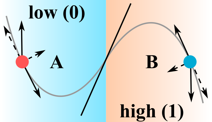
Fig. 1 (b) shows the system (2) converging to a characteristic SPOD state, marked by a temporally invariant pattern of high and low values for , as well as, (). Note that, a low (high) value of implies a low (high) value of for each element, and vice versa. For each SPOD state, all elements that are low have exactly the same numerical value for (and ), as do all elements that are high. The configuration can hence be mapped to a binary sequence using an appropriate threshold. As the steady-state probability distributions of (estimated from realizations) have a clearly bimodal form, we choose a threshold (viz., ) from the region between the peaks, our results being robust with respect to this choice. To allow an arbitrary binary string to be used as the initial state of the system [e.g., as in Fig. 1 (c)], we map the entries () of the string to the values that occur at the two peaks of the distributions (viz., and ).
The system exhibits multistability, i.e., for a given choice of parameter values, it can converge to any one of multiple possible SPOD states, each having a corresponding binary representation. Fig. 1 (c) shows an example of how one such binary string can be transformed to another through an external perturbation - a property that is vital for the system to be used for computation. While, in principle, a system of elements should be able to represent binary strings, only a small fraction of these can actually be obtained. For example, we observe only distinct strings for a chain of oscillators, and distinct strings for a ring of the same size (which reduces to on considering the cyclic permutations to be identical, taking into account the periodic boundary condition). This restriction arises from the physical mechanism by which SPOD states are generated, and can be understood by considering a pair of coupled oscillators. When the two oscillators are in opposite branches [Fig. 1 (d), right], the forces arising from diffusion and intrinsic kinetics acting on the oscillators are balanced under strong coupling, resulting in either a - or a - state [36]. For a -D array of coupled oscillators, we observe that the SPOD states contain at most two consecutive 0s or 1s, hence limiting the number of observable binary strings.
The instability of sequences containing long () contiguous blocks of 0s or 1s, for the range of we use, arises because the diffusion term for the interior node(s) in such a block is negligible (thereby disrupting the balance of forces responsible for the arrest of oscillations). Thus, these nodes effectively become uncoupled and hence oscillate, destabilizing any time-invariant states containing such blocks [45]. This also implies that SPOD states that begin or end with ‘00’ or ‘11’ will not be observed in a chain with passive elements at its ends [45]. We note also that the inversion of an observed SPOD state, obtained by exchanging s with s and vice versa, yields another allowed SPOD state. The stability of two coupled oscillators arrested in a low and a high activity state suggests that if such pairs can completely tile the entire sequence represented by the array [Fig. 1 (d), left], the pattern will be stable. Indeed, we observe that all SPOD states observed in system (2) can be viewed as a sequence of stable pairs of adjacent oscillators, each pair comprising one oscillator arrested in a high and the other in a low activity state (i.e., ‘01’ or ‘10’). This provides a basis for viewing the system as an anti-ferromagnetic spin chain (spin up/down corresponding to high/low activity), allowing us to formulate an effective energy function for the system (see below).
A simple combinatorial argument allows us to obtain the number of distinct SPOD states appearing in a chain of oscillators, , the -th term of the Fibonacci sequence [45]. For a ring, a more involved combinatorial argument is required to determine the distinct number of SPOD states, which in this case is the number of cyclic strings with at most two consecutive 0s and 1s anywhere in the string. For a system of size , this number is the coefficient of the generating function obtained using the Goulden-Jackson cluster method [46, 45]. Thus, , , and for , where and . Taking into account the periodic boundary conditions of the ring and using Polya enumeration theory [46], the number of strings unique under cyclic permutations is obtained as where and for . Here is the Euler’s totient function (or phi function) defined as the number of positive integers and relatively prime to . A numerical evaluation of these formulae show that the number of distinct SPOD states increases exponentially with system size , independent of the connection topology [45].

We now investigate the effect of perturbing the SPOD states that occur in a ring of elements by using each of the possible stimulation protocols. Fig. 2 (a) shows the perturbation-induced transitions between strings corresponding to the distinct states (invariant under cyclic permutations) for . The number of s present in a string indicates its relative stability, measured in terms of the number of transitions that originate from, or terminate at, the string. In particular, strings with the maximum (minimum) allowed number of s, i.e., () for , act as sinks (sources, respectively), although sources and sinks having zeros do also occur in this case. The maximum number of s allowed in a binary string of length , subject to the constraint that substrings of contiguous 0s (or 1s) of length are not allowed, is equal to the largest integer , while the minimum number of s allowed is . Note that the strings that are most frequently obtained when starting from random initial conditions [the largest nodes in Fig. 2 (a)] are not necessarily the ones most stable to perturbation. This difference between (i) the probability that a particular string results from perturbing the allowed states, and (ii) its basin size, i.e., the probability of obtaining the string from random initial conditions, can be understood in terms of the distinction between local and global stabilities.
The local stability of a string can be quantified in terms of the decay rate of perturbations to the corresponding SPOD state, which is related to the largest eigenvalue of the Jacobian obtained by linearizing Eqn. (2) around this state. As seen from Fig. 2 (b), strings that have the highest (and hence are sinks), are associated with the most negative values of , implying that they have much higher local stability compared to sources, i.e., strings having the lowest . The global stability of each string can be defined in terms of an energy function using the mapping to an anti-ferromagnetic spin chain. Identifying the () in the th node of a string with or “up” ( or “down”, respectively) for the corresponding spin, the associated energy is defined as (periodic boundaries imply ). Thus, states containing adjacent spins in the same orientation would have a higher energy, decreasing the likelihood that they will emerge from an arbitrary initial state and hence reducing their basin size [Fig. 2 (c)]. The use of an energy landscape to describe the system dynamics is consistent with trajectories initiated from each of the states converging to absorbing (sink) states, whose existence implies the absence of periodic cycles.
To conclude, the results presented here point to a new computing paradigm involving the global nonlinear response of a continuous medium to local perturbations, which is coordinated through diffusive transport. Our results could be verified in an experimental set-up with photoperturbations applied to arrays of light-sensitive chemical droplets in microfluidic devices [35, 43, 47]. As our model is generic, it may also be possible to execute such a computation scheme in other experimental systems involving coupled relaxation oscillators [48], including engineered bioelectric tissues [49], phototactic Physarum plasmodium [50] and insulator-metal state transition devices [51]. Considering strong inhibition between neighboring units allows us to use time-invariant patterns as the fundamental states in computation involving reaction-diffusion, instead of relying on interactions between traveling waves [40]. As there are many biological processes which involve lateral inhibition between elements having rhythmic activity that can be modeled as relaxation oscillators [52], the framework we present here may offer insights into how computation may be implemented in living systems [53].
Acknowledgements.
We would like to thank Alfred A. Aureate and Subinay Dasgupta for helpful discussions. The simulations required for this work were supported by IMSc High Performance Computing facility (hpc.imsc.res.in) [Nandadevi and Satpura], which is partially funded by the Department of Science & Technology, Government of India. This research has been supported in part by the IMSc Complex Systems Project (12th Plan), and the Center of Excellence in Complex Systems and Data Science, both funded by the Department of Atomic Energy, Government of India.References
- [1] J. S. Langer, Rev. Mod. Phys. 52, 1 (1980).
- [2] A. J. Koch and H. Meinhardt, Rev. Mod. Phys. 66, 1481 (1994).
- [3] S. Kondo and T. Miura, Science 329, 1616 (2010).
- [4] A. D. Lander, Cell 144, 955 (2011).
- [5] J. F. Gower K. L. Denman, and R. J. Holyer, Nature (Lond.) 288, 157 (1980).
- [6] E. R. Abraham, C. S. Law, P. W. Boyd, S. J. Lavender, M. T. Maldonado, and A. R. Bowie, Nature (Lond.) 407, 727 (2000).
- [7] Z. Neufeld, Phys. Rev. Lett. 87, 108301 (2001).
- [8] M. C. Cross and P. C. Hohenberg, Rev. Mod. Phys. 65, 851 (1993).
- [9] J. P. Gollub and J. S. Langer, Rev. Mod. Phys. 71, S396 (1999).
- [10] A. Hagberg, E. Meron, I. Rubinstein, and B. Zaltzman, Phys. Rev. Lett. 76, 427 (1996).
- [11] D. Haim, G. Li, Q. Ouyang, W. D. McCormick, H. L. Swinney, A. Hagberg, and E. Meron, Phys. Rev. Lett. 77, 190 (1996).
- [12] S. Wolfram, Phys. Rev. Lett. 54, 735 (1985).
- [13] J. P. Crutchfield, Nat. Phys. 8, 17 (2012).
- [14] G. De las Cuevas and T. S. Cubitt, Science 351, 1180 (2016).
- [15] M. Gu and Á. Perales, Phys. Rev. E 86, 011116 (2012).
- [16] J. J. Hopfield and D. W. Tank, Science 233, 625 (1986).
- [17] S. Becker, Y. Zhang, and A. A. Lee, Phys. Rev. Lett. 124, 108301 (2020).
- [18] D. J. Amit, Modeling Brain Function (Cambridge University Press, Cambridge, 1989).
- [19] S. Kirkpatrick, C. D. Gelatt, and M. P. Vecchi, Science 220, 671 (1983).
- [20] Y. Fu and P. W. Anderson, J. Phys. A 19, 1605 (1986).
- [21] R. Monasson, R. Zecchina, S. Kirkpatrick, B. Selman, and L. Troyansky, Nature (Lond.) 400, 133 (1999).
- [22] S. Sinha and S. Sridhar, Patterns in Excitable Media (CRC Press, Boca Raton, FL, 2015).
- [23] R. Phillips, J. Kondev, J. Theriot, H. Garcia, and N. Orme, Physical Biology of the Cell, 2nd ed. (Garland Science, New York, 2012).
- [24] A. M. Turing, Philos. Trans. R. Soc. B 237, 37 (1953).
- [25] P. Gray and S. K. Scott, Chemical Oscillations and Instabilities (Clarendon Press, Oxford, 1994).
- [26] O. Steinbock, Á. Tóth and K. Showalter, Science 267, 868 (1995).
- [27] I. R. Epstein, Science 315, 775 (2007).
- [28] J. Holley, I. Jahan, B. De Lacy Costello, L. Bull, and A. Adamatzky, Phys. Rev. E 84, 056110 (2011).
- [29] T. Nakagaki, H. Yamada, and Á. Tóth, Nature (Lond.) 407, 470 (2000).
- [30] A. Takamatsu, R. Tanaka, H. Yamada, T. Nakagaki, T. Fujii, and I. Endo, Phys. Rev. Lett. 87, 078102 (2001).
- [31] A. Tero, S. Takagi, T. Saigusa, K. Ito, D. P. Bebber, M. D. Fricker, K. Yumiki, R. Kobayashi, and T. Nakagaki, Science 327, 439 (2010).
- [32] A. Adamatzky, Physarum Machines: Computers from Slime Mould (World Scientific, Singapore, 2010).
- [33] A. Hjelmfelt, E. D. Weinberger, and J. Ross, Proc. Natl. Acad. Sci. USA 88, 10983 (1991).
- [34] A. Tamsir, J. J. Tabor, and C. A. Voigt, Nature (Lond.) 469, 212 (2011).
- [35] M. Toiya, V. K. Vanag, and I. R. Epstein, Angew. Chem. 47, 7753 (2008).
- [36] R. Singh and S. Sinha, Phys. Rev. E 87, 012907 (2013).
- [37] S. N. Menon and S. Sinha, Proc. 10th IEEE Intl. Conf. Signal Processing (2014).
- [38] O. E. Rössler, in Physics and Mathematics of the Nervous System (Lecture Notes in Biomathematics 4, edited by M. Conrad, W. Güttinger, and M. Dal Cin (Springer, Berlin, 1974), p. 399.
- [39] O. Steinbock, P. Kettunen, and K. Showalter, J. Phys. Chem. 100, 18970, (1996).
- [40] A. Adamatzky, Phil. Trans. R. Soc. B 374, 20180372 (2019).
- [41] J. E. Hopcroft, R. Motwani, and J. Ullman, Introducation to Automata Theory, Languages, and Computation, 2nd ed. (Addison-Wesley, Reading, Mass., 2001).
- [42] This choice of the coupling strength ensures that a system of oscillators described by Eqn. 2 converges to SPOD states, see Ref. [36].
- [43] V. Gáspár, G. Basza and M. T. Beck, Z. Phys. Chemie 264, 43 (1983).
- [44] E. Fredkin, and T. Toffoli, Int. J. Theor. Phys. 21, 219 (1982).
- [45] See Supplementary Information.
- [46] A. E. Edlin, and D. Zeilberger, Adv. Appl. Math. 25, 228 (2000).
- [47] J. Delgado, N. Li, M. Leda, H. O. González-Ochoa, S. Fraden, and I. R. Epstein, Soft Matter 7, 3155 (2011).
- [48] L. V. Gambuzza, A. Buscarino, S. Chessari, L. Fortuna, R. Meucci, and M. Frasca, Phys. Rev. E 90 , 032905 (2014).
- [49] H. M. McNamara, H. Zhang, C. A. Werley, and A. E. Cohen, Phys. Rev. X 6, 031001 (2016).
- [50] T. Nakagaki, H. Yamada, and T. Ueda, Biophys. Chem. 82, 23 (1999).
- [51] A. Parihar, N. Shukla, M. Jerry, S. Datta, and A. Raychowdhury, Nanophotonics 6, 601 (2017).
- [52] R. Janaki, S. N. Menon, R. Singh, and S. Sinha, Phys. Rev. E 99, 052216 (2019).
- [53] A. Brabazon, M. O’Neill, and S. McGarraghy, Natural Computing Algorithms (Springer, Berlin, 2015).
SUPPLEMENTARY INFORMATION
Lateral inhibition in relaxation oscillators provides a basis for computation
A. Parveena Shamim, Shakti N. Menon and Sitabhra Sinha
List of Supplementary Figures
-
1.
Fig S1: Stylized representation of the attractors of the dynamical system comprising a chain of relaxation oscillators diffusively coupled with .
-
2.
Fig S2: Statistics of the binary strings corresponding to the attractors for the dynamical system comprising linearly coupled relaxation oscillators.
-
3.
Fig S3: Generation procedure for binary strings of length representing the allowed SPOD configurations in a system of oscillators arranged in a chain topology.
-
4.
Fig S4: Dependence of the number of binary strings on the size of the system for three distinct cases.
-
5.
Fig S5: Alternative representation of the transitions shown in Fig. 2 (a) of the main text.
-
6.
Fig S6: Networks showing the transitions that occur upon perturbing SPOD states in a ring of oscillators.
-
7.
Fig S7: Implementation of a Fredkin gate using a given perturbation protocol.
I Numerical details
The dynamical equations [Eqn. (2) of the main text] are solved using a fourth order Runge-Kutta scheme with time step dimensionless units. Time is expressed in units of the period of an uncoupled oscillating element. The initial conditions for each element are randomly sampled from the limit cycle of an uncoupled oscillator. The simulations reported here use boundary conditions that correspond to either the chain topology described in the main text [i.e., ], or a ring [i.e., , ].
The choices of the parameters governing the external stimulation, viz., the signal intensity and the duration for which it is applied, are constrained to an extent by the requirement that the qualitative nature of the collective dynamics should not be altered as a result (i.e., a steady state configuration upon perturbation should converge to another steady state, rather than a spatio-temporally varying pattern).
We note that for much higher values of (e.g., ) it is possible to observe contiguous blocks of s or s having length , in particular, and , but the variable does not have a clear bimodal distribution in this case. Hence, an unambiguous mapping of the physical state to a binary string may not be possible for such stronger coupling scenarios.
The absence of SPOD states beginning or ending with ‘00’ or ‘11’ in a chain having passive elements at its ends, is a consequence of the boundary condition. As the the passive elements at the edges will assume the same activity state (low or high) as that of its neighboring oscillator, this effectively results in a block of three consecutive s or s that destabilizes the time-invariant SPOD state to which it belongs.

Fig. S1 shows all the 68 distinct SPOD configurations (represented as binary strings, see main text for details about the corresponding mapping) obtained as attractors of the dynamics for a chain of oscillators, out of the possible binary states that the system can adopt during its time-evolution. The statistics for the attractors, including estimates of the sizes of their basins of attraction, are obtained by performing different realizations of the system dynamics using randomly chosen initial configurations.

II Reading Frames
In Fig. 1 (d, left) in the main text we have shown the tiling of a chain of oscillators by stable pairs of adjacent oscillators arrested in low and high activity states, respectively. Note that when we use such oscillator pairs to tile the chain without any overlaps, (using pairs for any chain of length that can be completely tiled), there are two possible reading frames, starting from odd and even numbered sites, respectively. The most frequently occurring configurations, viz., those comprising a strictly alternating sequence of 0s and 1s (see, e.g., Fig. S1 for ), can be completely tiled by contiguous stable pairs in either of the reading frames. In contrast, sequences containing adjacent oscillators in the same activity state, viz. ‘00’ or ‘11’, can be completely tiled in at most one of the reading frames (see Fig. S2 for a graphical overview of the statistics of strings with such ‘defects’). For sequences in which neither reading frame leads to a complete tiling, switching between the frames can achieve this [see, e.g., Fig. 1 (d), left, in main text]. The number of nodes that can be tiled using stable oscillator pairs in both reading frames (which has a maximum value of ) provides a measure of the stability of the sequence. In particular, if the string corresponding to a state cannot be completely tiled under both reading frames, then the state will not be stable, and hence will not be observed.
III Number of binary strings in different connection topologies
We provide below combinatorial arguments for obtaining the number of distinct SPOD configurations represented using binary strings in a 1-dimensional array of oscillators with different boundary conditions.
III.1 Chain of oscillators
To calculate the number of SPOD configurations in a chain (i.e., where the oscillators can be uniquely identified in terms of their position in the sequence in which they occur in the array), we note that this can be expressed by first finding the number of binary strings of length which do not contain more than two consecutive s or s (as this is disallowed under the system dynamics for the parameter values used). We then remove from this set all strings, say in number, which have two consecutive s or s at either boundary of the chain (as the boundary conditions prevent the dynamics at the chain ends from generating such patterns). For a given , the number is simply obtained by counting the strings generated using a pair of binary trees, one beginning with and the other with at its root, and terminating at level , subject to the constraint that the strings of length , obtained by following along every branch the binary digits occurring at each level from the root (level ) to leaf (level ), should not have more than two consecutive s or s. As can be seen from Fig. S3, the number of such sequences for each of the two binary trees is given by , i.e., the ()-th Fibonacci number (, , , , …). As the two binary trees are identical with only and interchanged, this implies that . Similar arguments yield . Thus, the total number of SPOD states for oscillators arranged in a chain topology is .

III.2 Ring comprising oscillators
We now obtain the number of distinct SPOD configurations in a ring topology, i.e., which are invariant under cyclic permutations. Using Goulden-Jackson cluster method, the generating function for the number of cyclic strings is:
| (3) | ||||
where . The coefficients of are in general given by:
| (4) |
where and .

The number of strings unique under cyclic permutations is
| (5) |
where
| (6) | ||||
and is the Euler’s totient function (or phi function) defined as the number of positive integers and relatively prime to .
Fig. S4 shows for different topologies, viz., the chain and the ring, the nature of increase in the number of distinct SPOD configurations.
IV Perturbation-induced transitions
As mentioned in the main text, perturbing a SPOD state in an array of coupled oscillators, using any one of the possible protocols for stimulating the various distinct possible combinations of oscillators, results in the system converging to any of the dynamical attractors (corresponding to distinct SPOD states). Fig. 2 (a) in the main text represents the entire set of such perturbation-induced transitions between the 14 possible distinct SPOD states in a system of oscillators arranged in a ring topology (diffusive coupling strength ). While the width of a directed link between two SPOD states in Fig. 2 (a) have been made proportional to the number of perturbations that drive a given input state to a given output state , in Fig. S5 we present the information about these transitions using an alternative representation that allows certain information about these transition to be gleaned more conveniently. In particular, we immediately note from Fig. S5 that of the SPOD states (viz., , , , , and ) are stable configurations, in that no perturbation applied on such a string can result in a transition to some other state.
The representation also allows us to infer the relative fraction of different perturbations of various states that converge to a particular output state by looking at the total area of blocks having the same color. For instance, Fig. S5 indicates that the stable state can be arrived at from many of the other SPOD states through the application of a large number of possible perturbations. Note that, this is quite distinct from the concept of ‘basin of attraction’ of a SPOD state , which asks how many different randomly chosen initial configurations (which need not correspond to a SPOD state) converge to . Thus, for example, in this case, the state having the largest basin size is [Fig. 2 (a)], which has fewer perturbation-induced transitions to it than the aforementioned SPOD state . This difference can be traced to the distinction between local and global stability as discussed in the main text.

We also note from Fig. S5 that input states differ in terms of the number of distinct output states that can be reached via different perturbations. While stable input states each have an unique output state (namely itself) which is independent of the perturbation applied, other states could map to a few (e.g., states and map to either themselves or to depending on the perturbation) or many output states. An example of the latter is the input state , whose perturbation-induced transitions are shown in detail in Fig. S6 (a).
In order to understand how the application of a particular perturbation to each of the distinct input states in turn results in transitions to different output states, we have considered in Fig. S6 (b) the protocol in which all oscillators are stimulated While of the states are left unchanged by the perturbation, of the remaining states map to (the state which is the target of the largest number of perturbation-induced transitions, as we have seen from Fig. S5) while one state maps to (the state having the largest basin) and the other maps to . Note that while, in general, states having the maximum number of s (nodes colored green) act as sinks and those having the minimum number (nodes colored blue) act as sources, not all such nodes behave similarly for a given perturbation. For instance, (a blue colored node) does not map to any other state under this particular stimulation protocol, while (a green colored node) is arrived at only from itself.


V Implementation of a conservative logic gate
Here we show that an array of coupled oscillators subject to a given perturbation can be used to implement a conservative logic gate, specifically the Fredkin gate, which is known to be universal (in the sense that any logical operation can be realized by suitable combinations of these gates; see Ref. [44] cited in the main text for details). Operations performed by this gate are reversible, such that the transformation of an input configuration to a given output can be inverted by connecting it to another gate, creating a cascade. The Fredkin gate is therefore its own inverse , where .

The Fredkin gate is typically represented as a gate which has input channels (, , ) and output channels (, , ), each of which have binary values ( or ). The control line is unchanged by the gate, and we identify its value as indicating either the application of a given perturbation () or not (). The input and output channels are represented as sets comprising an odd number of sites in the array ( for the results shown here). The value assigned to each channel is obtained by applying the majority rule on the states of the constituent sites. Thus, if a channel consists of three sites (i.e., ) with at least two in the state , then the value assigned to the channel is ; else it is assigned . A given pair of input and output channels , () share the same sites, such that the logical operation of the gate is identified with the state transformation resulting from the perturbation.
Fig. S7 shows a realization of the Fredkin gate using a protocol where, if the perturbation is applied (), the sites , , , and are stimulated with amplitude for a duration , while corresponds to absence of perturbation such that the state of the array remains unchanged (the panels show only the non-trivial case ). As can be seen, each of the rows of the Fredkin gate truth table for can be implemented using this perturbation. We have verified that other perturbation schemes also realize this logic.