Latent Template Induction with Gumbel-CRFs
Abstract
Learning to control the structure of sentences is a challenging problem in text generation. Existing work either relies on simple deterministic approaches or RL-based hard structures. We explore the use of structured variational autoencoders to infer latent templates for sentence generation using a soft, continuous relaxation in order to utilize reparameterization for training. Specifically, we propose a Gumbel-CRF, a continuous relaxation of the CRF sampling algorithm using a relaxed Forward-Filtering Backward-Sampling (FFBS) approach. As a reparameterized gradient estimator, the Gumbel-CRF gives more stable gradients than score-function based estimators. As a structured inference network, we show that it learns interpretable templates during training, which allows us to control the decoder during testing. We demonstrate the effectiveness of our methods with experiments on data-to-text generation and unsupervised paraphrase generation.
1 Introduction
Recent work in NLP has focused on model interpretability and controllability [63, 34, 24, 55, 16], aiming to add transparency to black-box neural networks and control model outputs with task-specific constraints. For tasks such as data-to-text generation [50, 63] or paraphrasing [37, 16], interpretability and controllability are especially important as users are interested in what linguistic properties – e.g., syntax [4], phrases [63], main entities [49] and lexical choices [16] – are controlled by the model and which part of the model controls the corresponding outputs.
Most existing work in this area relies on non-probabilistic approaches or on complex Reinforcement Learning (RL)-based hard structures. Non-probabilistic approaches include using attention weights as sources of interpretability [26, 61], or building specialized network architectures like entity modeling [49] or copy mechanism [22]. These approaches take advantages of differentiability and end-to-end training, but does not incorporate the expressiveness and flexibility of probabilistic approaches [45, 6, 30]. On the other hand, approaches using probabilistic graphical models usually involve non-differentiable sampling [29, 65, 34]. Although these structures exhibit better interpretability and controllability [34], it is challenging to train them in an end-to-end fashion.
In this work, we aim to combine the advantages of relaxed training and graphical models, focusing on conditional random field (CRF) models. Previous work in this area primarily utilizes the score function estimator (aka. REINFORCE) [62, 52, 29, 32] to obtain Monte Carlo (MC) gradient estimation for simplistic categorical models [44, 43]. However, given the combinatorial search space, these approaches suffer from high variance [20] and are notoriously difficult to train [29]. Furthermore, in a linear-chain CRF setting, score function estimators can only provide gradients for the whole sequence, while it would be ideal if we can derive fine-grained pathwise gradients [44] for each step of the sequence. In light of this, naturally one would turn to reparameterized estimators with pathwise gradients which are known to be more stable with lower variance [30, 44].
Our simple approach for reparameterizing CRF inference is to directly relax the sampling process itself. Gumbel-Softmax [27, 38] has become a popular method for relaxing categorical sampling. We propose to utilize this method to relax each step of CRF sampling utilizing the forward-filtering backward-sampling algorithm [45]. Just as with Gumbel-Softmax, this approach becomes exact as temperature goes to zero, and provides a soft relaxation in other cases. We call this approach Gumbel-CRF. As is discussed by previous work that a structured latent variable may have a better inductive bias for capturing the discrete nature of sentences [28, 29, 16], we apply Gumbel-CRF as the inference model in a structured variational autoencoder for learning latent templates that control the sentence structures. Templates are defined as a sequence of states where each state controls the content (e.g., properties of the entities being discussed) of the word to be generated.
Experiments explore the properties and applications of the Gumbel-CRF approach. As a reparameterized gradient estimator, compared with score function based estimators, Gumbel-CRF not only gives lower-variance and fine-grained gradients for each sampling step, which leads to a better text modeling performance, but also introduce practical advantages with significantly fewer parameters to tune and faster convergence ( 6.1). As a structured inference network, like other hard models trained with REINFORCE, Gumbel-CRF also induces interpretable and controllable templates for generation. We demonstrate the interpretability and controllability on unsupervised paraphrase generation and data-to-text generation ( 6.2). Our code is available at https://github.com/FranxYao/Gumbel-CRF.
2 Related Work
Latent Variable Models and Controllable Text Generation. Broadly, our model follows the line of work on deep latent variable models [14, 30, 54, 23, 11] for text generation [28, 42, 16, 67]. At an intersection of graphical models and deep learning, these works aim to embed interpretability and controllability into neural networks with continuous [7, 67], discrete [27, 38], or structured latent variables [29]. One typical template model is the Hidden Semi-Markov Model (HSMM), proposed by Wiseman et al. [63]. They use a neural generative HSMM model for joint learning the latent and the sentence with exact inference. Li and Rush [34] further equip a Semi-Markov CRF with posterior regularization [18]. While they focus on regularizing the inference network, we focus on reparameterizing it. Other works about controllability include [55, 24, 33], but many of them stay at word-level [17] while we focus on structure-level controllability.
Monte Carlo Gradient Estimation and Continuous Relaxation of Discrete Structures. Within the range of MC gradient estimation [44], our Gumbel-CRF is closely related to reparameterization and continuous relaxation techniques for discrete structures [64, 36, 31]. To get the MC gradient for discrete structures, many previous works use score-function estimators [52, 43, 29, 65]. This family of estimators is generally hard to train, especially for a structured model [29], while reparameterized estimators [30, 54] like Gumbel-Softmax [27, 38] give a more stable gradient estimation. In terms of continuous relaxation, the closest work is the differentiable dynamic programming proposed by Mensch and Blondel [40]. However, their approach takes an optimization perspective, and it is not straightforward to combine it with probabilistic models. Compared with their work, our Gumbel-CRF is a specific differentiable DP tailored for FFBS with Gumbel-Softmax. In terms of reparameterization, the closest work is the Perturb-and-MAP Markov Random Field (PM-MRF), proposed by Papandreou and Yuille [46]. However, when used for sampling from CRFs, PM-MRF is a biased sampler, while FFBS is unbiased. We will use a continuously relaxed PM-MRF as our baseline, and compare the gradient structures in detail in the Appendix.
3 Gumbel-CRF: Relaxing the FFBS Algorithm

In this section, we discuss how to relax a CRF with Gumbel-Softmax to allow for reparameterization. In particular, we are interested in optimizing for an expectation under a parameterized CRF distribution, e.g.,
| (1) |
We start by reviewing Gumbel-Max [27], a technique for sampling from a categorical distribution. Let be a categorical random variable with domain parameterized by the probability vector , denoted as . Let denotes the standard Gumbel distribution, are i.i.d. gumbel noise. Gumbel-Max sampling of can be performed as: . Then the Gumbel-Softmax reparameterization is a continuous relaxation of Gumbel-Max by replacing the hard argmax operation with the softmax,
| (2) |
where can be viewed as a relaxed one-hot vector of . As , we have .
Now we turn our focus to CRFs which generalize softmax to combinatorial structures. Given a sequence of inputs a linear-chain CRF is parameterized by the factorized potential function and defines the probability of a state sequence over .
| (3) | |||
| (4) |
The conditional probability of is given by the Gibbs distribution with a factorized potential (equation 3). The partition function can be calculated with the Forward algorithm [58] (equation 4) where is the forward variable summarizing the potentials up to step .
To sample from a linear-chain CRF, the standard approach is to use the forward-filtering backward-sampling (FFBS) algorithm (Algorithm 1). This algorithm takes and as inputs and samples with a backward pass utilizing the locally conditional independence. The hard operation comes from the backward sampling operation for at each step (line 6). This is the operation that we focus on.
We observe that is a categorical distribution, which can be directly relaxed with Gumbel-Softmax. This leads to our derivation of the Gumbelized-FFBS algorithm(Algorithm 2). The backbone of Algorithm 2 is the same as the original FFBS except for two key modifications: (1) Gumbel-Max (line 8-9) recovers the unbiased sample and the same sampling path as Algorithm 1; (2) the continuous relaxation of argmax with softmax (line 8) that gives the differentiable111 Note that argmax is also differentiable almost everywhere, however its gradient is almost 0 everywhere and not well-defined at the jumping point [48]. Our relaxed does not have these problems. (but biased) .
We can apply this approach in any setting requiring structured sampling. For instance let denote the sampled distribution and be a downstream model. We achieve a reparameterized gradient estimator for the sampled model with :
| (5) |
We further consider a straight-through (ST) version [27] of this estimator where we use the hard sample in the forward pass, and back-propagate through each of the soft .
We highlight one additional advantage of this reparameterized estimator (and its ST version), compared with the score-function estimator. Gumbel-CRF uses which recieve direct fine-grained gradients for each step from the itself. As illustrated in Figure 1 (here is the generative model), is a differentiable function of the potential and the noise: . So during back-propagation, we can take stepwise gradients weighted by the uses of the state. On the other hand, with a score-function estimator, we only observe the reward for the whole sequence, so the gradient is at the sequence level . The lack of intermediate reward, i.e., stepwise gradients, is an essential challenge in reinforcement learning [56, 66]. While we could derive a model specific factorization for the score function estimator , this challenge is circumvented with the structure of Gumbel-CRF, thus significantly reducing modeling complexity in practice (detailed demonstrations in experiments).
4 Gumbel-CRF VAE
An appealing use of reparameterizable CRF models is to learn variational autoencoders (VAEs) with a structured inference network. Past work has shown that these models (trained with RL) [29, 34] can learn to induce useful latent structure while producing accurate models. We introduce a VAE for learning latent templates for text generation. This model uses a fully autoregressive generative model with latent control states. To train these control states, it uses a CRF variational posterior as an inference model. Gumbel CRF is used to reduce the variance of this procedure.
Generative Model We assume a simple generative process where each word of a sentence is controlled by a sequence of latent states , i.e., template, similar to Li and Rush [34]:
| (6) | ||||
| (7) | ||||
| (8) | ||||
| (9) |
Where Dec denotes the decoder, FF denotes a feed-forward network, denotes the decoder state, denotes vector concatenation. denotes the embedding function. Under this formulation, the generative model is autoregressive w.r.t. both and . Intuitively, it generates the control states and words in turn, and the current word is primarily controlled by its corresponding .

Inference Model Since the exact inference of the posterior is intractable, we approximate it with a variational posterior and optimize the following form of the ELBO objective:
| (10) |
Where denotes the entropy. The key use of Gumbel-CRF is for reparameterizing the inference model to learn control-state templates. Following past work [25], we parameterize as a linear-chain CRF whose potential is predicted by a neural encoder:
| (11) | ||||
| (12) | ||||
| (13) |
Where Enc denotes the encoder and is the encoder state. With this formulation, the entropy term in equation 10 can be computed efficiently with dynamic programming, which is differentiable [39].
Training and Testing The key challenge for training is to maximize the first term of the ELBO under the expectation of the inference model, i.e.
Here we use the Gumbel-CRF gradient estimator with relaxed samples from the Gumbelized FFBS (Algorithm 2) in both the forward and backward passes. For the ST version of Gumbel-CRF, we use the exact sample in the forward pass and back-propogate gradients through the relaxed . During testing, for evaluating paraphrasing and data-to-text, we use greedy decoding for both and . For experiments controlling the structure of generated sentences, we sample a fixed MAP from the training set (i.e., the aggregated variational posterior), feed it to each decoder steps, and use it to control the generated .
Extension to Conditional Settings For conditional applications, such as paraphrasing and data-to-text, we make a conditional extension where the generative model is conditioned on a source data structure , formulated as . Specifically, for paraphrase generation, is the bag of words (a set, being the size of the BOW) of the source sentence, similar to Fu et al. [16]. We aim to generate a different sentence with the same meaning as the input sentence. In addition to being autoregressive on and , the decoder also attend to [1] and copy [22] from . For data-to-text, we denote the source data is formed as a table of key-value pairs: , N being size of the table. We aim to generate a sentence that best describes the table. Again, we condition the generative model on by attending to and copying from it. Note our formulation would effectively become a neural version of slot-filling: for paraphrase generation we fill the BOW into the neural templates, and for data-to-text we fill the values into neural templates. We assume the inference model is independent from the source and keep it unchanged, i.e., . The ELBO objective in this conditional setting is:
| (14) |
5 Experimental Setup
Our experiments are in two parts. First, we compare Gumbel-CRF to other common gradient estimators on the standard text modeling task. Then we integrate Gumbel-CRF to real-world models, specifically paraphrase generation and data-to-text generation.
Datasets We focus on two datasets. For text modeling and data-to-text generation, we use the E2E dataset[50], a common dataset for learning structured templates for text [63, 34]. This dataset contains approximately 42K training, 4.6K validation and 4.6K testing sentences. The vocabulary size is 945. For paraphrase generation we follow the same setting as Fu et al. [16], and use the common MSCOCO dataset. This dataset has 94K training and 23K testing instances. The vocabulary size is 8K.
Metrics For evaluating the gradient estimator performance, we follow the common practice and primarily compare the test negative log-likelihood (NLL) estimated with importance sampling. We also report relative metrics: ELBO, perplexity (PPL), and entropy of the inference network. Importantly, to make all estimates unbiased, all models are evaluated in a discrete setting with unbiased hard samples. For paraphrase task performance, we follow Liu et al. [37], Fu et al. [16] and use BLEU (bigram to 4-gram) [47] and ROUGE [35] (R1, R2 and RL) to measure the generation quality. We note that although being widely used, the two metrics do not penalize the similarity between the generated sentence and the input sentence (because we do not want the model to simply copy the input). So we adopt iBLUE [57], a specialized BLUE score that penalize the ngram overlap between the generated sentence and the input sentence, and use is as our primary metrics. The iBLUE score is defined as: iB, where iB denotes iBLUE score, B denotes BLUE score, denote input, output, and reference sentences respectively. We follow Liu et al. [37] and set . For text generation performance, we follow Li and Rush [34] and use the E2E official evaluation script, which measures BLEU, NIST [5], ROUGE, CIDEr [60], and METEOR [3]. More experimental details are in the Appendix.
VAE Training Details
At the beginning of training, to prevent the decoder from ignoring , we apply word dropout [7], i.e., to randomly set the input word embedding at certain steps to be 0. After converges to a meaningful local optimal, we gradually decrease word dropout ratio to 0 and recover the full model. For optimization, we add a coefficient to the entropy term, as is in the -VAE [23]. As is in many VAE works [7, 10], we observe the posterior collapse problem where converges to meaningless local optimal. We observe two types of collapsed posterior in our case: a constant posterior ( outputs a fixed no matter what is. This happens when is too weak), and a uniform posterior (when is too strong). To prevent posterior collapse, should be carefully tuned to achieve a balance.
6 Results
| Model | Neg. ELBO | NLL | PPL | Ent. | #sample |
|---|---|---|---|---|---|
| RNNLM | - | 34.69 | 4.94 | - | - |
| PM-MRF | 69.15 | 50.22 | 10.41 | 4.11 | 1 |
| PM-MRF-ST | 53.16 | 37.03 | 5.48 | 2.04 | 1 |
| REINFORCE-MS | 35.11 | 34.50 | 4.84 | 3.48 | 5 |
| REINFORCE-MS-C | 34.35 | 33.82 | 4.71 | 3.34 | 5 |
| Gumbel-CRF (ours) | 38.00 | 35.41 | 4.71 | 3.03 | 1 |
| Gumbel-CRF-ST (ours) | 34.18 | 33.13 | 4.54 | 3.26 | 1 |
6.1 Gumbel-CRF as Gradient Estimator: Text Modeling
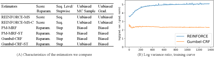
We compare our Gumbel-CRF (original and ST variant) with two sets of gradient estimators: score function based and reparameterized. For score function estimators, we compare our model with REINFORCE using the mean reward of other samples (MS) as baseline. We further find that adding a carefully tuned constant baseline helps with the scale of the gradient (REINFORCE MS-C). For reparameterized estimators, we use a tailored Perturb-and-Map Markov Random Field (PM-MRF) estimator [46] with the continuous relaxation introduced in Corro and Titov [9]. Compared to our Gumbel-CRF, PM-MRF adds Gumbel noise to local potentials, then runs a relaxed structured argmax algorithm [40]. We further consider a straight-through (ST) version of PM-MRF. The basics of these estimators can be characterized from four dimensions, as listed in Figure 3(A). The appendix provides a further theoretical comparison of gradient structures between these estimators.
Table 1 shows the main results comparing different gradient estimators on text modeling. Our Gumbel-CRF-ST outperforms other estimators in terms of NLL and PPL. With fewer samples required, reparameterization and continuous relaxation used in Gumbel-CRF are particularly effective for learning structured inference networks. We also see that PM-MRF estimators perform worse than other estimators. Due to the biased nature of the Perturb-and-MAP sampler, during optimization, PM-MRF is not optimizing the actual model. As a Monte Carlo sampler (forward pass, rather than a gradient estimator) Gumbel-CRF is less biased than PM-MRF. We further observe that both the ST version of Gumbel-CRF and PM-MRF perform better than the non-ST version. We posit that this is because of the consistency of using hard samples in both training and testing time (although non-ST has other advantages).
Variance Analysis To show that reparameterized estimators have lower variance, we compare the log variance ratio of Gumbel-CRF and REINFORCE-MS-C (Figure 3 B), which is defined as ( is gradients of the inference model)222 Previous works compare variance, rather than variance ratio [59, 19]. We think that simply comparing the variance is only reasonable when the scale of gradients are approximately the same, which may not hold in different estimators. In our experiments, we observe that the gradient scale of Gumbel-CRF is significantly smaller than REINFORCE, thus the variance ratio may be a better proxy for measuring stability. . We see that Gumbel-CRF has a lower training curve of than REINFORCE-MS, showing that it is more stable for training.
6.2 Gumbel-CRF for Control: Data-to-Text and Paraphrase Generation
Data-to-Text Generation Data-to-text generation models generate descriptions for tabular information. Classical approaches use rule-based templates with better interpretability, while recent approaches use neural models for better performance. Here we aim to study the interpretability and controllability of latent templates. We compare our model with neural and template-based models. Neural models include: D&J[13] (with basic seq2seq); and KV2Seq[15] (with SOTA neural memory architectures); Template models include: SUB[13] (with rule-based templates); hidden semi-markov model (HSMM)[63] (with neural templates); and another semi-markov CRF model (SM-CRF-PC)[34] (with neural templates and posterior regularization[18]).
Table 2 shows the results of data-to-text generation. As expected, neural models like KV2Seq with advanced architectures achieve the best performance. Template-related models all come with a certain level of performance costs for better controllability. Among the template-related models, SM-CRF PC performs best. However, it utilizes multiple weak supervision to achieve better template-data alignment, while our model is fully unsupervised for the template. Our model, either trained with REINFORCE or Gumbel-CRF, outperforms the baseline HSMM model. We further see that in this case, models trained with Gumbel-CRF gives better end performance than REINFORCE.
| Model | BLEU | NIST | ROUGE | CIDEr | METEOR |
|---|---|---|---|---|---|
| D&J[13] | 65.93 | 8.59 | 68.50 | 2.23 | 44.83 |
| KV2Seq[15] | 74.72 | 9.30 | 70.69 | 2.23 | 46.15 |
| SUB[13] | 43.78 | 6.88 | 54.64 | 1.39 | 37.35 |
| HSMM[63] | 55.17 | 7.14 | 65.70 | 1.70 | 41.91 |
| HSMM-AR[63] | 59.80 | 7.56 | 65.01 | 1.95 | 38.75 |
| SM-CRF PC [34] | 67.12 | 8.52 | 68.70 | 2.24 | 45.40 |
| REINFORCE | 60.41 | 7.99 | 62.54 | 1.78 | 38.04 |
| Gumbel-CRF | 65.83 | 8.43 | 65.06 | 1.98 | 41.44 |


To see how the learned templates induce controllability, we conduct a qualitative study. To use the templates, after convergence, we collect and store all the MAP for the training sentences. During testing, given an input table, we retrieve a template and use this as the control state for the decoder. Figure 4 shows sentences generated from templates. We can see that sentences with different templates exhibit different structures. E.g,. the first sentence for the clowns coffee shop starts with the location, while the second starts with the price. We also observe a state-word correlation. E.g,. state 44 always corresponds to the name of a restaurant and state 8 always corresponds to the rating.
To see how learned latent states encode sentence segments, we associate frequent -state ngrams with their corresponding segments (Figure 5). Specifically, after the convergence of training, we: (a) collect the MAP templates for all training cases, (b) collapse consecutive states with the same class into one single state (e.g., a state sequence [1, 1, 2, 2, 3] would be collapsed to [1, 2, 3]), (c) gather the top 100 most frequent state ngrams and their top5 corresponding sentence segments, (d) pick the mutually most different segments (because the same state ngram may correspond to very similar sentence segments, and the same sentence segment may correspond to different state ngrams). Certain level of cherry picking happens in step (d). We see that state ngrams have a vague correlation with sentence meaning. In cases (A, B, D, E), a state ngram encode semantically similar segments (e.g., all segments in case A are about location, and all segments in case E are about food and price). But the same state ngram may not correspond to the same sentence meaning (cases C, F). For example, while (C1) and (C2) both correspond to state bigram 20-12, (C1) is about location but (C2) is about comments.
Unsupervised Paraphrase Generation Unsupervised paraphrase generation is defined as generating different sentences conveying the same meaning of an input sentence without parallel training instances. To show the effectiveness of Gumbel-CRF as a gradient estimator, we compare the results when our model is trained with REINFORCE. To show the overall performance of our structured model, we compare it with other unsupervised models, including: a Gaussian VAE for paraphrasing [7]; CGMH [41], a general-purpose MCMC method for controllable generation; UPSA [37], a strong paraphrasing model with simulated annealing. To better position our template model, we also report the supervised performance of a state-of-the-art latent bag of words model (LBOW) [16].
| Model | iB4 | B2 | B3 | B4 | R1 | R2 | RL |
|---|---|---|---|---|---|---|---|
| LBOW [16] | - | 51.14 | 35.66 | 25.27 | 42.08 | 16.13 | 38.16 |
| Gaussian VAE[7] | 7.48 | 24.90 | 13.04 | 7.29 | 22.05 | 4.64 | 26.05 |
| CGMH [41] | 7.84 | - | - | 11.45 | 32.19 | 8.67 | - |
| UPSA [37] | 9.26 | - | - | 14.16 | 37.18 | 11.21 | - |
| REINFORCE | 11.20 | 41.29 | 26.54 | 17.10 | 32.57 | 10.20 | 34.97 |
| Gumbel-CRF | 10.20 | 38.98 | 24.65 | 15.75 | 31.10 | 9.24 | 33.60 |
Table 3 shows the results. As expected, the supervised model LBOW performs better than all unsupervised models. Among unsupervised models, the best iB4 results come from our model trained with REINFORCE. In this task, when trained with Gumbel-CRF, our model performs worse than REINFORCE (though better than other paraphrasing models). We note that this inconsistency between the gradient estimation performance and the end task performance involve multiple gaps between ELBO, NLL, and BLEU. The relationship between these metrics may be an interesting future research direction.
| Model | Hyperparams. | #s | GPU mem | Sec. per batch |
|---|---|---|---|---|
| REINFORCE | 5 | 1.8G | 1.42 | |
| Gumbel-CRF | 1 | 1.1G | 0.48 |
Practical Benefits Although our model can be trained on either REINFORCE or Gumbel-CRF, we emphasize that training structured variables with REINFORCE is notoriously difficult [34], and Gumbel-CRF substantially reduces the complexity. Table 4 demonstrates this empirically. Gumbel-CRF requires fewer hyperparameters to tune, fewer MC samples, less GPU memory, and faster training. These advantages would considerably benefit all practitioners with significantly less training time and resource consumption.
7 Conclusion
In this work, we propose a pathwise gradient estimator for sampling from CRFs which exhibits lower variance and more stable training than existing baselines. We apply this gradient estimator to the task of text modeling, where we use a structured inference network based on CRFs to learn latent templates. Just as REINFORCE, models trained with Gumbel-CRF can also learn meaningful latent templates that successfully encode lexical and structural information of sentences, thus inducing interpretability and controllability for text generation. Furthermore, the Gumbel-CRF gives significant practical benefits than REINFORCE, making it more applicable to real-world tasks.
Broader Impact
Generally, this work is about controllable text generation. When applying this work to chatbots, one may get a better generation quality. This could potentially improve the accessibility [8, 53] for people who need a voice assistant to use an electronic device, e.g. people with visual, intellectual, and other disabilities [51, 2]. However, if not properly tuned, this model may generate improper sentences like fake information, putting the user at a disadvantage. Like many other text generation models, if trained with improper data (fake news [21], words of hatred [12]), a model could generate these sentences as well. In fact, one of the motivations for controllable generation is to avoid these situations [63, 12]. But still, researchers and engineers need to be more careful when facing these challenges.
References
- Bahdanau et al. [2015] Dzmitry Bahdanau, Kyunghyun Cho, and Yoshua Bengio. Neural machine translation by jointly learning to align and translate. In 3rd International Conference on Learning Representations, ICLR 2015, 2015.
- Balasuriya et al. [2018] Saminda Sundeepa Balasuriya, Laurianne Sitbon, Andrew A. Bayor, Maria Hoogstrate, and Margot Brereton. Use of voice activated interfaces by people with intellectual disability. Proceedings of the 30th Australian Conference on Computer-Human Interaction, 2018.
- Banerjee and Lavie [2005] Satanjeev Banerjee and Alon Lavie. Meteor: An automatic metric for mt evaluation with improved correlation with human judgments. In Proceedings of the acl workshop on intrinsic and extrinsic evaluation measures for machine translation and/or summarization, pages 65–72, 2005.
- Bao et al. [2019] Yu Bao, Hao Zhou, Shujian Huang, Lei Li, Lili Mou, Olga Vechtomova, Xin-yu Dai, and Jiajun Chen. Generating sentences from disentangled syntactic and semantic spaces. In Proceedings of the 57th Annual Meeting of the Association for Computational Linguistics, pages 6008–6019, Florence, Italy, July 2019. Association for Computational Linguistics. doi: 10.18653/v1/P19-1602. URL https://www.aclweb.org/anthology/P19-1602.
- Belz and Reiter [2006] Anja Belz and Ehud Reiter. Comparing automatic and human evaluation of nlg systems. In 11th Conference of the European Chapter of the Association for Computational Linguistics, 2006.
- Blei et al. [2016] David M. Blei, Alp Kucukelbir, and Jon D. McAuliffe. Variational inference: A review for statisticians. ArXiv, abs/1601.00670, 2016.
- Bowman et al. [2015] Samuel R Bowman, Luke Vilnis, Oriol Vinyals, Andrew M Dai, Rafal Jozefowicz, and Samy Bengio. Generating sentences from a continuous space. arXiv preprint arXiv:1511.06349, 2015.
- Corbett and Weber [2016] Eric Corbett and Astrid Weber. What can i say?: addressing user experience challenges of a mobile voice user interface for accessibility. Proceedings of the 18th International Conference on Human-Computer Interaction with Mobile Devices and Services, 2016.
- Corro and Titov [2018] Caio Corro and Ivan Titov. Differentiable perturb-and-parse: Semi-supervised parsing with a structured variational autoencoder. arXiv preprint arXiv:1807.09875, 2018.
- Dieng et al. [2018] Adji B Dieng, Yoon Kim, Alexander M Rush, and David M Blei. Avoiding latent variable collapse with generative skip models. arXiv preprint arXiv:1807.04863, 2018.
- Doersch [2016] Carl Doersch. Tutorial on variational autoencoders. arXiv preprint arXiv:1606.05908, 2016.
- dos Santos et al. [2018] Cícero Nogueira dos Santos, Igor Melnyk, and Inkit Padhi. Fighting offensive language on social media with unsupervised text style transfer. In ACL, 2018.
- Dušek and Jurčíček [2016] Ondřej Dušek and Filip Jurčíček. Sequence-to-sequence generation for spoken dialogue via deep syntax trees and strings. arXiv preprint arXiv:1606.05491, 2016.
- [14] Yao Fu. Deep generative models for natural language processing. URL https://github.com/FranxYao/Deep-Generative-Models-for-Natural-Language-Processing.
- Fu and Feng [2018] Yao Fu and Yansong Feng. Natural answer generation with heterogeneous memory. In Proceedings of the 2018 Conference of the North American Chapter of the Association for Computational Linguistics: Human Language Technologies, Volume 1 (Long Papers), pages 185–195, 2018.
- Fu et al. [2019a] Yao Fu, Yansong Feng, and John P. Cunningham. Paraphrase generation with latent bag of words. In NeurIPS, 2019a.
- Fu et al. [2019b] Yao Fu, Hao Zhou, Jiaze Chen, and Lei Li. Rethinking text attribute transfer: A lexical analysis. arXiv preprint arXiv:1909.12335, 2019b.
- Ganchev et al. [2010] Kuzman Ganchev, Joao Graca, Jennifer Gillenwater, and Ben Taskar. Posterior regularization for structured latent variable models. Journal of Machine Learning Research, 11(67):2001–2049, 2010. URL http://jmlr.org/papers/v11/ganchev10a.html.
- Grathwohl et al. [2018] Will Grathwohl, Dami Choi, Yuhuai Wu, Geoffrey Roeder, and David Duvenaud. Backpropagation through the void: Optimizing control variates for black-box gradient estimation. ArXiv, abs/1711.00123, 2018.
- Greensmith et al. [2004] Evan Greensmith, Peter L Bartlett, and Jonathan Baxter. Variance reduction techniques for gradient estimates in reinforcement learning. Journal of Machine Learning Research, 5(Nov):1471–1530, 2004.
- Grinberg et al. [2019] Nir Grinberg, Kenneth Joseph, Lisa Friedland, Briony Swire-Thompson, and David Lazer. Fake news on twitter during the 2016 u.s. presidential election. Science, 363:374–378, 2019.
- Gu et al. [2016] Jiatao Gu, Zhengdong Lu, Hang Li, and Victor OK Li. Incorporating copying mechanism in sequence-to-sequence learning. arXiv preprint arXiv:1603.06393, 2016.
- Higgins et al. [2017] Irina Higgins, Loïc Matthey, Arka Pal, Christopher Burgess, Xavier Glorot, Matthew Botvinick, Shakir Mohamed, and Alexander Lerchner. beta-vae: Learning basic visual concepts with a constrained variational framework. In ICLR, 2017.
- Hu et al. [2017] Zhiting Hu, Zichao Yang, Xiaodan Liang, Ruslan Salakhutdinov, and Eric P Xing. Toward controlled generation of text. In Proceedings of the 34th International Conference on Machine Learning-Volume 70, pages 1587–1596. JMLR. org, 2017.
- Huang et al. [2015] Zhiheng Huang, Wei Xu, and Kai Yu. Bidirectional lstm-crf models for sequence tagging. arXiv preprint arXiv:1508.01991, 2015.
- Jain and Wallace [2019] Sarthak Jain and Byron C. Wallace. Attention is not explanation. ArXiv, abs/1902.10186, 2019.
- Jang et al. [2016] Eric Jang, Shixiang Gu, and Ben Poole. Categorical reparameterization with gumbel-softmax. arXiv preprint arXiv:1611.01144, 2016.
- Kim et al. [2018] Yoon Kim, Sam Wiseman, and Alexander M Rush. A tutorial on deep latent variable models of natural language. arXiv preprint arXiv:1812.06834, 2018.
- Kim et al. [2019] Yoon Kim, Alexander M Rush, Lei Yu, Adhiguna Kuncoro, Chris Dyer, and Gábor Melis. Unsupervised recurrent neural network grammars. arXiv preprint arXiv:1904.03746, 2019.
- Kingma and Welling [2013] Diederik P Kingma and Max Welling. Auto-encoding variational bayes. arXiv preprint arXiv:1312.6114, 2013.
- Kool et al. [2019] Wouter Kool, Herke Van Hoof, and Max Welling. Stochastic beams and where to find them: The gumbel-top-k trick for sampling sequences without replacement. arXiv preprint arXiv:1903.06059, 2019.
- Li et al. [2019] Bowen Li, Jianpeng Cheng, Yang Liu, and Frank Keller. Dependency grammar induction with a neural variational transition-based parser. In Proceedings of the AAAI Conference on Artificial Intelligence, volume 33, pages 6658–6665, 2019.
- Li et al. [2018] Juncen Li, Robin Jia, He He, and Percy Liang. Delete, retrieve, generate: A simple approach to sentiment and style transfer. arXiv preprint arXiv:1804.06437, 2018.
- Li and Rush [2020] Xiang Lisa Li and Alexander M. Rush. Posterior control of blackbox generation. ArXiv, abs/2005.04560, 2020.
- Lin and Hovy [2002] Chin-Yew Lin and Eduard Hovy. Manual and automatic evaluation of summaries. In Proceedings of the ACL-02 Workshop on Automatic Summarization-Volume 4, pages 45–51. Association for Computational Linguistics, 2002.
- Linderman et al. [2017] Scott W Linderman, Gonzalo E Mena, Hal Cooper, Liam Paninski, and John P Cunningham. Reparameterizing the birkhoff polytope for variational permutation inference. arXiv preprint arXiv:1710.09508, 2017.
- Liu et al. [2019] Xianggen Liu, Lili Mou, Fandong Meng, Hao Zhou, Jie Zhou, and Sen Song. Unsupervised paraphrasing by simulated annealing. ArXiv, abs/1909.03588, 2019.
- Maddison et al. [2016] Chris J Maddison, Andriy Mnih, and Yee Whye Teh. The concrete distribution: A continuous relaxation of discrete random variables. arXiv preprint arXiv:1611.00712, 2016.
- Mann and McCallum [2007] Gideon S Mann and Andrew McCallum. Efficient computation of entropy gradient for semi-supervised conditional random fields. Technical report, MASSACHUSETTS UNIV AMHERST DEPT OF COMPUTER SCIENCE, 2007.
- Mensch and Blondel [2018] Arthur Mensch and Mathieu Blondel. Differentiable dynamic programming for structured prediction and attention. arXiv preprint arXiv:1802.03676, 2018.
- Miao et al. [2018] Ning Miao, Hao Zhou, Lili Mou, Rui Yan, and Lei Li. Cgmh: Constrained sentence generation by metropolis-hastings sampling. In AAAI, 2018.
- Miao [2017] Yishu Miao. Deep generative models for natural language processing. PhD thesis, University of Oxford, 2017.
- Mnih and Rezende [2016] Andriy Mnih and Danilo Jimenez Rezende. Variational inference for monte carlo objectives. In ICML, 2016.
- Mohamed et al. [2019] Shakir Mohamed, Mihaela Rosca, Michael Figurnov, and Andriy Mnih. Monte carlo gradient estimation in machine learning. ArXiv, abs/1906.10652, 2019.
- Murphy [2012] Kevin P Murphy. Machine learning: a probabilistic perspective. 2012.
- Papandreou and Yuille [2011] George Papandreou and Alan L Yuille. Perturb-and-map random fields: Using discrete optimization to learn and sample from energy models. In 2011 International Conference on Computer Vision, pages 193–200. IEEE, 2011.
- Papineni et al. [2002] Kishore Papineni, Salim Roukos, Todd Ward, and Wei-Jing Zhu. Bleu: a method for automatic evaluation of machine translation. In Proceedings of the 40th annual meeting on association for computational linguistics, pages 311–318. Association for Computational Linguistics, 2002.
- Paulus et al. [2020] Max B Paulus, Dami Choi, Daniel Tarlow, Andreas Krause, and Chris J Maddison. Gradient estimation with stochastic softmax tricks. arXiv preprint arXiv:2006.08063, 2020.
- Puduppully et al. [2019] Ratish Puduppully, Li Dong, and Mirella Lapata. Data-to-text generation with entity modeling. In ACL, 2019.
- Puzikov and Gurevych [2018] Yevgeniy Puzikov and Iryna Gurevych. E2e nlg challenge: Neural models vs. templates. In Proceedings of the 11th International Conference on Natural Language Generation, pages 463–471, 2018.
- Qidwai and Shakir [2012] Uvais Qidwai and Mohamed Shakir. Ubiquitous arabic voice control device to assist people with disabilities. 2012 4th International Conference on Intelligent and Advanced Systems (ICIAS2012), 1:333–338, 2012.
- Ranganath et al. [2013] Rajesh Ranganath, Sean Gerrish, and David M Blei. Black box variational inference. arXiv preprint arXiv:1401.0118, 2013.
- Reis et al. [2018] Arsénio Reis, Dennis Paulino, Hugo Paredes, Isabel Barroso, Maria João Monteiro, Vitor Rodrigues, and João Barroso. Using intelligent personal assistants to assist the elderlies an evaluation of amazon alexa, google assistant, microsoft cortana, and apple siri. 2018 2nd International Conference on Technology and Innovation in Sports, Health and Wellbeing (TISHW), pages 1–5, 2018.
- Rezende et al. [2014] Danilo Jimenez Rezende, Shakir Mohamed, and Daan Wierstra. Stochastic backpropagation and approximate inference in deep generative models. arXiv preprint arXiv:1401.4082, 2014.
- Shen et al. [2017] Tianxiao Shen, Tao Lei, Regina Barzilay, and Tommi Jaakkola. Style transfer from non-parallel text by cross-alignment. In Advances in neural information processing systems, pages 6830–6841, 2017.
- Silver et al. [2016] David Silver, Aja Huang, Chris J Maddison, Arthur Guez, Laurent Sifre, George Van Den Driessche, Julian Schrittwieser, Ioannis Antonoglou, Veda Panneershelvam, Marc Lanctot, et al. Mastering the game of go with deep neural networks and tree search. nature, 529(7587):484, 2016.
- Sun and Zhou [2012] Hong Sun and Ming Zhou. Joint learning of a dual SMT system for paraphrase generation. In Proceedings of the 50th Annual Meeting of the Association for Computational Linguistics (Volume 2: Short Papers), pages 38–42, Jeju Island, Korea, July 2012. Association for Computational Linguistics. URL https://www.aclweb.org/anthology/P12-2008.
- Sutton et al. [2012] Charles Sutton, Andrew McCallum, et al. An introduction to conditional random fields. Foundations and Trends® in Machine Learning, 4(4):267–373, 2012.
- Tucker et al. [2017] George Tucker, Andriy Mnih, Chris J. Maddison, John Lawson, and Jascha Sohl-Dickstein. Rebar: Low-variance, unbiased gradient estimates for discrete latent variable models. ArXiv, abs/1703.07370, 2017.
- Vedantam et al. [2015] Ramakrishna Vedantam, C Lawrence Zitnick, and Devi Parikh. Cider: Consensus-based image description evaluation. In Proceedings of the IEEE conference on computer vision and pattern recognition, pages 4566–4575, 2015.
- Wiegreffe and Pinter [2019] Sarah Wiegreffe and Yuval Pinter. Attention is not not explanation. In EMNLP/IJCNLP, 2019.
- Williams [1992] Ronald J Williams. Simple statistical gradient-following algorithms for connectionist reinforcement learning. Machine learning, 8(3-4):229–256, 1992.
- Wiseman et al. [2018] Sam Wiseman, Stuart M Shieber, and Alexander M Rush. Learning neural templates for text generation. arXiv preprint arXiv:1808.10122, 2018.
- Xie and Ermon [2019] Sang Michael Xie and Stefano Ermon. Differentiable subset sampling. arXiv preprint arXiv:1901.10517, 2019.
- Yin et al. [2018] Pengcheng Yin, Chunting Zhou, Junxian He, and Graham Neubig. Structvae: Tree-structured latent variable models for semi-supervised semantic parsing. arXiv preprint arXiv:1806.07832, 2018.
- Yu et al. [2017] Lantao Yu, Weinan Zhang, Jun Wang, and Yong Yu. Seqgan: Sequence generative adversarial nets with policy gradient. ArXiv, abs/1609.05473, 2017.
- Zhao et al. [2017] Jake Zhao, Yoon Kim, Kelly Zhang, Alexander M Rush, and Yann LeCun. Adversarially regularized autoencoders. arXiv preprint arXiv:1706.04223, 2017.
Appendix A CRF Entropy Calculation
The entropy of the inference network can be calculated by another forward-styled DP algorithm. Algorithm 3 gives the datils.
Appendix B PM-MRF
As noted in the main paper, the baseline estimator PM-MRF also involve in-depth exploitation of the structure of models and gradients, thus being quite competitive. Here we give a detailed discussion.
Papandreou and Yuille [46] proposed the Perturb-and-MAP Random Field, an efficient sampling method for general Markov Random Field. Specifically, they propose to use the Gumbel noise to perturb each local potential of an MRF, then run a MAP algorithm (if applicable) on the perturbed MRF to get a MAP . This MAP from the perturbed can be viewed as a biased sample from the original MRF. This method is much faster than the MCMC sampler when an efficient MAP algorithm exists. Applying to a CRF, this would mean adding noise to its potential at every step, then run Viterbi:
| (15a) | ||||
| (15b) | ||||
However, when tracing back along the Viterbi path, we still get as a sequence of index. For continuous relaxation, we would like to relax to be relaxed one-hot, instead of index. One natural choice is to use the Softmax function. The relaxed back-tracking algorithm is listed in Algorithm 4. In our experiments, for the PM-MRF estimator, we use for both forward and back-propagation. For the PM-MRF-ST estimator, we use for the forward pass, and for the back-propagation pass.
It is easy to verify the PM-MRF is a biased sampler by checking the sample probability of the first step . With the PM-MRF, the biased is essentially from a categorical distribution parameterized by where:
| (16) |
With forward-sampling, however, the unbiased should be from the marginal distribution where:
| (17) |
Where denote the backward variable from the backward algorithm [58]. The inequality in equation 17 shows that PM-MRF gives biased sample.
Appendix C Theoretical Comparison of Gradient Structures
We compare the detailed structure of gradients of each estimator. We denote . We use to denote unbiased hard sample, to denote soft sample coupled with , to denote biased hard sample from the PM-MRF, to denote soft sample coupled with output by the relaxed Viterbi algorithm. We use to denote the “emission” weights of the CRF. The gradients of all estimators are:
| (18) | ||||
| (19) | ||||
| (20) |
In equation 18, we decompose with its markovian property, leading to a summation over the chain where the same reward is distributed to all steps. Equations 19 and 20 use the chain rule to get the gradients. denotes the gradient of evaluated on hard sample and taken w.r.t. soft sample . denotes the Jacobian matrix of (note is a vector) taken w.r.t. the parameter (note is also a vector, so taking gradients of w.r.t. gives a Jacobian matrix). Consequently is a special vector-matrix summation which result in a vector (note this is different with equation 18 since the later is a scalar-vector product). We further use to denote that is a function of the previous hard sample , all CRF weights , and the local Gumbel noise . Similar notation applies to equation 20.
All gradients are formed as a summation over the steps. Inside the summation is a scalar-vector product or a vector-matrix product. The REINFORCE estimator can be decomposed with a reward term and a “stepwise” term, where the stepwise term comes from the “transition” probability. The Gumbel-CRF and PM-MRF estimator can be decomposed with a pathwise term, where we take gradient of w.r.t. each sample step or , and a “stepwise” term where we take Jacobian w.r.t. .
To compare the three estimators, we see that:
-
•
Using hard sample . like REINFORCE, Gumbel-CRF-ST use hard sample for the forward pass, as indicated by the term
-
–
The advantage of using the hard sample is that one can use it to best explore the search space of the inference network, i.e. to search effective latent codes using Monte Carlo samples.
-
–
Gumbel-CRF-ST perserves the same advantage as REINFORCE, while PM-MRF-ST cannot fully search the space because its sample is biased.
-
–
-
•
Coupled sample path. The soft sample of Gumbel-CRF-ST is based on the hard, exact sample path , as indicated by the term .
-
–
The coupling of hard and soft is ensured by our Gumbelized FFBS algorithm by applying gumbel noise to each transitional distribution ).
-
–
Consequently, we can recover the hard sample with the Argmax function .
-
–
This property allows us the use continuous relaxation to allow pathwise gradients without losing the advantage of using hard exact sample .
-
–
PM-MRF with relaxed Viterbi also has this advantage of continuous relaxation, as shown by the term , but it does not have the advantage of using unbiased sample since is biased.
-
–
-
•
“Fine-grained” gradients. The stepwise term in the REINFORCE estimator is scaled by the same reward term , while the stepwise term in the rest two estimators are summed with different pathwise terms .
-
–
To make REINFORCE achieve similar “fine-grained” gradients for each steps, the reward function (generative model) must exhibit certain structures that make it decomposible. This is not always possible, and one always need to manually derive such decomposition.
-
–
The fine-grained gradients of Gumbel-CRF is agnostic with the structure of the generative model. No matter what is, the gradients decompose automatically with AutoDiff libraries.
-
–
Appendix D Experiment Details
D.1 Data Processing
For the E2E dataset, we follow similar processing pipeline as Wiseman et al. [63]. Specifically, given the key-value pairs and the sentences, we substitute each value token in the sentence with its corresponding key token. For the MSCOCO dataset, we follow similar processing pipeline as Fu et al. [16]. Since the official test set is not publically available, we use the same training/ validation/ test split as Fu et al. [16]. We are unable to find the implementation of Liu et al. [37], thus not sure their exact data processing pipeline, making our results of unsupervised paraphrase generation not strictly comparable with theirs. However, we have tested different split of the validation dataset, and the validation performance does not change significantly with the split. This indicates that although not strictly comparable, we can assume their testing set is just another random split, and their performance should not change much under our split.
D.2 Model Architecture
For the inference model, we use a bi-directional LSTM to predict the CRF emission potentials. The dropout ratio is 0.2. The number of latent state of the CRF is 50. The decoder is a uni-directional LSTM model. We perform attention to the BOW, and also let the decoder to copy [22] from the BOW. For text modeling and data-to-text, we set the number of LSTM layers to 1 (both encoder and decoder), and the hidden state size to 300. This setting is comparable to [63]. For paraphrase generation, we set the number of LSTM layers (both encoder and decoder) to 2, and the hidden state size to 500. This setting is comparable to [16]. The embedding size for the words and the latent state is the same as the hidden state size in both two settings.
D.3 Hyperparameters, Training and Evaluation Details
Hyperparameters
For the score function estimators, we conduct more than 40 different runs searching for the best hyperparameter and architecture, and choose the best model according to the validation performance. The hyperparameters we searched include: (a). number of MC sample (3, 5) (b). value of the constant baseline (0, 0.1, 1.0) (c). value () (d). scaling factor of the surrogate loss of the score function estimator (1, , ). For the reparameterized estimators, we conduct more than 20 different runs for architecture and hyperparameter search. The hyperparameters we searched include: (a). the template in Softmax (1.0, 0.01) (b). value (). Other parameter/ architecture we consider include: (a). number of latent states (10, 20, 25, 50) (b). use/ not use the copy mechanism (c). dropout ratio (d). different word drop schedule. Although we considered a large range of hyperparameters, we have not tested all combinations. For the settings we have tested, all settings are repeated 2 times to check the sensitivity under different random initialization. If we find a hyperparameter setting is sensitive to initialization, we run this setting 2 more times and choose the best.
Training
We find out the convergence of score-function estimators are generally less stable than the reparameterized estimators, they are: (a). more sensitive to random initialization (b). more prone to converging to a collapsed posterior. For the reparameterized estimators, the ST versions generally converge faster than the original versions.