Latent class analysis with weighted responses
Abstract
The latent class model has been proposed as a powerful tool for cluster analysis of categorical data in various fields such as social, psychological, behavioral, and biological sciences. However, one important limitation of the latent class model is that it is only suitable for data with binary responses, making it fail to model real-world data with continuous or negative responses. In many applications, ignoring the weights throws out a lot of potentially valuable information contained in the weights. To address this limitation, we propose a novel generative model, the weighted latent class model (WLCM). Our model allows data’s response matrix to be generated from an arbitrary distribution with a latent class structure. In comparison to the latent class model, our WLCM is more realistic and more general. To our knowledge, our WLCM is the first model for latent class analysis with weighted responses. We investigate the identifiability of the model and propose an efficient algorithm for estimating the latent classes and other model parameters. We show that the proposed algorithm enjoys consistent estimation. The performance of the proposed algorithm is investigated using both computer-generated and real-world weighted response data.
keywords:
Categorical data, latent class model, spectral method , SVD, weighted responses1 Introduction
Latent class model (LCM) [1, 2, 3] is a powerful tool for categorical data, with many applications across various areas such as social, psychological, behavioral, and biological sciences. These applications include movie rating [4, 5], psychiatric evaluation [6, 7, 8, 9], educational assessments [10], political surveys [11, 12, 13, 14], transport economics personal interview [15], and disease etiology detection [16, 17, 18]. In categorical data, subjects (individuals) typically respond to several items (questions). LCM is a theoretical model that categorizes subjects into disjoint groups, known as latent classes, according to their response pattern to a collection of categorical items. For example, in movie rating, latent classes may represent different groups of users with an affinity for certain movie themes; in psychological tests, latent classes may represent different types of personalities. In educational assessments, latent classes may indicate different levels of abilities. In political surveys, latent classes may represent distinct types of political ideologies. In transport economics personal interview, each latent class stands for a partition of the population. In disease etiology detection, latent classes may represent different disease categories. To infer latent classes for categorical data generated from LCM, various approaches have been developed in recent years, including maximum likelihood estimation techniques [19, 20, 21, 22] and tensor-based methods [23, 24].
To mathematically describe categorical data, let be the -by- observed response matrix such that represents subject ’s response to item , where denotes the number of subjects and denotes the number of items. For LCM, researchers commonly focus on binary choice data where elements of the observed response matrix only take 0 or 1 [16, 10, 24, 25, 26, 27, 28, 29, 30, 31, 32]. LCM models binary response matrix by generating its elements from a Bernoulli distribution. In categorical data, binary responses can be agree/disagree responses in psychiatric evaluation, correct/wrong responses in educational assessments, and presence/absence of symptoms in disease etiology detection. However, categorical data is more than binary response. Categorical data with weighted responses is also commonly encountered in the real world and ignoring weighted data may lose potentially meaningful information [33]. For example, in movie rating [4], rating scores range in and simply letting be binary by recording rated/not rated loses valuable information that can reflect users’ preference patterns; for real-world categorical data from various online personality tests in the link https://openpsychometrics.org/_rawdata/, the range of most responses are , where is an integer like 2, 5, and 10; in the buyer-seller rating e-commerce data [34], elements of the observed response matrix take values in (for convenience, we call such as signed response matrix in this paper) since sellers are rated by users by applying three levels of rating, “Positive”, “Neutral”, and “Negative”. In the users-jokes ratting categorical data Jester 100 [35], all responses (i.e., ratings) are continuous numbers ranging in . All aforementioned real-world data with weighted responses cannot be generated from a Bernoulli distribution. Therefore, the classical latent class model is inadequate for handling the aforementioned data with weighted responses. As a result, it is desirable to develop a more flexible model for data with weighted responses. With this motivation, our key contributions to the literature of latent class analysis are summarized as follows.
-
1.
Model. We propose a novel, identifiable, and generative statistical model, the weighted latent class model (WLCM), for categorical data with weighted responses, where the responses can be continuous or negative values. Our WLCM allows the elements of an observed weighted response matrix to be generated from any distribution provided that the population version of under WLCM enjoys a latent class structure. For example, our WLCM allows to be generated from Bernoulli, Normal, Poisson, Binomial, Uniform, and Exponential distributions, etc. By considering a specifically designed discrete distribution, our WLCM can also model signed response matrices. For details, please refer to Examples 1-7. For comparison, LCM requires to be generated from Bernoulli distribution and LCM is a sub-model of our WLCM. Under the proposed model, the elements of the observed weighted response matrix can take any value. Therefore, WLCM is more flexible than LCM. As far as we know, our WLCM is the first statistical model for categorical data in which weighted responses can be continuous or negative values.
-
2.
Algorithm. We develop an easy-to-implement algorithm, spectral clustering with K-means (SCK), to infer latent classes for weighted response matrices generated from arbitrary distribution under the proposed model. Our algorithm is designed based on a combination of two popular techniques: the singular value decomposition (SVD) and the K-means algorithm.
-
3.
Theoretical property. We build a theoretical framework to show that SCK enjoys consistent estimation under WLCM. We also provide Examples 1-7 to show that the theoretical performance of the proposed algorithm can be different when the observed weighted response matrices are generated from different distributions under the proposed model.
-
4.
Empirical validation. We conduct extensive simulations to validate our theoretical insights. Additionally, we apply our SCK approach to two real-world datasets with meaningful interpretations.
The remainder of this paper is organized as follows. Section 2 describes the model. Section 3 details the algorithm. Section 4 establishes the consistency results and provides examples for further analysis. Section 5 contains numerical studies that verify our theoretical findings and examine the performance of the proposed method. Section 6 demonstrates the proposed method using two real-world datasets. Section 7 concludes the paper with a brief discussion of contributions and future work.
The following notations will be used throughout the paper. For any positive integer , let and be and the identity matrix, respectively. For any vector and any , denotes ’s -norm. For any matrix , denotes its transpose, denotes its spectral norm, denotes its Frobenius norm, denotes its rank, denotes its -th largest singular value, denotes its -th largest eigenvalue ordered by magnitude, denotes its -th row, and denotes its -th column. Let and be the set of real numbers and nonnegative integers, respectively. For any random variable , and are the expectation and the probability that equals to , respectively. Let be the collection of all matrices where each row has only one and all others .
2 Weighted latent class model
Unlike most researchers that only focus on binary responses, in our weighted response setting in this paper, all elements of the observed weighted response matrix are allowed to be any real value, i.e., .
Consider categorical data with subjects and items, where the subjects belong to disjoint extreme latent profiles (also known as latent classes). Throughout this paper, the number of classes is assumed to be a known integer. To describe the membership of each subject, we let be a matrix such that is 1 if subject belongs to the -th extreme latent profile and is 0 otherwise. Call the classification matrix in this paper. For each subject , it is assumed to belong to a single extreme latent profile. For convenience, define as a -by- vector whose -th entry is if the -th subject belongs to the -th extreme latent profile for . Thus for subject , we have and the other entries of the classification vector is 0.
Introduce the item parameter matrix . For , our weighted latent class model (WLCM) assumes that collects the conditional-response expectation for the response of the -th subject to the -th item under arbitrary distribution provided that subject belongs to the -th extreme latent profile. Specifically, for , given the classification vector of subject and the item parameter matrix , our WLCM assumes that for arbitrary distribution , the conditional response expectation of the -th subject to the -th item is
| (1) |
Based on Equation (1), our WLCM can be simplified as follows.
Definition 1.
Let denote the observed weighted response matrix. Let be the classification matrix and be the item parameter matrix. For , our weighted latent class model (WLCM) assumes that for an arbitrary distribution , are independent random variables generated from the distribution and the expectation of under the distribution should satisfy the following formula:
| (2) |
Definition 1 says that WLCM is determined by the classification matrix , the item parameter matrix , and the distribution . For brevity, we denote WLCM by . Under WLCM, is allowed to be any distribution as long as Equation (2) is satisfied under , i.e., WLCM only requires the expectation (i.e., population) response matrix of the observed weighted response matrix to be under any distribution .
Remark 1.
For the case that is Bernoulli distribution, all elements of range in , only contains binary responses (i.e., for when is Bernoulli distribution), and Equation (1) becomes . For this case, WLCM reduces to the LCM model, i.e., LCM is a special case of our WLCM.
Remark 2.
It should be noted that Equation (2) does not hold for all distributions. For instance, we cannot set as a t-distribution because the expectation of a t-distribution is always 0, which cannot capture the latent structure required by the WLCM model; cannot be a Cauchy distribution whose expectation even does not exist; cannot be a Chi-square distribution because the expectation of a Chi-square distribution is its degrees of freedom, which is a fixed positive integer and cannot capture the latent structure required by WLCM. We will provide some examples to demonstrate that Equation (2) can be satisfied for different distribution . For details, please refer to Examples 1-7.
Remark 3.
It should be also noted that the ranges of the observed weighted response matrix and the item parameter matrix depend on distribution . For example, when is Bernoulli distribution, and ; when is Poisson distribution, and ; If we let be Normal distribution, and . For details, please refer to Examples 1-7.
The following proposition shows that the WLCM model is identifiable as long as there exists at least one subject for every extreme latent profile.
Proposition 1.
(Identifiability). Consider a WLCM model as in Equation (2), when each extreme latent profile has at least one subject, the model is identifiable: for any other valid parameter set , if , then and are identical up to a permutation of the extreme latent profiles.
All proofs of theoretical results developed in this paper are given in the Appendix. The condition that each extreme latent profile must contain at least one subject means that each extreme latent profile cannot be an empty set and we have .
Remark 4.
Note that and are the same up to a permutation of the latent classes in Proposition 1. A permutation is acceptable since the equivalence of and should not rely on how we label each of the extreme latent profiles. A similar argument holds for the identity of and .
The observed weighted response matrix along with the ground-truth classification matrix and the item parameter matrix can be generated using our WLCM model as follows: let be a random variable generated by distribution with expected value for , where satisfies the latent structure required by WLCM. In latent class analysis, given the observed weighted response matrix generated from , our goal is to infer the classification matrix and the item parameter matrix . Proposition 1 ensures that the model parameters and can be reliably inferred from the observed weighted response matrix . In the following two sections, we will develop a spectral algorithm to fit WLCM and show that this algorithm yields consistent estimation.
3 A spectral method for parameters estimation
We have presented our model, WLCM, and demonstrated its superiority over the classical latent class model. In addition to providing a more general model for latent class analysis, we are also interested in estimating the model parameters. In this section, we focus on the parameter estimation problem within the WLCM framework by developing an efficient and easy-to-implement spectral method.
To provide insight into developing an algorithm for the WLCM model, we first consider an oracle case where we observe the expectation response matrix given in Equation (2). We would like to estimate and from . Recall that the item parameter matrix is a -by- matrix , here we let , where is a positive integer and it is no larger than . As , and , we see that is a rank- matrix. As the number of extreme latent profiles is usually far smaller than the number of subjects and the number of items , the -by- population response matrix enjoys a low-dimensional structure. Next, we will demonstrate that we can greatly benefit from the low-dimensional structure of when we aim to develop a method to infer model parameters under the WLCM model.
Let be the compact singular value decomposition (SVD) of such that is a diagonal matrix collecting the nonzero singular values of . Write . The matrix collects the corresponding left singular vectors and it satisfies . Similarly, the matrix collects the corresponding right singular vectors and it satisfies . For , let be the number of subjects that belong to the -th extreme latent profile, i.e., . The ensuing lemma constitutes the foundation of our estimation method.
Lemma 1.
Under , let be the compact SVD of . The following statements are true.
-
1.
(1) The left singular vectors matrix can be written as
(3) where is a matrix.
-
2.
(2) has distinct rows such that for any two distinct subjects and that belong to the same extreme latent profile (i.e., ), we have .
-
3.
(3) can be written as
(4) -
4.
(4) Furthermore, when , for all , and , we have
(5)
From now on, for the simplicity of our further analysis, we let . Hence, the last statement of Lemma 1 always holds.
The second statement of Lemma 1 indicates that the rows of corresponding to subjects assigned to the same extreme latent profile are identical. This circumstance implies that the application of a clustering algorithm to the rows of can yield an exact reconstruction of the classification matrix after a permutation of the extreme latent profiles.
In this paper, we adopt the K-means clustering algorithm, an unsupervised learning technique that groups similar data points into clusters. This clustering technique is detailed as follows,
| (6) |
where is any matrix. For convenience, call Equation (6) as “Run K-means algorithm on all rows of with clusters to obtain ” because we are interested in the classification matrix . Let in Equation (6) be , the second statement of Lemma 1 guarantees that , where is a permutation matrix, i.e., running K-means algorithm on all rows of exactly recovers up to a permutation of the extreme latent profiles.
After obtaining from , can be recovered subsequently by Equation (4). The above analysis suggests the following algorithm, Ideal SCK, where SCK stands for Spectral Clustering with K-means. Ideal SCK returns a permutation of , which also supports the identifiability of the proposed model as stated in Proposition 1.
For the real case, the weighted response matrix is observed rather than the expectation response matrix . We now move from the ideal scenario to the real scenario, intending to estimate and when the observed weighted response matrix is a random matrix generated from an unknown distribution satisfying Equation (2) with extreme latent profiles under the WLCM model. The expectation of is according to Equation (2) under WLCM, so intuitively, the singular values and singular vectors of will be close to those of . Set as the top SVD of , where is a diagonal matrix collecting the top singular values of . Write . As and the matrix has non-zero singular values while the other singular values are zeros, we see that should be a good approximation of . Matrices collect the corresponding left and right singular vectors and satisfy . The above analysis implies that should have roughly distinct rows because is a slightly perturbed version of . Therefore, to obtain a good estimation of the classification matrix , we should apply the K-means algorithm on all rows of with clusters. Let be the estimated classification matrix returned by applying the K-means method on all rows of with clusters. Then we are able to obtain a good estimation of according to Equation (4) by setting . Algorithm 2, referred to as SCK, is a natural extension of the Ideal SCK from the oracle case to the real case. Note that in our SCK algorithm, there are only two inputs: the observed weighted response matrix and the number of latent classes , i.e., SCK does not require any tuning parameters.
Here, we evaluate the computational cost of our SCK algorithm. The computational cost of the SVD step involved in the SCK approach is . For the K-means algorithm, its complexity is with being the number of K-means iterations. In all experimental studies considered in this paper, is set as 100 for the K-means algorithm. The complexity of the last step in SCK is . Since in this paper, as a consequence, the total time complexity of our SCK algorithm is .
4 Theoretical properties
In this section, we present comprehensive theoretical properties of the SCK algorithm when the observed weighted response matrix is generated from the proposed model. Our objective is to demonstrate that the estimated classification matrix and the estimated item parameter matrix both concentrate around the true classification matrix and the true item parameter matrix , respectively.
Let be the collection of true partitions for all subjects, where for , i.e., is the set of true partition of subjects into the -th extreme latent profile. Similarly, let represent the collection of estimated partitions for all subjects, where for . We use the measure defined in [36] to quantify the closeness of the estimated partition and the ground truth partition . Denote the Clustering error associated with and as
| (7) |
where represents the set of all permutations of , and denote the complementary sets. As stated in the reference [36], evaluates the maximum proportion of subjects in the symmetric difference of and . Since the observed weighted response matrix is generated from WLCM with expectation , and measures the performance of the SCK algorithm, it is expected that SCK estimates with small Clustering error .
For convenience, let and call it the scaling parameter. Let , we have and . Let and where means the variance of . We require the following assumption to establish theoretical guarantees of consistency for our SCK method.
Assumption 1.
Assume .
The following theorem presents our main result, which provides upper bounds for the error rates of our SCK algorithm under our WLCM model.
Theorem 1.
Under , if Assumption 1 is satisfied, with probability at least ,
where , and is a permutation matrix.
Because our WLCM is distribution-free, Theorem 1 provides a general theoretical guarantee of the SCK algorithm when is generated from WLCM for any distribution as long as Equation (2) is satisfied. We can simplify Theorem 1 by considering additional conditions:
Corollary 1.
Under , when Assumption 1 holds, if we make the additional assumption that and , with probability at least ,
For the case for any positive constant , Corollary 1 implies that the SCK algorithm yields consistent estimation under WLCM since the error bounds in Corollary 1 decrease to zero as when and distribution are fixed.
Recall that is an observed weighted response matrix generated from a distribution with expectation under the WLCM model and is the maximum variance of and it is closely related to the distribution , the ranges of , and can vary depending on the specific distribution . The following examples provide the ranges of , the upper bound of , and the explicit forms of error bounds in Theorem 1 for different distribution under our WLCM model. Meanwhile, based on the explicitly derived error bounds for different distribution , we also investigate how the scaling parameter influences the performance of the SCK algorithm in these examples. For all pairs with , we consider the following distributions when in Equation (2) holds.
Example 1.
Let be Bernoulli distribution such that , where is the Bernoulli probability, i.e., . For this case, our WLCM degenerates to the LCM model. According to the properties of the Bernoulli distribution, we have the following conclusions.
-
1.
, i.e., only takes two values 0 and 1.
-
2.
and because is a probability located in and is assumed to be 1.
-
3.
because .
-
4.
because .
-
5.
Let be its upper bound 1 and be its upper bound , Assumption 1 becomes , which means a sparsity requirement on because controls the probability of the numbers of ones in for this case.
-
6.
Let be its upper bound in Theorem 1, we have
We observe that increasing leads to a decrease in SCK’s error rates when is a Bernoulli distribution.
Example 2.
Let be Binomial distribution such that for any positive integer , where is a random variable that reflects the number of successes in a fixed number of independent trials with the same probability of success , i.e., . For Binomial distribution, we have for , where is a binomial coefficient. By the property of the Binomial distribution, we have the following conclusions.
-
1.
.
-
2.
and because is a probability that ranges in .
-
3.
because .
-
4.
because .
-
5.
Let be its upper bound and be its upper bound , Assumption 1 becomes which provides a lower bound requirement of the scaling parameter .
-
6.
Let be its upper bound in Theorem 1, we obtain the exact forms of error bounds for SCK when is a Binomial distribution, and we observe that increasing reduces SCK’s error rates.
Example 3.
Let be Poisson distribution such that , where is the Poisson parameter, i.e., . By the properties of the Poisson distribution, the following conclusions can be obtained.
-
1.
, i.e., is an nonnegative integer.
-
2.
and because Poisson distribution can take any positive value for its mean.
-
3.
is an unknown positive value because we cannot know the exact upper bound of when is obtained from the Poisson distribution under the WLCM model.
-
4.
because .
-
5.
Let be its upper bound , Assumption 1 becomes which is a lower bound requirement of .
-
6.
Let be its upper bound in Theorem 1 obtains the exact forms of error bounds for the SCK algorithm when is a Poisson distribution. It is easy to observe that increasing leads to a decrease in SCK’s error rates.
Example 4.
Let be Normal distribution such that , where is the mean ( i.e., ) and is the variance parameter for Normal distribution. For this case, we have
-
1.
, i.e., is a real value.
-
2.
and because the mean of Normal distribution can take any value. Note that, unlike the cases when is Bernoulli or Poisson, can have negative elements for the Normal distribution case.
-
3.
Similar to Example 3, is an unknown positive value.
-
4.
because for Normal distribution.
-
5.
Let be its exact value , Assumption 1 becomes which means that should be set larger than for our theoretical analysis.
-
6.
Let be its exact value in Theorem 1 provides the exact forms of error bounds for SCK. We observe that increasing the scaling parameter (or decreasing the variance ) reduces SCK’s error rates.
Example 5.
Let be Exponential distribution such that , where is the Exponential parameter, i.e., . For this case, we have
-
1.
, i.e., is a positive value.
-
2.
and because the mean of Exponential distribution can be any positive value.
-
3.
Similar to Example 3, is an unknown positive value.
-
4.
because for Exponential distribution.
-
5.
Let be its upper bound , Assumption 1 becomes , a lower bound requirement of .
-
6.
Let be its upper bound in Theorem 1, the theoretical bounds demonstrate that vanishes, which indicates that increasing has no significant impact on the error rates of SCK.
Example 6.
Let be Uniform distribution such that , where holds immediately. For this case, we have
-
1.
because .
-
2.
and because allows to be any positive value.
-
3.
is an unknown positive value with an upper bound .
-
4.
because for Uniform distribution.
-
5.
Let be its upper bound , Assumption 1 becomes , a lower bound requirement of .
- 6.
Example 7.
Our WLCM can also model signed response matrix by setting and , where and Equation (2) holds surely. For the signed response matrix, we have
-
1.
, i.e., only takes two values -1 and 1.
-
2.
and because and are two probabilities which should range in . Note that similar to Example 4, can be negative for the signed response matrix.
-
3.
because and .
-
4.
because .
-
5.
When setting and , Assumption 1 turns to be .
-
6.
Setting as its upper bound in Theorem 1 gives that increasing reduces SCK’s error rates.
5 Simulation studies
In this section, we conduct extensive simulation experiments to evaluate the effectiveness of the proposed method and validate our theoretical results in Examples 1-7.
5.1 Baseline method
More than the SCK algorithm, here we briefly provide an alternative spectral method that can also be applied to fit our WLCM model. Recall that under WLCM, it is easy to see that when two distinct subjects and belong to the same extreme latent profile for . Therefore, the population response matrix features K disparate rows, and running the K-means approach on all rows of with clusters can faithfully recover the classification matrix in terms of a permutation of the extreme latent profiles. also gives that , which suggests the following ideal algorithm called Ideal RMK.
Algorithm 4 called RMK is a natural generalization of the Ideal RMK from the oracle case to the real case because under the WLCM model. Unlike the SCK method, the RMK method does not need to obtain the SVD of the observed weighted response matrix .
The computational cost of the first step in RMK is , where denotes the number of iterations for the K-means algorithm. The complexity of the second step in RMK is . Therefore, the overall computational cost of RMK is . When for a constant value , the complexity of RMK is , and it is larger than the SCK’s complexity when . Therefore, SCK runs faster than RMK when , as confirmed by our numerical results in this section.
5.2 Evaluation metric
For the classification of subjects, when the true classification matrix is known, to evaluate how good the quality of the partition of the subjects into extreme latent profiles, four metrics are considered including the Clustering error computed by Equation (7). The other three popular evaluation criteria are Hamming error [37], normalized mutual information (NMI) [38, 39, 40, 41], and adjusted rand index (ARI) [41, 42, 43].
-
1.
Hamming error is defined as
where denotes the collection of all -by- permutation matrices. Hamming error falls within the range , and a smaller Hamming error indicates better classification performance.
-
2.
Let be a confusion matrix such that is the number of common subjects between and for . NMI is defined as
where and . NMI ranges in and it is the larger the better.
-
3.
ARI is defined as
where is a binomial coefficient. ARI falls within the range [-1,1] and it is the larger the better.
For the estimation of , we use the Relative error and the Relative error to evaluate the performance. The two criteria are defined as
Both measures are the smaller the better.
5.3 Synthetic weighted response matrices
We conduct numerical studies to examine the accuracy and the efficiency of our SCK and RMK approaches by changing the scaling parameter and the number of subjects . Unless specified, in all computer-generated weighted response matrices, we set , and the classification matrix is generated such that each subject belongs to one of the extreme latent profiles with equal probability. For distributions that require ’s entries to be nonnegative, we let for , where is a random value simulated from the uniform distribution on . For Normal distribution and signed response matrix that allow to have negative entries, we let for , i.e., ranges in . Set . Because the generation process of makes but cannot guarantee that which is required in the definition of . Therefore, we update by . For the scaling parameter and the number of subjects , they are set independently for each distribution. After setting all model parameters , we can generate the observed weighted response matrix from distribution with expectation under our WLCM model. By applying the SCK method (and the RMK method) to with extreme latent profiles, we can compute the evaluation metrics of SCK (and RMK). In every simulation scenario, we generate 50 independent replicates and report the mean of Clustering error (as well as Hamming error, NMI, ARI, Relative error, Relative error, and running time) computed from the 50 repetitions for each method.
5.3.1 Bernoulli distribution
When for , we consider the following two simulations.
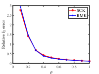
Simulation 1(a): changing . Set . For the Bernoulli distribution, the scaling parameter should be set within the range according to Example 1. Here, for simulation studies, we let range in .
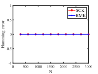
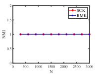
Simulation 1(b): changing . Let and range in .
The results are presented in Figure 1. We observe that SCK outperforms RMK because SCK returns more accurate estimations of and SCK runs faster than RMK across all settings. Both methods achieve better performances as increases, which conforms to our analysis in Example 1. Additionally, both algorithms enjoy better performances when the number of subjects increases, as predicted by our analysis following Corollary 1.


5.3.2 Binomial distribution
When for , we consider the following two simulations.
Simulation 2(a): changing . Set and . Recall that ’s range is when is Binomial distribution according to Example 2, here, we let range in .
Simulation 2(b): changing . Let , and range in .
Figure 2 presents the corresponding results. We note that SCK and RMK have similar error rates, while SCK runs faster than RMK for this simulation. Meanwhile, increasing (and ) decreases error rates for both methods, which confirms our findings in Example 2 and Corollary 1.


5.3.3 Poisson distribution
When for , we consider the following two simulations.
Simulation 3(a): changing . Set . Example 3 says that the theoretical range of is when is Poisson distribution. Here, we let range in .
Simulation 3(b): changing . Let and range in .
Figure 3 displays the numerical results of Simulation 3(a) and Simulation 3(b). The results are similar to those of the Bernoulli distribution case: SCK outperforms RMK in both estimating and running time; Both methods perform better as and increase, which supports our analysis in Example 3 and Corollary 1.


5.3.4 Normal distribution
When for , we consider the following two simulations.
Simulation 4(a): changing . Set and . According to Example 4, the scaling parameter can be set as any positive value when is Normal distribution. Here, we let range in .
Simulation 4(b): changing . Let , and range in .
Figure 4 shows the results. We see that SCK and RMK have similar performances in estimating model parameters while SCK runs faster than RMK. Additionally, the error rates of both approaches decrease when the scaling parameter and the number of subjects increase, supporting our findings in Example 4 and Corollary 1.


5.3.5 Exponential distribution
When for , we consider the following two simulations.
Simulation 5(a): changing . Set . According to Example 5, the range of the scaling parameter is when is Exponential distribution. Here, we let range in for our numerical studies.
Simulation 5(b): changing . Let and range in .
Figure 5 displays the results. We see that both methods provide satisfactory estimations for and for their small error rates, large NMI, and large ARI. SCK provides more accurate estimations than RMK and SCK takes less time for estimations than RMK. Meanwhile, we find that increasing does not significantly influence the performances of SCK and RMK and this verifies our theoretical analysis in Example 5 that disappears in the theoretical upper bounds of error rates by setting in Theorem 1 for Exponential distribution. Furthermore, when we increase , both methods perform better and this supports our analysis after Corollary 1.


5.3.6 Uniform distribution
When for , we consider the following two simulations.
Simulation 6(a): changing . Set . According to Example 6, the scaling parameter can be set as any positive value when is Uniform distribution. Here, we let range in .
Simulation 6(b): changing . Let and range in .
Figure 6 displays the numerical results. We see that increasing does not significantly decrease or increase estimation accuracies of SCK and RMK which verifies our theoretical analysis in Example 6. For all settings, SCK runs faster than RMK. When increasing , the Clustering error and Hamming error (NMI and ARI) for both approaches are 0 (1), and this suggests that SCK and RMK return the exact estimation of the classification matrix . This phenomenon occurs because is set quite large for Uniform distribution in Simulation 6(b). For the estimation of , error rates for both methods decrease when we increase and this is consistent with our findings following Corollary 1.


5.3.7 Signed response matrix
For signed response matrices when and for , we consider the following two simulations.
Simulation 7(a): changing . Set . Recall that the theoretical range of the scaling parameter is for signed response matrices according to our analysis in Example 7, here, we let range in .
Simulation 7(b): changing . Let and range in .
Figure 7 shows the results. We see that increasing and improves the estimation accuracies of SCK and RMK, which confirms our analysis in Example 7 and Corollary 1. Additionally, it is easy to see that both algorithms enjoy similar performances in estimating and , and SCK requires less computation time compared to RMK.


5.3.8 Simulated weighted response matrices
For visuality, we plot two weighted response matrices generated from the Normal distribution and the Poisson distribution under WLCM. Let for , and for . Because has been set, we can generate under different distributions with expectation under the proposed WLCM model. Here, we consider the following two settings.
Simulation 8 (a): When for , the left panel of Figure 8 displays a weighted response matrix generated from Simulation 8 (a).
Simulation 8 (b): When for , the right panel of Figure 8 provides a generated from Simulation 8 (b).
| Clustering error | Hamming error | NMI | ARI | Relative error | Relative error | |
| SCK | 0 (0) | 0 (0) | 1 (1) | 1 (1) | 0.0024 (0.0254) | 0.0032 (0.0295) |
| RMK | 0 (0) | 0 (0) | 1 (1) | 1 (1) | 0.0024 (0.0245) | 0.0032 (0.0295) |

Error rates of the proposed methods for the observed weighted response matrices provided in Figure 8 are displayed in Table 1. We also plot the estimated item matrix for both methods in Figure 9. We see that both approaches exactly recover from while they estimate with slight perturbations. Meanwhile, since and are known for this simulation, provided in Figure 8 can be regarded as benchmark weighted response matrices, and readers can apply SCK and RMK (and other methods) to to check their effectiveness in estimating and .
6 Real data applications
As the main goal of this paper is to introduce the proposed WLCM model and the SCK algorithm for weighted response matrices, this section reports empirical results on two data sets with weighted response matrices. Because the true classification matrix and the true item parameter matrix are unknown for real data, and SCK runs much faster than RMK, we only report the outcomes of the SCK approach. For real-world datasets, the number of extreme latent profiles is often unknown. Here, we infer for real-world weighted response matrices using the following strategy:
| (8) |
where and are outputs in Algorithm 2 with inputs and . The method specified in Equation (8) selects by picking the one that minimizes the spectral norm difference between and . The determination of the number of extreme latent profiles K in our WLCM model in a rigorous manner with theoretical guarantees remains a future direction.
6.1 International Personality Item Pool (IPIP) personality test data
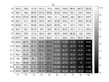
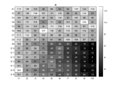
Background. We apply SCK to an experiment personality test data called the International Personality Item Pool (IPIP) personality test, which is obtainable for download at https://openpsychometrics.org/_rawdata/. This data consists of 1005 subjects and 40 items. The IPIP data also records the age and gender of each subject. After dropping subjects with missing entries in their responses, age, or gender, and dropping two subjects that are neither male nor female, there are 896 subjects left, i.e., . All items are rated on a 5-point scale, where 1=Strongly disagree, 2=Disagree, 3=Neither agree not disagree, 4=Agree, 5=Strongly agree, i.e., , a weighted response matrix. Items 1-10 measure the personality factor Assertiveness (short as “AS”); Items 11-20 measure the personality factor Social confidence (short as “SC”); Items 21-30 measure the personality factor Adventurousness (short as “AD”); Items 31-40 measure the personality factor Dominance (short as “DO”). The details of each item are depicted in Figure 10.
Analysis. We apply Equation (8) to infer for the IPIP dataset and find that the estimated value of is 3. We then apply the SCK algorithm to the response matrix with to obtain the matrix and the matrix . The running time for SCK on this dataset is around 0.2 seconds.
| profile 1 | profile 2 | profile 3 | |
| Size | 276 | 226 | 394 |
| #Male | 123 | 129 | 241 |
| #Female | 153 | 97 | 153 |
| Average age of male | 35.9837 | 32.8240 | 35.9004 |
| Average age of female | 35.5425 | 31.3814 | 38.7059 |
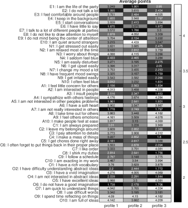
Results. For convenience, we denote the estimated three extreme latent profiles as profile 1, profile 2, and profile 3. Based on and the information of age and gender, we can obtain some basic information (shown in Table 2) such as the size of each profile, number of males (females) in each profile, and the average age of males (and females) in each profile. From Table 2, we see that the number of females is larger than that of males for profile 1 while profiles 2 and 3 have more males. The average age of males (and females) in profile 2 is smaller than that of profiles 1 and 3 while the average age of females in profile 3 is the largest. We can also obtain the average point on each item for males (and females) in each estimated extreme latent profile and the results are shown in panel (a) (and panel (b)) of Figure 10. We observe that males in profile 3 tend to be more confident, more creative, more social, and more open to changes than males in profiles 1 and 2; males in profile 3 are more (less) dominant than males in profile 1 (profile 2). Males in profile 2 are more confident&creative&social&open to changes&dominant than males in profile 1. Meanwhile, in the three estimated extreme latent profiles, females enjoy similar personalities to males. We also find that males in profile 3 (profile 2) are more (less) confident&creative&social&open to changes&dominant than females in profile 3 (profile 2). Furthermore, it is interesting to see that, though males in profile 1 are less confident&creative&social&open to changes than females in profile 1, they are more dominant than females in profile 1. We also plot the average point on each item in each estimated extreme latent profile regardless of gender in panel (c) of Figure 10 where we can draw similar conclusions as that for male. In panel (d) of Figure 10, we plot the heatmap of the estimated item parameter matrix . By comparing panel (c) with panel (d), we see that the -th element in the matrix shown in panel (c) is close to for . Such a result implies that the behavior differences on each item for every extreme latent profile are governed by the item parameter matrix .
Remark 5.
Recall that under the WLCM model, we have for . Then we have which gives that for . This interprets why the average value on the -th item in the -th estimated extreme latent profile approximates for .


6.2 Big Five Personality Test with Random Number (BFPTRN) data
Background. Our SCK method is also applied to personality test data: the Big Five Personality Test with Random Number (BFPTRN) data. This dataset can be downloaded from the same URL as the IPIP data. This data asks respondents to generate random numbers in certain ranges attached to 50 personality items. The Big Five personality traits are extraversion (items E1-E10), neuroticism (items N1-N10), agreeableness (items A1-A10), conscientiousness (items C1-C10), and openness (items O1-O10). The original BFPTRN data contains 1369 subjects. After excluding subjects with missing responses or missing random numbers and removing those with random numbers exceeding the specified range, there remain 1155 subjects, i.e., . All items are rated using the same 5-point scale as the IPIP data, which results in being weighted. The detail of each item and each range for random numbers can be found in Figure 11.
Analysis. The estimated number of extreme latent profiles for the BFPTRN dataset is 3. Applying the SCK approach to with produces the matrix and the matrix . SCK takes around 1.6 seconds to process this data.
Results. Without confusion, we also let profile 1, profile 2, and profile 3 represent the three estimated extreme latent profiles. Profile 1,2, and 3 have 409, 320, and 426 subjects, respectively. Similar to the IPIP data, based on and , we can also obtain the heatmap of the average point on each subject for every profile, the heatmap of the average random number on each range for every profile, and the heatmap of as shown in Figure 11. We observe that there is no significant connection between the average point and the average random number on each item in each estimated extreme latent profile. From panel (a) of Figure 11, we find that: for extraversion, subjects in profile 1 are the most extrovertive while subjects in profile 2 are the most introverted; for neuroticism, subjects in profile 3 are emotionally stable while subjects in profiles 1 and 2 are emotionally unstable; for agreeableness, subjects in profiles 1 and 3 are easier to get along with than subjects in profile 2; for conscientiousness, subjects in profile 3 are more responsible that those in profiles 1 and 2; for openness, subjects in profiles 1 and 3 are more open than those in profile 2. Meanwhile, the matrix shown in panel (a) approximates well, which has been explained in Remark 5.


7 Conclusion and future work
In this paper, we introduced the weighted latent class model (WLCM), a novel class of latent class analysis models for categorical data with weighted responses. We studied its model identifiability, developed an efficient inference method SCK to fit WLCM, and built a theoretical guarantee of estimation consistency for the proposed method under WLCM. On the methodology side, the new model WLCM provides exploratory and useful tools for latent class analysis in applications where the categorical data may have weighted responses. WLCM allows the observed weighted response matrix to be generated from any distribution as long as its expectation follows a latent class structure modeled by WLCM. In particular, the popular latent class model is a sub-model of our WLCM, and categorical data with signed responses can also be modeled by WLCM. Ground-truth latent classes of categorical data with weighted responses generated from WLCM serve as benchmarks for evaluating latent class analysis approaches. On the algorithmic side, the SVD-based spectral method SCK is efficient and easy to implement. SCK requires no tuning parameters and it is applicable for any categorical data with weighted responses. This means that researchers in fields such as social, psychological, behavioral, biological sciences, and beyond can design their tests/evaluations/surveys/interviews without worrying that the response should be binary or positive, as our method SCK is applicable for any weighted response matrices in latent class analysis. On the theoretic side, we established the rate of convergence for our method SCK under the proposed model WLCM. We found that SCK exhibits different behaviors when the weighted response matrices are generated from different distributions, and we conducted extensive experiments to verify our theoretical findings. Empirically, we applied our method to two real categorical datasets with weighted responses. We expect that our WLCM model and SCK method will have broad applications for latent class analysis of data with weighted responses in diverse fields, similar to the widespread use of latent class models in recent years.
There are several future directions worth exploring. First, methods with theoretical guarantees should be designed to determine the number of extreme latent profiles for observed weighted response matrices generated from any distribution under WLCM. Second, the grade of membership (GoM) model [44, 45] provides a richer modeling capacity than the latent class model since GoM allows a subject to belong to multiple extreme latent profiles. Therefore, following the distribution-free idea developed in this work, it is meaningful to extend the model GoM to categorical data with weighted responses. Third, like the LCM can be equipped with individual covariates [46, 47, 48, 49, 50, 51], it is worth considering additional individual covariates into the WLCM analysis. Fourth, our WLCM only considers static latent class analysis and it is meaningful to extend WLCM to the dynamic case [52]. Fifth, our SCK is a spectral clustering method and it is possible to speed up it by applications of the random-projection techniques [53] or the distributed spectral clustering idea [54] to deal with large-scale categorical data for latent class analysis.
CRediT authorship contribution statement
Huan Qing is the sole author of this paper.
Declaration of competing interest
The author declares no competing interests.
Data availability
Data and code will be made available on request.
Appendix A Proofs under WLCM
A.1 Proof of Proposition 1
Proof.
According to Lemma 1, we know that , where . Similarly, can be rewritten as , where . Then, for , we have
| (9) |
where denotes the extreme latent profile that the -th subject belongs in the alternative classification matrix . For and , we have
| (10) |
When , by the second statement of Lemma 1, we get . Combining this fact (i.e., ) with Equations (9) and (10) leads to
| (11) |
Equation (11) implies that when , i.e., for any two distinct subjects and , they are in the same extreme latent profile under when they are in the same extreme latent profile under . Therefore, we have , where is a permutation matrix. Combining with leads to , which gives that
| (12) |
Taking the transposition of Equation (12) gives
| (13) |
Right multiplying at both sides of Equation (14) gives
| (14) |
Since each extreme latent profile is not an empty set, the classification matrix has a rank , which gives that the matrix is nonsingular. Therefore, Right multiplying at both sides of Equation (14) gives , i.e., since is a permutation matrix. ∎
A.2 Proof of Lemma 1
Proof.
For the first statement: Since , , and the diagonal matrix is nonsingular, we have , where . Hence, the first statement holds.
For the second statement: For , gives . Then, if , we have , i.e., has distinct rows. Thus, the second statement holds.
For the third statement: Since , we have where the matrix is nonsingular because each extreme latent profile has at least one subject, i.e., . Thus, the third statement holds.
For the fourth statement: Recall that when , we have , is a full-rank diagonal matrix, and is a matrix, where . Let , then
| (15) |
It is straightforward to verify that is a column orthogonal matrix, i.e., .
Since , we have . Let be the compact SVD of , where is a diagonal matrix, , and . Note that and imply . Equation (15) implies
| (16) |
Note that , and are all orthonormal matrices. Also note that and are diagonal matrices. Then we have
| (17) |
Recall that , Equation (17) gives that and because and . We can easily verify that the rows of are perpendicular to each other and the -th row has length for , i.e., . Thus, the fourth statement holds.
Remark 6.
In this remark, we provide the reason why the fourth statement does not hold when . For this case, the rank of is , thus and . Then we have and . Thus, , which implies when and the fourth statement does not hold.
∎
A.3 Proof of Theorem 1
First, the following two lemmas are provided for our further proof.
Lemma 2.
Under , we have
where is a -by- orthogonal matrix.
Proof.
Lemma 3.
Under , if Assumption 1 is satisfied, then with probability at least ,
where is a positive constant.
Proof.
Proof.
Now, we prove the first statement of Theorem 1. Set as a small value, by Lemma 2 of [36] and the fourth statement of Lemma 1, if
| (19) |
then the Clustering error using the K-means algorithm. By setting , we see that Equation (19) always holds for all . So we get . According to Lemma 2, we have
By Lemma 3, we have
Next, we prove the second statement of Theorem 1. Since by Equation (3) in Lemma 1 and , we have which gives that and . We also have . Similarly, we have , where is the centroid matrix returned by K-means method for . Recall that , combine it with Equation (4) and Lemma 3, we have
Since is a matrix and in this paper, we have . Since holds for any matrix , we have . Thus, we have
| (20) |
Combing Equation (20) with the fact that gives
Recall that the -by- matrix satisfies , we have is at least of the order with high probability by applying the lower bound of the smallest singular value of a random rectangular matrix in [58]. Since in this paper, we have
∎
References
- [1] C. M. Dayton, G. B. Macready, Concomitant-variable latent-class models, Journal of the american statistical association 83 (401) (1988) 173–178.
- [2] J. A. Hagenaars, A. L. McCutcheon, Applied latent class analysis, Cambridge University Press, 2002.
- [3] J. Magidson, J. K. Vermunt, Latent class models, The Sage handbook of quantitative methodology for the social sciences (2004) 175–198.
- [4] G. Guo, J. Zhang, D. Thalmann, N. Yorke-Smith, Etaf: An extended trust antecedents framework for trust prediction, in: 2014 IEEE/ACM International Conference on Advances in Social Networks Analysis and Mining (ASONAM 2014), IEEE, 2014, pp. 540–547.
- [5] F. M. Harper, J. A. Konstan, The movielens datasets: History and context, Acm transactions on interactive intelligent systems (tiis) 5 (4) (2015) 1–19.
- [6] G. J. Meyer, S. E. Finn, L. D. Eyde, G. G. Kay, K. L. Moreland, R. R. Dies, E. J. Eisman, T. W. Kubiszyn, G. M. Reed, Psychological testing and psychological assessment: A review of evidence and issues., American psychologist 56 (2) (2001) 128.
- [7] J. J. Silverman, M. Galanter, M. Jackson-Triche, D. G. Jacobs, J. W. Lomax, M. B. Riba, L. D. Tong, K. E. Watkins, L. J. Fochtmann, R. S. Rhoads, et al., The american psychiatric association practice guidelines for the psychiatric evaluation of adults, American Journal of Psychiatry 172 (8) (2015) 798–802.
- [8] J. De La Torre, L. A. van der Ark, G. Rossi, Analysis of clinical data from a cognitive diagnosis modeling framework, Measurement and Evaluation in Counseling and Development 51 (4) (2018) 281–296.
- [9] Y. Chen, X. Li, S. Zhang, Joint maximum likelihood estimation for high-dimensional exploratory item factor analysis, Psychometrika 84 (2019) 124–146.
- [10] Z. Shang, E. A. Erosheva, G. Xu, Partial-mastery cognitive diagnosis models, The Annals of Applied Statistics 15 (3) (2021) 1529–1555.
- [11] K. T. Poole, Nonparametric unfolding of binary choice data, Political Analysis 8 (3) (2000) 211–237.
- [12] J. Clinton, S. Jackman, D. Rivers, The statistical analysis of roll call data, American Political Science Review 98 (2) (2004) 355–370.
- [13] R. Bakker, K. T. Poole, Bayesian metric multidimensional scaling, Political analysis 21 (1) (2013) 125–140.
- [14] Y. Chen, Z. Ying, H. Zhang, Unfolding-model-based visualization: theory, method and applications, The Journal of Machine Learning Research 22 (1) (2021) 548–598.
- [15] J. Martinez-Moya, M. Feo-Valero, Do shippers’ characteristics influence port choice criteria? capturing heterogeneity by using latent class models, Transport Policy 116 (2022) 96–105.
- [16] A. K. Formann, T. Kohlmann, Latent class analysis in medical research, Statistical methods in medical research 5 (2) (1996) 179–211.
- [17] A. Kongsted, A. M. Nielsen, Latent class analysis in health research, Journal of physiotherapy 63 (1) (2017) 55–58.
- [18] Z. Wu, M. Deloria-Knoll, S. L. Zeger, Nested partially latent class models for dependent binary data; estimating disease etiology, Biostatistics 18 (2) (2017) 200–213.
- [19] P. G. Van der Heijden, J. Dessens, U. Bockenholt, Estimating the concomitant-variable latent-class model with the em algorithm, Journal of Educational and Behavioral Statistics 21 (3) (1996) 215–229.
- [20] Z. Bakk, J. K. Vermunt, Robustness of stepwise latent class modeling with continuous distal outcomes, Structural equation modeling: a multidisciplinary journal 23 (1) (2016) 20–31.
- [21] H. Chen, L. Han, A. Lim, Beyond the em algorithm: constrained optimization methods for latent class model, Communications in Statistics-Simulation and Computation 51 (9) (2022) 5222–5244.
- [22] Y. Gu, G. Xu, A joint mle approach to large-scale structured latent attribute analysis, Journal of the American Statistical Association 118 (541) (2023) 746–760.
- [23] A. Anandkumar, R. Ge, D. Hsu, S. M. Kakade, M. Telgarsky, Tensor decompositions for learning latent variable models, Journal of machine learning research 15 (2014) 2773–2832.
- [24] Z. Zeng, Y. Gu, G. Xu, A tensor-em method for large-scale latent class analysis with binary responses, Psychometrika 88 (2) (2023) 580–612.
- [25] A. K. Formann, Constrained latent class models: Theory and applications, British Journal of Mathematical and Statistical Psychology 38 (1) (1985) 87–111.
- [26] B. Lindsay, C. C. Clogg, J. Grego, Semiparametric estimation in the rasch model and related exponential response models, including a simple latent class model for item analysis, Journal of the American Statistical Association 86 (413) (1991) 96–107.
- [27] N. L. Zhang, Hierarchical latent class models for cluster analysis, The Journal of Machine Learning Research 5 (2004) 697–723.
- [28] C.-C. Yang, Evaluating latent class analysis models in qualitative phenotype identification, Computational statistics & data analysis 50 (4) (2006) 1090–1104.
- [29] G. Xu, Identifiability of restricted latent class models with binary responses, The Annals of Statistics 45 (2) (2017) 675 – 707.
- [30] G. Xu, Z. Shang, Identifying latent structures in restricted latent class models, Journal of the American Statistical Association 113 (523) (2018) 1284–1295.
- [31] W. Ma, W. Guo, Cognitive diagnosis models for multiple strategies, British Journal of Mathematical and Statistical Psychology 72 (2) (2019) 370–392.
- [32] Y. Gu, G. Xu, Partial identifiability of restricted latent class models, The Annals of Statistics 48 (4) (2020) 2082 – 2107.
- [33] M. E. Newman, Analysis of weighted networks, Physical review E 70 (5) (2004) 056131.
- [34] T. Derr, C. Johnson, Y. Chang, J. Tang, Balance in signed bipartite networks, in: Proceedings of the 28th ACM International Conference on Information and Knowledge Management, 2019, pp. 1221–1230.
- [35] K. Goldberg, T. Roeder, D. Gupta, C. Perkins, Eigentaste: A constant time collaborative filtering algorithm, information retrieval 4 (2001) 133–151.
- [36] A. Joseph, B. Yu, Impact of regularization on spectral clustering, Annals of Statistics 44 (4) (2016) 1765–1791.
- [37] J. Jin, Fast community detection by SCORE, Annals of Statistics 43 (1) (2015) 57–89.
- [38] A. Strehl, J. Ghosh, Cluster ensembles—a knowledge reuse framework for combining multiple partitions, Journal of machine learning research 3 (Dec) (2002) 583–617.
- [39] L. Danon, A. Diaz-Guilera, J. Duch, A. Arenas, Comparing community structure identification, Journal of statistical mechanics: Theory and experiment 2005 (09) (2005) P09008.
- [40] J. P. Bagrow, Evaluating local community methods in networks, Journal of Statistical Mechanics: Theory and Experiment 2008 (05) (2008) P05001.
- [41] W. Luo, Z. Yan, C. Bu, D. Zhang, Community detection by fuzzy relations, IEEE Transactions on Emerging Topics in Computing 8 (2) (2017) 478–492.
- [42] L. Hubert, P. Arabie, Comparing partitions, Journal of classification 2 (1985) 193–218.
- [43] N. X. Vinh, J. Epps, J. Bailey, Information theoretic measures for clusterings comparison: is a correction for chance necessary?, in: Proceedings of the 26th annual international conference on machine learning, 2009, pp. 1073–1080.
- [44] M. A. Woodbury, J. Clive, A. Garson Jr, Mathematical typology: a grade of membership technique for obtaining disease definition, Computers and biomedical research 11 (3) (1978) 277–298.
- [45] E. A. Erosheva, Comparing latent structures of the grade of membership, rasch, and latent class models, Psychometrika 70 (4) (2005) 619–628.
- [46] G.-H. Huang, K. Bandeen-Roche, Building an identifiable latent class model with covariate effects on underlying and measured variables, Psychometrika 69 (1) (2004) 5–32.
- [47] A. Forcina, Identifiability of extended latent class models with individual covariates, Computational Statistics & Data Analysis 52 (12) (2008) 5263–5268.
- [48] B. A. Reboussin, E. H. Ip, M. Wolfson, Locally dependent latent class models with covariates: an application to under-age drinking in the usa, Journal of the Royal Statistical Society Series A: Statistics in Society 171 (4) (2008) 877–897.
- [49] J. K. Vermunt, Latent class modeling with covariates: Two improved three-step approaches, Political analysis 18 (4) (2010) 450–469.
- [50] R. Di Mari, Z. Bakk, A. Punzo, A random-covariate approach for distal outcome prediction with latent class analysis, Structural Equation Modeling: A Multidisciplinary Journal 27 (3) (2020) 351–368.
- [51] Z. Bakk, R. Di Mari, J. Oser, J. Kuha, Two-stage multilevel latent class analysis with covariates in the presence of direct effects, Structural Equation Modeling: A Multidisciplinary Journal 29 (2) (2022) 267–277.
- [52] T. Asparouhov, E. L. Hamaker, B. Muthén, Dynamic latent class analysis, Structural Equation Modeling: A Multidisciplinary Journal 24 (2) (2017) 257–269.
- [53] H. Zhang, X. Guo, X. Chang, Randomized spectral clustering in large-scale stochastic block models, Journal of Computational and Graphical Statistics 31 (3) (2022) 887–906.
- [54] S. Wu, Z. Li, X. Zhu, A distributed community detection algorithm for large scale networks under stochastic block models, Computational Statistics & Data Analysis (2023) 107794.
- [55] Z. Zhou, A. A. Amini, Analysis of spectral clustering algorithms for community detection: the general bipartite setting, Journal of Machine Learning Research 20 (47) (2019) 1–47.
- [56] H. Qing, J. Wang, Community detection for weighted bipartite networks, Knowledge-Based Systems 274 (2023) 110643.
- [57] J. A. Tropp, User-friendly tail bounds for sums of random matrices, Foundations of Computational Mathematics 12 (4) (2012) 389–434.
- [58] M. Rudelson, R. Vershynin, Smallest singular value of a random rectangular matrix, Communications on Pure and Applied Mathematics: A Journal Issued by the Courant Institute of Mathematical Sciences 62 (12) (2009) 1707–1739.