LaSDI: Parametric Latent Space Dynamics Identification
Abstract
Enabling fast and accurate physical simulations with data has become an important area of computational physics to aid in inverse problems, design-optimization, uncertainty quantification, and other various decision-making applications. This paper presents a data-driven framework for parametric latent space dynamics identification procedure that enables fast and accurate simulations. The parametric model is achieved by building a set of local latent space model and designing an interaction among them. An individual local latent space dynamics model achieves accurate solution in a trust region. By letting the set of trust region to cover the whole parameter space, our model shows an increase in accuracy with an increase in training data. We introduce two different types of interaction mechanisms, i.e., point-wise and region-based approach. Both linear and nonlinear data compression techniques are used. We illustrate the framework of Latent Space Dynamics Identification (LaSDI) enable a fast and accurate solution process on various partial differential equations, i.e., Burgers’ equations, radial advection problem, and nonlinear heat conduction problem, achieving x speed-up and relative error with respect to the corresponding full order models.
1 Introduction
Physical simulations have influenced developments in engineering, technology, and science more rapidly than ever before. The widespread application of simulations as digital twins is one recent example. Advances in optimization and control theory have also increased simulation predictability and practicality. Physical simulations can reproduce responses in a variety of systems, from quantum mechanics to astrophysics, with considerable detail and accuracy, and they provide information that often cannot be obtained from experiments or in-situ measurements due to associated high risks and measurement difficulties. However, high-fidelity forward physical simulations are computationally expensive and, thus, make intractable any decision-making applications, such as inverse problems, design optimization, optimal controls, uncertainty quantification, and parameter studies, where many forward simulations are required.
To compensate for the computational expense issue, researchers develop several surrogate models to accelerate the physical simulations with high accuracy. One particular type is projection-based reduced order model (pROM), in which the full state fields are approximated by applying linear or nonlinear compression techniques. A popular linear compression technique include proper orthogonal decomposition (POD) [1], reduced basis method [2], and balanced truncation method [3], while a popular nonlinear compression technique is auto-encoder (AE) [4, 5, 6, 7]. The linear compression-based pROM is successfully applied to many different problems, such as Lagrangian hydrodynamics [8, 9], Burgers equations [10, 11, 12], nonlinear heat conduction problem [13], aero-elastic wing design problem [14], Navier–Stokes equation [15], computational fluid dynamics simulation for aircraft [16], convection–diffusion equation [17], Boltzman transport problem [18], topology optimization [19], the shape optimization of a simplified nozzle inlet model and the design optimization of a chemical reaction [20], and lattice-type structure design [21]. These projection-based ROMs are further categorized by its intrusiveness. The intrusive ROMs plug the reduced solution representation into the underlying physics law, governing equations, and its numerical discretization methods, such as the finite element, finite volume, and finite difference methods. Therefore, they are physics-constrained data-driven approaches and require less data than the methods that only require data to achieve the same level of accuracy. However, one needs to understand the underlying numerical methods of solving the high-fidelity simulation to implement the intrusive ROMs. Furthermore, the intrusive ROMs are only applicable when the source code for a high-fidelity physics solver is available, which is not the case for certain applications. On the other hand, the non-intrusive ROMs do not require the access to the source code of a high-fidelity physics solver. Therefore, we will focus on developing the non-intrusive ROMs, which use only data to approximate the full state fields.
Among many non-intrusive methods, various interpolation techniques are used to build a nonlinear map that predicts new outputs for new inputs. The interpolation techniques include, but not limited to, Gaussian processes [22, 23], radial basis functions [24, 25], Kriging [26, 27], and convolutional neural networks [28, 29]. Among them, neural networks have been the most popular framework because of their rich representation capability supported by the universal approximation theorem. Such surrogate models have been applied to various physical simulations, including, but not limited to, particle simulation [30], nanophotonic particle design [31], porous media flow [32, 33, 34, 35], storm prediction [36], fluid dynamics [37], hydrology [38, 39], bioinformatics [40], high-energy physics [41], turbulence modeling [42, 43, 44, 45], uncertainty propagation in a stochastic elliptic partial differential equation [46], bioreactor with unknown reaction rate [47], barotropic climate models [48], and deep Koopman dynamical models [49]. These methods have the potential to be extended to experimental video data as done in [50], where intrinsic dimension is sought through auto-encoder training. However, these methods lack the interpretability due to the black-box nature caused by its complex underlying structure of interpolators, e.g., neural networks. Furthermore, they do not aim to predict the state field solution in general. Therefore, if the target output quantity of interest changes, the model needs to go through the expensive training phase again, which shows the lack of generalizability.
To improve the interpretability and generalizability, we focus on developing a latent space dynamics learning algorithm, where the whole state field data is compressed into a reduced space and the dynamics in the reduced space is learned. Two different types of compression are possible, i.e., linear and nonlinear compression. The popular linear compression can be realized by the singular value decomposition (SVD), justified by the proper orthogonal decomposition (POD) framework. The popular nonlinear compression can be accomplished by the auto-encoder (AE), where the encoder and decoder are designed with neural networks. After the compression, the data size is reduced tremendously. Moreover, the dynamics of the data within the reduced space is often much simpler than the dynamics of the full space. For example, Figure 1 shows the reduced space dynamics corresponding to 2D radial advection problems. This motivates our current work to identify the simplified and reduced but latent dynamics with a system identification regression technique.

There are many existing latent space learning algorithms. DeepFluids [51] uses the auto-encoder for nonlinear compression and applies the latent space time integrator to propagate the solution in the reduced space. The authors in [34] and [52] use both linear and nonlinear compressions and apply some interpolation techniques, such as artificial neural networks (ANNs) and radial basis function (RBF) interpolations within the reduced space to predict the solution for new parameter value. Xie, et al., in [53] uses POD as linear compression technique and apply linear multi-step neural network to predict and propagate the latent space dynamical solutions. Hoang, et al., in [54] compresses both space and time solution space with POD, which was first introduced in [11]. Then they use several interpolation techniques, such as polynomial regression, -nearest neighbor regression, random forest regression, and neural network regression, within the reduced space formed by the space–time POD. However, all the aforementioned methods use a complex form as a latent space dynamics model, whose structure is not well understood and lacking the interpretability. On the other hand, Champion, et al., in [55] use an auto-encoder for the compression and the sparse identification of nonlinear dynamics (SINDy) to identify ordinary differential equations (ODEs) for the latent space dynamics, which is simpler than neural networks, improving the interpretability. However, they fail to generalize the method to achieve a robust parametric model. It is partly because one system of ODEs is not enough to cover all the variations within the latent space due to parameter change.
Therefore, we propose to identify latent space dynamics with a set of local system of ODEs that is tailored to improve the accuracy on a local area of the parameter space. This implies that each local model has a trust region, which covers a sub-region of the whole parameter space. If the set of the trust region covers the whole parameter space, then our model is guaranteed to achieve a certain accuracy level everywhere, achieving truly parametric model based on latent space learning algorithm. At the same time, the framework enables a faster calculation than the corresponding high-fidelity model. We call this framework, LaSDI, which stands for Latent Space Dynamics Identification.
The procedure of LaSDI is summarized by four distinct steps below and its schematics are depicted in Figure 2:
-
1.
Data Generation: Generate full order model (FOM) simulation data, i.e., parametric time dependent solution data
-
2.
Compression: Apply compression on the simulation data, through either singular value decomposition or auto-encoder to form latent space data.
-
3.
Dynamics Identification: Identify the governing equations that best matches the latent space data in a least-squares sense.
-
4.
Prediction: Use the identified governing equation to predict the latent space solution for a new parameter point. In this paper, we assume that the parameter affects only the initial condition. The predicted latent space solution is reconstructed to the full state by decompression.

In fact, the four-step procedure above is prevalent in developing data-driven reduced-order models to accelerate physical simulations. The traditional data-driven projection-based reduced order models mentioned earlier follow the four-step procedure if the dynamics identification model is derived from the existing physical governing equations. The dynamic mode decomposition (DMD) approaches [56, 57, 58, 59, 60, 61, 62, 63, 64, 65, 66, 67, 68, 69] also follow the four-step procedure, where linear compression via SVD is used for Step 2 and linear ODEs are generally used for Step 3. Additionally, the operator inference (OpInf) approaches [70, 71, 72, 73, 74, 75, 76, 77, 78, 79, 80, 81, 82], which utilize linear compression and fit the latent space dynamics data into polynomial models (mostly quadratic models), also follow the four-step procedure above. As a matter of fact, the proposed LaSDI in this paper is similar to both DMD and OpInf approaches. The major two differences include (i) in Step 2, LaSDI allows for nonlinear compression via an auto-encoder, while DMD and OpInf use a linear compression via the SVD; and (ii) in Step 3, DMD and OpInf only considers polynomial terms in the candidate library, while LaSDI allows general nonlinear terms. Therefore, LaSDI can be viewed as a generalization of both DMD and OpInf.
The main contributions of this paper include
-
•
A generalized data-driven physical simulation framework, i.e., LaSDI, is introduced.
-
•
A novel local latent space learning algorithm that demonstrates robust parametric prediction, is introduced.
-
•
Three novel dynamics identification algorithms are introduced, i.e., global, local, and interpolated ones.
-
•
Both good accuracy and speed-up are demonstrated with several numerical experiments.
The paper is organized in the following way: Section 3 technically describes LaSDI, where each four distinct steps are explained in details. Section 3.1 describes how to generate and store the simulation data. Section 3.2 discusses two different types of compression techniques. Section 3.3 elaborates the procedure of the dynamics identification and subsequently describes three different types. Section 3.4 elucidates the prediction step. We demonstrate the performance of LaSDIs for four different numerical experiments in Section 4, where global, local, and interpolated dynamics identification algorithms are compared and analyzed. Finally, we summarize and discuss the implications, limitations, and potential future directions for LaSDI in Section 5.
2 Dynamical system of equations
We formally state a parameterized dynamical system, characterized by the following time dependent ordinary differential equations (ODEs):
| (1) |
where denotes time with the final time , and denotes the time-dependent, parameterized state implicitly defined as the solution to System (1) with . Further, with denotes the scaled velocity of , which can be either linear or nonlinear in its first argument. The initial state is denoted by , and denotes the parameters with parameter domain . We assume that the parameter affects only the initial condition. System (1) can be considered as semi-discretized version of a system of partial differential equations (PDEs), whose spatial domain is denoted as , , where . The spatial discretization can be done through many different numerical methods, such as the finite difference, finite element, and finite volume methods.
Many different time integrators are available to approximate the time derivative term, , e.g., explicit and implicit time integrators. A uniform time discretization is assumed throughout the paper, characterized by time step and time instances for with , . To avoid notational clutter, we introduce the following time discretization-related notations: , , , and .
Although many advanced numerical methods are available to solve System (1), as the problem size increases, i.e., a large , and the computational domain gets geometrically complicated, the overall solution time becomes impractically slow, e.g., taking a day or week for one forward simulation. The proposed method, i.e., LaSDI, accelerates the computationally expensive simulations.
3 LaSDI
This section mathematically describes LaSDI. As shown in Introduction 1, LaSDI consists of four steps, i.e., data generation, compression, identification, and prediction. Each step is described in the subsequent sections.
3.1 Data generation
LaSDI first generates full order model simulation data by solving a system of dynamical system (1) by sampling parameter space, . We denote the sampling points by , where denotes a training set. We also denote for the -th time step solution of (1) with and arrange the snapshot matrix for . Concatenating all the snapshot matrices side by side, the whole snapshot matrix is defined as
| (2) |
3.2 Compression
The second step of LaSDI is to compress the snapshot matrix either using linear or nonlinear compression techniques. The choice of either linear or nonlinear compression can be determined by the Kolmogorov -width, which quantifies the optimal linear subspace. It is defined as:
| (3) |
where denotes the manifold of solutions over all time and parameters and denotes all -dimensional subspace. If a problem has a solution space whose Kolmogorov -width decaying fast, then the the linear compression will provide an efficient subspace that can accurately approximates a true solution. However, a problem has a solution space with Kolmogorov -width decaying slowly, then the linear compression will not be sufficient for good accuracy. Then, the nonlinear compression is necessary. The rate of decay in Kolmogorov -width can be well indicated by the singular value decay (see Figure 3). Section 3.2.1 describes a linear compression technique, i.e., proper orthogonal decomposition, which leads to LaSDI-LS where LS stands for “Linear Subspace.” Section 3.2.2 describes a nonlinear compression technique, i.e., auto-encoder, which leads to LaSDI-NM where NM stands for “Nonlinear Manifold.”
3.2.1 Proper orthogonal decomposition: LaSDI-LS
We follow the method of snapshots first introduced by Sirovich [83]. The spatial basis from POD is an optimally compressed representation of in a sense that it minimizes the projection error, i.e., the difference between the original snapshot matrix and the projected one onto the subspace spanned by the basis, :
| (4) |
where denotes the Frobenius norm. The solution of POD can be obtained by setting , , where is th column vector of the left singular matrix, , of the following Singular Value Decomposition (SVD),
| (5) |
Once the basis is built, the snapshot matrix can be reduced to the generalized coordinate matrix, , so called, the reduced snapshot matrix in the subspace spanned by column vectors of , i.e.,
| (6) |
Naturally, we can define the reduced snapshot matrix, , tailored for by extracting from th to th column vectors of , i.e.,
| (7) |
where is the reduced coordinates at th time step for . The matrix describes the latent space trajectory corresponding to . For example, Step 2 of Figure 2 shows a graph of the latent space trajectory for the last parameter value, . These reduced coordinates data will be used to train either global or local DI models to identify the dynamics of the latent space (see Section 3.3).

3.2.2 Auto-encoder: LaSDI-NM
Auto-encoders act as a nonlinear analogue to POD. As illustrated in [4], nonlinear subspace generated by auto-encoders outperform those generated by POD. In general, we train two neural networks, and to minimize
| (8) |
where MSE denotes the mean-squared error. As above, we can define
| (9) |
and can extract the snapshot by considering the th to th columns of .
The general architecture of and may vary. For the purposes of this paper, we will use a masked-shallow network as described in [4]. The use of this network architecture allows for universality across various PDEs and data shapes. The masking of the network allows for increased efficiency by not including full linear layers. However, the masking requires that we take care when constructing neural networks for higher dimensional simulations because the organization of spatial data must match the masking. Specifically, the architecture of both and consists of three layers, i.e., input, output and one hidden layer. The first layers are fully connected with nonlinear activation functions, whereas the final layer does not have nonlinear activation functions, i.e., fully linear. Then, the a masking operator is applied to make sparse. We make the sparsity of the mask matrix similar to the one in the mass matrix to respect the sparsity induced by the underlying numerical scheme. Further details on the architecture of the neural networks can be found in [4].
When training the auto-encoder, becomes a key hyper-parameter. Similar to POD, if is too small, the compression-decompression technique incurs a significant loss of data. Thus, cannot be chosen too small. In contrast to the POD, where increasing the basis size, improves results, this is not always the case with an auto-encoder. Rather, for larger , significant improvement the error might not be seen. Further, when applying the DI techniques as described below, high-dimensional complex nonlinear systems are harder to approximate than those with simpler dynamics. Thus, we tune to be the smallest possible dimension while not compromising the accuracy of the reconstructed snapshot matrix.
3.3 Dynamics Identification
To identify the latent space dynamics, we employ regression methods inspired by SINDy [84]. SINDy uses sparse regression tools, such as a sequential threshold least-squares, Lasso, Ridge, and Elastic Net. However, we do not require that our discovered dynamical system to be sparse in LaSDI. Instead, we want to generate the dynamical system that, when integrated, generates the most numerically accurate results. Because we do not require our solution to be sparse, we will refer this identification step to dynamics identification (DI).
In general, we aim to find a dynamical system whose discrete solution best-matches the latent space discrete trajectory data, in a least-squares sense. The goal is to identify a good . To formally describe the DI procedure, we take the transpose of the latent space trajectory data, i.e., , to arrange the temporal evolution in a downward direction:
| (10) |
Then we approximate the time derivative term with a finite difference and arrange the temporal evolution in a downward direction as well:
| (11) |
We prescribe a library of functions, i.e., , to approximate the right-hand side of the dynamical system, i.e., . For example, may take a form of constant, polynomial, trigonometric, and exponential functions:
| (12) |
where denotes the number of columns, which is determined by the choice of a library of functions, and represents all the polynomials with order . For the numerical examples in this paper, are sufficient for accurate approximation of the dynamical system. For example, and are defined as
| (13) |
and
| (14) |
The introduction of , , and in Eqs. (10), (11), and (12) allows us to write the following regression problem:
| (15) |
So far, we have shown how to build local DI for a specific sample parameter, i.e., . However, this is not the only option. As a matter of fact, one can build a DI model for multiple parameter values. This observation leads to two types of DI: one, using all the training data to inform the underlying dynamical system; two, using only training data close to a query parameter point to model the dynamics. The former we refer to as Global DI and the latter, Local DI. Note that both global and Local DIs can be considered as region-based because they set a unified DI for each region. Alternatively, we can consider point-wise DIs, where the coefficients, of each DI model built for a single training point, i.e., , by Eq. (15) can be interpolated for a new query point, . We refer the detailed explanation of such interpolation to interpolated DI.
3.3.1 Region-based global DI
Global DI requires a straight-forward implementation. We include all the training snapshots in the identification of the latent space dynamics. For this, the discovered dynamics come from modifying (15) to
| (16) |
This gives one universal DI model that covers the whole parameter space, which might be a good model if the latent space dynamics do not drastically change based on parameter values. This might be valid for a small parameter space. However, for a larger parameter space, the latent space dynamics might change drastically. Therefore, we introduce local DI.
3.3.2 Region-based local DI
For a large parameter space, we should not expect that a single dynamical system would govern all the latent space trajectories from the whole training data. However, we might expect that the dynamics in the latent space locally behave. This observation allows us to build a local DI which provides a good model for a local region. The local DI takes training simulation data from neighboring points. Therefore, the least-squares regression problem for th local DI becomes
| (17) |
where denotes a set of training parameters that determine th local parameter region and its corresponding set of indices is denoted as . The th local parameter region, , is defined by the set of points that are closest to parameters in with some distance measure, i.e.,
| (18) |
where denotes a distance between two points in . We use Euclidean distance that is defined as
| (19) |
but other distance functions can be used as well. Note that is a parameter that can be tuned. If , we recover the global DI. Therefore, the global DI can be considered as a special case of local DIs. We illustrate the various examples of global and local DI in a 2D parameter space and their local parameter region which are relevant to a specific denoted as pink dots in Figure 4.

3.3.3 Point-wise interpolated DI
For , the interpolated DI interpolates coefficients, , for if , where are obtained by solving Eq. (15), to obtain the interpolated coefficients, , which will be used for the LaSDI prediction in Eq. (23). Many interpolation techniques can be utilized here, but we use two techniques: radial basis functions (RBFs) and linear bi-variate splines. In each case, we interpolate element-wise in . For the elements in , the corresponding interpolation functions are defined below.
The RBF interpolation function for each element of for , is defined as
| (20) |
where are radial basis functions; denotes th RBF interpolation coefficient, which is obtained by solving a least-squares problem; is the Euclidean distance as defined in Eq. (19); and . Many radial basis functions are available. For our numerical experiments, we use the multiquadric radial basis functions defined as
| (21) |
where approximates average distance between .
The linear bi-variate splines approximates using a linear combination of the based on with no smoothing. If falls on a uniform grid, as in our numerical experiments, the bi-linear interpolation function for each entry of can be defined in rectangular regions. For example, in two dimensional parameter space, this is defined by the four corner points in a specific region (e.g., ), , , , and the corresponding s. For , each entry of can be obtained by
| (22) |
3.3.4 Notes on DIs
In general, finding an accurate and numerically stable approximation can be difficult for unknown nonlinear problems. Because of this, the terms included in the regression becomes a hyper-parameter that must be tuned. As with tuning , we strive to use the least number of terms for best accuracy. Therefore, we now discuss the procedure used to obtain the best dynamics approximation given a set of trajectories in a latent space:
-
1.
Start simple: start with polynomial order one. This generates the linear dynamical system that best approximates the latent space dynamics.
-
2.
Verification: Visually verify that the new trajectories approximate the training data.
-
3.
If a better fit is required, we include the following modifications in order of importance:
-
•
Rescale: rescale the data so that .
-
•
Enrich: enrich the library with more terms, such as polynomials with a higher order, mixed polynomial terms (e.g., ), trigonometric and exponential terms.
-
•
Solving one of the least-squares problems, i.e., Eqs. (15), (16), and (17), or utilizing point-wise approach in Section 3.3.3 gives a latent space dynamical system characterized by the form of a system of ordinary differential equations (ODEs):
| (23) |
where right-hand-side, , is determined by a library of functions specified in Eq. (12) and the coefficients identified from the least-squares problems or interpolations.
3.4 Prediction
After local or global or interpolated DIs are set in the dynamics identification step, one can solve them to predict new latent space dynamics trajectories corresponding to a new parameter . If the global DI is used, there is no ambiguity. However, if a local DIs are used, then one needs to figure out which local DI needs to be solved. It can be determined by checking . However, pre-defining over the whole parameter space, , can be a daunting process for non-uniform training points. Therefore, the interpolated DIs might be more practical for non-uniform training points.
3.4.1 Latent space dynamics solve and reconstruction
Once an appropriate DI is recognized for a given , an appropriate initial condition is required. The latent space initial condition corresponding to is obtained by applying compression step to the full order model initial condition corresponding to as described in Section 3.2. For the linear compression,
| (24) |
and for the nonlinear compression,
| (25) |
are used. Using this initial condition, Eq. (23) is solved to predict the latent space dynamics trajectory, using the Dormand-Prince pair of formulas [85]. At each iteration, the local error is controlled using a fourth-order method. Using local extrapolation, the step is then taken using a fifth-order formulation. Then, the approximated full state trajectories, are restored by if the linear compression were used and by if the autoencoder is used as a nonlinear compression.
4 Numerical Results
We demonstrate the performance of LaSDI for four different numerical examples, i.e., 1D and 2D Burgers equations, heat conduction, and radial advection problems. The governing equations, initial conditions, boundary conditions, parameter space, and domain are specified in Table 1.
| Equation | Initial Condition | Domain/Boundary | ||||
|---|---|---|---|---|---|---|
|
||||||
|
||||||
|
||||||
|
For both 1D and 2D Burgers problems, a uniform space discretization (i.e., for 1D and for 2D Burgers problems) is used for the full order model solve. The first order spatial derivative term is approximated by the backward difference scheme, while the diffusion terms are approximated by the central difference scheme. This generates a semi-discretized PDE characterized by a system of nonlinear ordinary differential equations specified in Eq. (1). We integrate each of these systems over a uniform time-step (i.e., for 1D and for 2D Burgers problems) using the implicit backward Euler time integrator, i.e., .
For the full order model of the nonlinear heat conduction problem, we use the second order finite element to discretize the spatial domain. The spatial discretization starts with uniform squares, which are divided into triangular elements, resulting in 8192 triangular elements in total. A uniform time step of is used with the SDIRK3 implicit L-stable time integrator (i.e., see Eq. (229) of [87]). For the temperature field dependent conductivity coefficient, we linearize the problem by using the temperature field from the previous time step.111The source code of the full order model for the nonlinear heat conduction problem can be found at https://github.com/mfem/mfem/blob/master/examples/ex16.cpp
For the full order model of the radial advection problem, we use the third order discontinuous finite element to discretize the spatial domain. The spatial discretization is dictated by a square-mesh with periodic boundary conditions. We use grid of square finite elements. The finite element data is interpolated to generate a uniform grid across the spatial domain. We use a uniform time step of with the RK4 explicit time integrator.222The source code of the full order model for the radial advection problem can be found at https://github.com/mfem/mfem/blob/master/examples/ex9.cpp
These full order models are used to generate training data. Table 2 shows testing parameter set, , as well as all the training samples, , for four problems. Note that the testing points include the training points. The accuracy is measured by the maximum relative error, , at each testing parameter point, which is defined as
| (26) |
where is a testing parameter point.
| Example | Training set, | Testing set, |
|---|---|---|
| 1D Burgers | ||
| 2D Burgers | ||
| Heat Conduction | ||
| Radial Advection |
The computational cost is measured in terms of the wallclock time. Specifically, timing is obtained by performing calculations on a IBM Power9 @ 3.50 GHz and DDR4 Memory @ 1866 MT/s. The auto-encoders are trained on a NVIDIA V100 (Volta) GPU with 3168 NVIDIA CUDA Cores and 64 GB GDDR5 GPU Memory using PyTorch [55] which is the open source machine learning frame work.
4.1 1D Burgers
First, for both LaSDI-LS and LaSDI-NM, we approximate the dynamics with linear dynamical systems in global DI. In Figure 5, the last time step solutions for are compared with the corresponding FOM solution, showing that they are almost identical. This shows that LaSDIs are able to accurately predict solutions. Figure 6 illustrates the relative error of a LaSDI model is bounded below by the projection error of the compression technique.


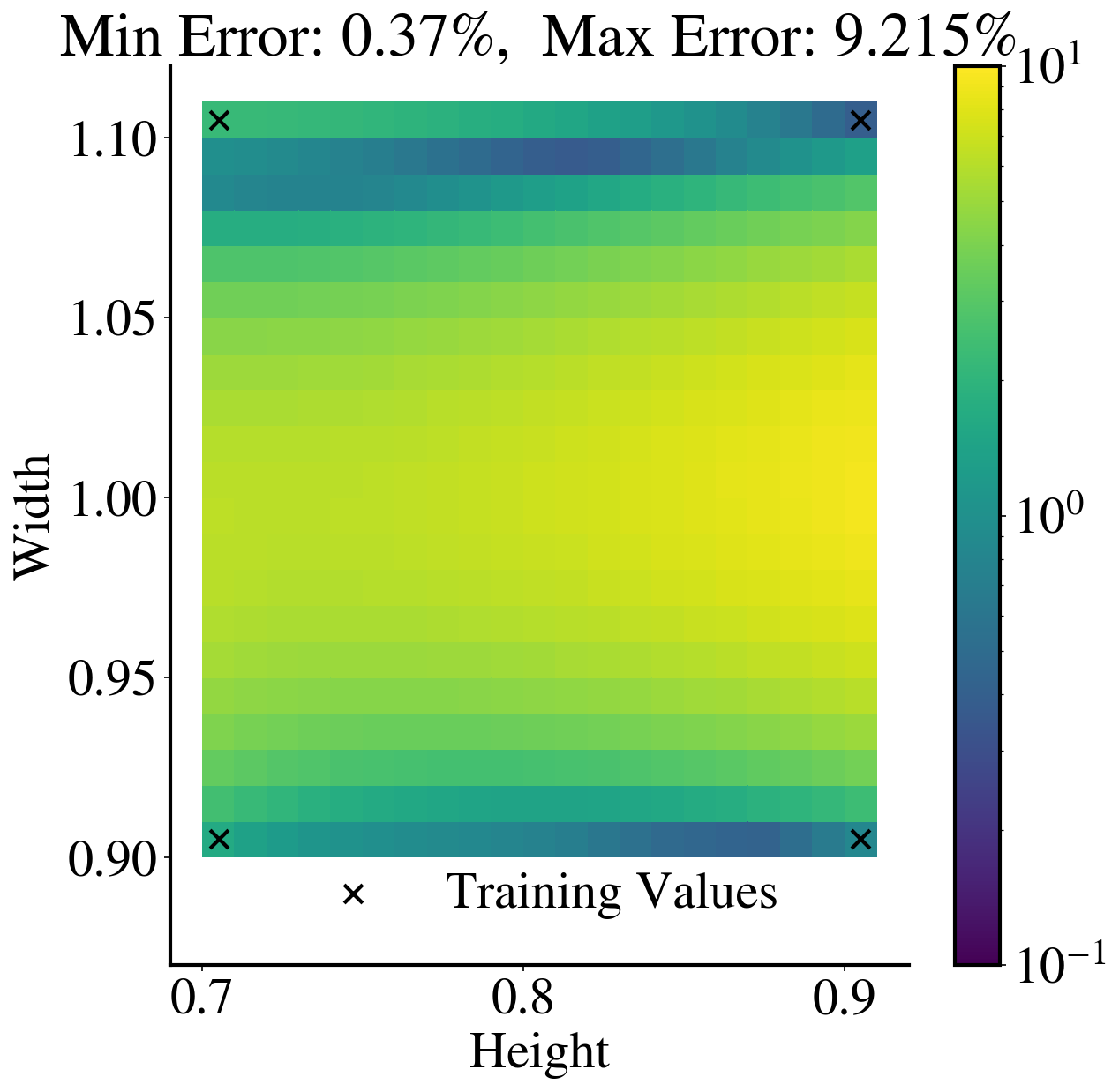
To see the accuracy over the whole parameter domain, Figure 7 shows two heat maps of the maximum relative errors for each parameter case: one for LaSDI-NM and the other for LaSDI-LS. Both LaSDIs are trained using four training points. For this particular experiments, LaSDI-LS outperforms LaSDI-NM in terms of accuracy, i.e., The maximum relative error for LaSDI-NM is , while the maximum relative error for LaSDI-LS is .

For more extensive analysis, we report accuracy (i.e., the relative error range) and speedup for various LaSDI models in Figure 8. We train LaSDI-NM and LaSDI-LS models with nine training points. Then both the region-based and interpolation-based local LaSDIs are constructed for various s, labeled as LaSDI-NM, interpolated LaSDI-NM with RBF, interpolated LaSDI-NM with B-Spline, LaSDI-LS, interpolated LaSDI-LS with RBF, and interpolated LaSDI-LS with B-Spline. Furthermore, we compare both Degree 0 and 1 dynamical system in DIs. There are several things to note. First, the relative ranges for Degree 1 dynamical systems tend to be bigger than the ones for Degree 0 dynamical systems. This makes sense because a lot more variations are possible with a higher degree, which gives a higher chance to be both the best and worst model. As a matter of fact, the best model with the minimum relative error range is found with Degree 1 Dynamical system (i.e., the region-based LaSDI-LS with ). Second, the interpolated LaSDIs tend to give a larger relative error range than the region-based local LaSDIs. We speculate that this is because the training points were not optimally chosen for the interpolation. This fact will be further investigated in the follow-up paper. Third, a higher speed-up is achieved by Degree 0 dynamical system. This also makes sense because the solution process of the latent space dynamics with less degrees will be faster.


In Figure 9, we plot the heat maps of the relative error for the best LaSDI-LS and LaSDI-NM models that are identified from Figure 8, i.e., the LaSDI-NM Global DI and the region-based LaSDI-LS local DI with . The plot reveals that the LaSDI-LS local DI is better than the LaSDI-NM global DI model for this particular case.
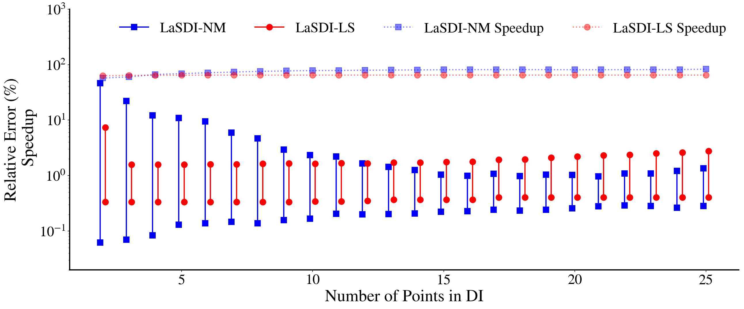
Figure 10 compares the performance of LaSDI-LS and LaSDI-NM with 25 total training points to see the effect of increasing the number of training FOMs. First, the accuracy of LaSDI-NM has been improved when compared with the ones with 4 or 9 training points (see Figures 7 and 9). For example, the maximum relative error of LaSDI-NM has decreased from to and to as the number of training points increase from 4 to 9 and to 25. This implying that more data is used, the better the accuracy of LaSDI-NM would be. Second, while LaSDI-NM gives a larger range of maximum relative errors when 9 training FOMs are used, it consistently gives the smallest relative error of all predictive LaSDIs. Finally, we notice no reduction in error in LaSDI-LS from 9 to 25 training values; this highlights the limitations of POD in advection-dominated problems.
4.2 2D Burgers
We expect that LaSDI-NM will perform better than LaSDI-LS for the 2D Burgers problem based on the singular value decay shown in Figure 3. Figure 11 illustrates the accuracy level achieved by LaSDI models for both the and components of the velocity as well as the relative error at the last time step. The figure shows the clear advantage of LaSDI-NM over LaSDI-LS over the advection-dominated problem, as expected. Of course, the projection error of the linear compression can be improved by increasing the latent space dimension. However, the larger latent space dimension implies the more terms to be identified in the dynamics identification step.

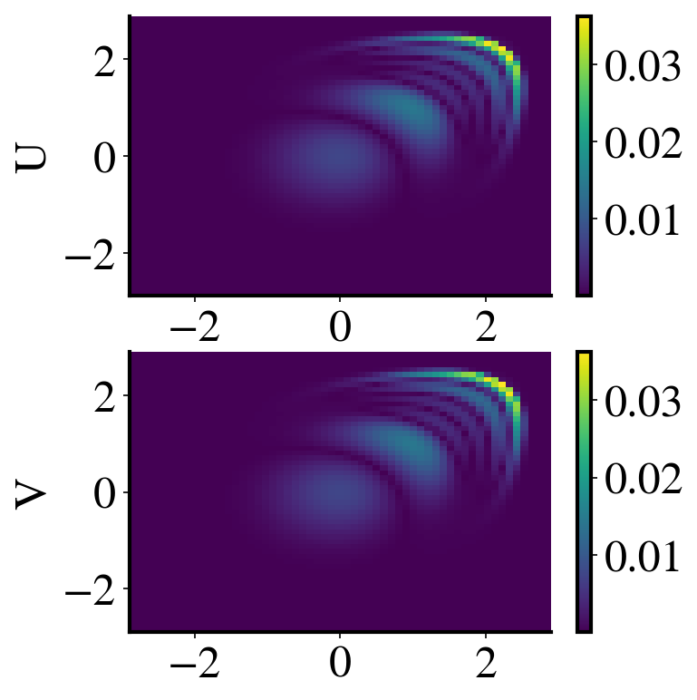
Figure 12 illustrates the relative error of a LaSDI model is bounded below by the projection error of the compression technique.


The comparison between LaSDI-LS and LaSDI-NM becomes even more vivid in Figure 13, which shows the performance of LaSDI models with 25 training points. For this example, we note that the region-based local DI outperforms global DI for LaSDI-NM. This implies that the latent-space dynamics are heavily localized within the parameter space. That is, for example, the dynamical system that best approximates the case of , is not a good model for the case of , .
For this particular problem, a speed-up around 800 is achieved by LaSDI-NM. We use a cubic dynamical system, with cross-terms, to improve the expressivity and therefore accurately represent the three dimensional latent space generated in LaSDI-NM. However, the higher-degree dynamical systems in DI can be numerically unstable. Furthermore, the lower degree approximation can lead to a higher speed-up. Thus, the balance among expressivity, numerical instability, and speed-up must be sought when LaSDI models are applied.
4.3 Time-Dependent Heat Conduction
Based on the singular value decay in Figure 3, we expect that the LaSDI-LS will perform better than the LaSDI-NM. Indeed, Figure 14 shows that the LaSDI-LS achieves much smaller relative error than the LaSDI-NM for and .


As discussed in Section 3.2.1, increasing the dimension of the the latent space necessarily increases the amount of information retained in the data-compression. To quantify this, we track the first singular values as a proportion of the sum of the singular values:
| (27) |
where serves as an indicator for the projection error of the POD-based reduced space as the projection error decreases as increases. As seen in Figures 6 and 12, the projection error of the POD also serves as the lower bound for the LaSDI-LS. Therefore, it would be nice if the accuracy of the LaSDI-LS can follow the trend of the projection error of the POD-based compression. Figure 15 indeed illustrates the relative error range decreases as the latent space dimension increases. This feature implies that the accuracy of LaSDI-LS follows the trend of the projection error for this particular problem.
The decrease in the projection error implies that the quality improvement of the latent space accomplished by the POD. However, the overall accuracy of LaSDI models does not depend only on the quality of the latent space, but also on the quality of the DI model. Therefore, the decay of the relative error range in Figure 15 is possible because the DI models are in good quality as well.
Accurate LaSDI-LS requires fast singular value decay and as we present below, simple latent space dynamics are required to maintain this accuracy (i.e., Figure 16 demonstrates that 0 degree dynamical systems in DI is enough to produce a good accuracy for LaSDI-LS). Although the computational cost for the integration of the ODE and the matrix multiplication to decompress the data increases as we increase , the decrease in LaSDI-LS relative error at the expense of decreased speedup times clearly gives benefits to applications that require a high accuracy.


When expanding across the full parameter space, LaSDI-LS continues to produce lower LaSDI-LS errors than LaSDI-NM, as shown in Figure 16. The LaSDI-NM does not produce accurate results leading to the maximum error of LaSDI-NM, while LaSDI-LS achieves the maximum error. Due to the simplicity of both the linear and nonlinear latent spaces, we do see consistent results between local and global DI. As in Section 4.2, simpler dynamics (i.e., 0-degree dynamical system) was enough to approximate the nonlinear latent space dynamics accurately, also leading to a speed-up of much higher than x.
While further neural network architectures can be explored, we restrict ourselves to the shallow masked network, which gave good performance for the 2D Burgers problem in Section 4.2. Because we expect diffusion-dominated problems to be well-represented in a latent spaces that is constructed by a linear compression, as suggested in Figure 3, exploring various neural network structures for this specific problem becomes counter-productive. Furthermore, nonlinear compression techniques, such as auto-encoders, require more computationally expensive training phase than linear compression techniques, such as POD. We have included the results of LaSDI-NM only to highlight the importance of data compression selection when implementing LaSDI.
4.4 Radial Advection
We show the numerical results for the radial advection problem. As in the previous sections, we first present results of LaSDI models for one specific test point to illustrate the viability of the method. Figure 17 presents the heat maps of relative errors produced by both LaSDI-LS and LaSDI-NM. As expected, LaSDI-NM performs significantly better than LaSDI-LS in terms of accuracy because the problem is advection-dominated and the singular value decay is slow as seen in Figure 3.


We now consider two different parameter spaces; a smaller one () and a larger one () as indicated in Table 2. We seek to analyze how flexible LaSDI can be in larger parameter spaces with potentially nonlinear latent space dynamics. Note that for this example, we only vary one parameter in the initial conditions. Thus, we do not include heat maps but rather graphs of the maximum relative error against the parameter value. We also vary the number of training points in each of these examples. Figure 18 shows the comparison of global and local DI that are trained on and predicted on .
Figure 19 depicts the best-case scenario for each of these cases in terms of accuracy. We note the most accurate regime in each case is local DI. Among the best local LaSDI models, as expected, the smaller parameter space with the larger number of training points performs the best, with a maximum relative error of . Likewise, the worst result appears in the larger parameter space with the smaller number of training points. In this case LaSDI-NM reaches error approximately 20%.
Interestingly, the local LaSDI (2) DI model on (i.e., Figure 19(b)) outperforms the local LaSDI (3) DI model on (i.e, Figure 19(c)) when using LaSDI-NM. This implies that local LaSDI models will perform well as long as there are enough training points whether the parameter space is large or small. On the other hand, the performance of the global LaSDI-NM models is affected by the parameter space size. For example, the worst error of the global LaSDI-NM for is , while the worst error of the global LaSDI-NM for is .


5 Conclusion
We have introduced a framework for latent space dynamics identification (LaSDI) that builds efficient parametric models by exploiting both local and global regression techniques. Two types of local dynamics identification models are introduced: (i) region-based and (ii) point-wise interpolated DIs. Latent spaces are generated in two different ways as well, i.e., using linear and nonlinear compression techniques. The compression techniques, such as proper orthogonal decomposition and auto-encoder, reduce large-scale simulation data to small-scale data whose size is manageable for regression techniques. The framework is general enough to be applicable to any physical simulations. We have applied various LaSDI models to four different problems, i.e., 1D and 2D Burgers, heat conduction, and radial advection problems.
We observe that local versus global DI models need to be determined case by case. For example, a local DI model outperforms global DI for LaSDI-NM for 1D Burgers problem with nine training points (see the case of Degree 0 dynamical system in Figure 8) and 2D Burgers problem with 25 training points (see Figure 13) and all the cases for radial advection problems (see Figure 18), while a global DI or local DI with larger number of points outperform a local DI with smaller number of points for LaSDI-NM for 1D Burgers problem with 25 training points (see Figure 10).
The nonlinear compression techniques, such as auto-encoder, outperforms the linear compression technique for problems with slowly decaying Kolmogorov’s width, while the linear compression techniques, such as proper orthogonal decomposition, outperforms the nonlinear compression technique for problems with fast decaying Kolmogorov’s width. The nonlinear compression was able to bring the projection error down with small latent space dimension even for the problems with slowly decaying Komogorov’s width. However, the computational cost of the nonlinear manifold compression is much higher than the linear compression, so we recommend using linear compression if the problem shows fast singular value decay.
There are several future directions to consider in the context of latent space dynamics identification framework. First, we have only considered predefined uniformly distributed training parameters, which is fine with a small size parameter space dimension of one or two. However, the number of uniformly distributed training points increases exponentially as the dimension of the parameter space increases, which makes the generation of the simulation data extremely challenging. Therefore, adaptive and sparse parameter sampling for LaSDI needs to be developed, which will lead to an optimal sampling. Second, we have only considered the parameters that affects an initial condition. However, a parameter of interest may not alter the initial condition, e.g., material properties. The LaSDI framework introduced in this paper cannot handle this case. Therefore, parameterization other than the initial condition needs to be developed. Third, we have extensively used a regression technique to identify dynamics in a latent space. However, this is not the only option. For example, any system identification techniques or operator learning algorithms are applicable. Fourth, the architecture of the neural network for LaSDI-NM may not have been optimally chosen. The more thorough neural architecture search would lead to the better performance of LaSDI-NM models. Finally, because LaSDI is a non-intrusive method, it can be applied to data sets that might not be generated by simulations. These methods, along with adding regularization to the training process can help discover more robust latent-space dynamical systems for potentially noisy and imperfect data as done in [50].
With these future directions, the potential for LaSDI is to offer fast and accurate data-driven simulation capability. We expect to apply LaSDI to various important applications, such as climate science, manufacturing, and fusion energy.
Acknowledgments
This work was performed at Lawrence Livermore National Laboratory and partially funded by two LDRDs (21-FS-042 and 21-SI-006). Lawrence Livermore National Laboratory is operated by Lawrence Livermore National Security, LLC, for the U.S. Department of Energy, National Nuclear Security Administration under Contract DE-AC52-07NA27344 and LLNL-JRNL-831849.
This research was supported in part by an appointment with the National Science Foundation (NSF) Mathematical Sciences Graduate Internship (MSGI) Program sponsored by the NSF Division of Mathematical Sciences. This program is administered by the Oak Ridge Institute for Science and Education (ORISE) through an interagency agreement between the U.S. Department of Energy (DOE) and NSF. ORISE is managed for DOE by ORAU. All opinions expressed in this paper are the author’s and do not necessarily reflect the policies and views of NSF, ORAU/ORISE, or DOE.
References
- [1] G. Berkooz, P. Holmes, and J. L. Lumley, “The proper orthogonal decomposition in the analysis of turbulent flows,” Annual review of fluid mechanics, vol. 25, no. 1, pp. 539–575, 1993.
- [2] A. T. Patera, G. Rozza, et al., “Reduced basis approximation and a posteriori error estimation for parametrized partial differential equations,” 2007.
- [3] M. G. Safonov and R. Chiang, “A schur method for balanced-truncation model reduction,” IEEE Transactions on automatic control, vol. 34, no. 7, pp. 729–733, 1989.
- [4] Y. Kim, Y. Choi, D. Widemann, and T. Zohdi, “A fast and accurate physics-informed neural network reduced order model with shallow masked autoencoder,” Journal of Computational Physics, p. 110841, 2021.
- [5] Y. Kim, Y. Choi, D. Widemann, and T. Zohdi, “Efficient nonlinear manifold reduced order model,” arXiv preprint arXiv:2011.07727, 2020.
- [6] R. Maulik, B. Lusch, and P. Balaprakash, “Reduced-order modeling of advection-dominated systems with recurrent neural networks and convolutional autoencoders,” Physics of Fluids, vol. 33, no. 3, p. 037106, 2021.
- [7] K. Lee and K. T. Carlberg, “Model reduction of dynamical systems on nonlinear manifolds using deep convolutional autoencoders,” Journal of Computational Physics, vol. 404, p. 108973, 2020.
- [8] D. M. Copeland, S. W. Cheung, K. Huynh, and Y. Choi, “Reduced order models for lagrangian hydrodynamics,” Computer Methods in Applied Mechanics and Engineering, vol. 388, p. 114259, 2022.
- [9] S. W. Cheung, Y. Choi, D. M. Copeland, and K. Huynh, “Local lagrangian reduced-order modeling for rayleigh-taylor instability by solution manifold decomposition,” arXiv preprint arXiv:2201.07335, 2022.
- [10] Y. Choi, D. Coombs, and R. Anderson, “Sns: a solution-based nonlinear subspace method for time-dependent model order reduction,” SIAM Journal on Scientific Computing, vol. 42, no. 2, pp. A1116–A1146, 2020.
- [11] Y. Choi and K. Carlberg, “Space–time least-squares petrov–galerkin projection for nonlinear model reduction,” SIAM Journal on Scientific Computing, vol. 41, no. 1, pp. A26–A58, 2019.
- [12] K. Carlberg, Y. Choi, and S. Sargsyan, “Conservative model reduction for finite-volume models,” Journal of Computational Physics, vol. 371, pp. 280–314, 2018.
- [13] C. Hoang, Y. Choi, and K. Carlberg, “Domain-decomposition least-squares petrov–galerkin (dd-lspg) nonlinear model reduction,” Computer Methods in Applied Mechanics and Engineering, vol. 384, p. 113997, 2021.
- [14] Y. Choi, G. Boncoraglio, S. Anderson, D. Amsallem, and C. Farhat, “Gradient-based constrained optimization using a database of linear reduced-order models,” Journal of Computational Physics, vol. 423, p. 109787, 2020.
- [15] T. Iliescu and Z. Wang, “Variational multiscale proper orthogonal decomposition: Navier-stokes equations,” Numerical Methods for Partial Differential Equations, vol. 30, no. 2, pp. 641–663, 2014.
- [16] D. Amsallem and C. Farhat, “Interpolation method for adapting reduced-order models and application to aeroelasticity,” AIAA journal, vol. 46, no. 7, pp. 1803–1813, 2008.
- [17] Y. Kim, K. Wang, and Y. Choi, “Efficient space–time reduced order model for linear dynamical systems in python using less than 120 lines of code,” Mathematics, vol. 9, no. 14, p. 1690, 2021.
- [18] Y. Choi, P. Brown, W. Arrighi, R. Anderson, and K. Huynh, “Space–time reduced order model for large-scale linear dynamical systems with application to boltzmann transport problems,” Journal of Computational Physics, vol. 424, p. 109845, 2021.
- [19] Y. Choi, G. Oxberry, D. White, and T. Kirchdoerfer, “Accelerating design optimization using reduced order models,” arXiv preprint arXiv:1909.11320, 2019.
- [20] D. Amsallem, M. Zahr, Y. Choi, and C. Farhat, “Design optimization using hyper-reduced-order models,” Structural and Multidisciplinary Optimization, vol. 51, no. 4, pp. 919–940, 2015.
- [21] S. McBane and Y. Choi, “Component-wise reduced order model lattice-type structure design,” Computer Methods in Applied Mechanics and Engineering, vol. 381, p. 113813, 2021.
- [22] G. Tapia, S. Khairallah, M. Matthews, W. E. King, and A. Elwany, “Gaussian process-based surrogate modeling framework for process planning in laser powder-bed fusion additive manufacturing of 316l stainless steel,” The International Journal of Advanced Manufacturing Technology, vol. 94, no. 9, pp. 3591–3603, 2018.
- [23] Z. Qian, C. C. Seepersad, V. R. Joseph, J. K. Allen, and C. F. Jeff Wu, “Building Surrogate Models Based on Detailed and Approximate Simulations,” Journal of Mechanical Design, vol. 128, pp. 668–677, 06 2005.
- [24] B. Daniel Marjavaara, T. Staffan Lundström, T. Goel, Y. Mack, and W. Shyy, “Hydraulic Turbine Diffuser Shape Optimization by Multiple Surrogate Model Approximations of Pareto Fronts,” Journal of Fluids Engineering, vol. 129, pp. 1228–1240, 04 2007.
- [25] F. Huang, L. Wang, and C. Yang, “Hull form optimization for reduced drag and improved seakeeping using a surrogate-based method,” in The Twenty-fifth International Ocean and Polar Engineering Conference, OnePetro, 2015.
- [26] Z.-H. Han, S. Görtz, and R. Zimmermann, “Improving variable-fidelity surrogate modeling via gradient-enhanced kriging and a generalized hybrid bridge function,” Aerospace Science and technology, vol. 25, no. 1, pp. 177–189, 2013.
- [27] Z.-H. Han and S. Görtz, “Hierarchical kriging model for variable-fidelity surrogate modeling,” AIAA journal, vol. 50, no. 9, pp. 1885–1896, 2012.
- [28] X. Guo, W. Li, and F. Iorio, “Convolutional neural networks for steady flow approximation,” in Proceedings of the 22nd ACM SIGKDD international conference on knowledge discovery and data mining, pp. 481–490, 2016.
- [29] Y. Zhang, W. J. Sung, and D. N. Mavris, “Application of convolutional neural network to predict airfoil lift coefficient,” in 2018 AIAA/ASCE/AHS/ASC Structures, Structural Dynamics, and Materials Conference, p. 1903, 2018.
- [30] M. Paganini, L. de Oliveira, and B. Nachman, “Calogan: Simulating 3d high energy particle showers in multilayer electromagnetic calorimeters with generative adversarial networks,” Physical Review D, vol. 97, no. 1, p. 014021, 2018.
- [31] J. Peurifoy, Y. Shen, L. Jing, Y. Yang, F. Cano-Renteria, B. G. DeLacy, J. D. Joannopoulos, M. Tegmark, and M. Soljačić, “Nanophotonic particle simulation and inverse design using artificial neural networks,” Science advances, vol. 4, no. 6, p. eaar4206, 2018.
- [32] T. Kadeethum, D. O’Malley, J. N. Fuhg, Y. Choi, J. Lee, H. S. Viswanathan, and N. Bouklas, “A framework for data-driven solution and parameter estimation of pdes using conditional generative adversarial networks,” arXiv preprint arXiv:2105.13136, 2021.
- [33] T. Kadeethum, D. O’Malley, Y. Choi, H. S. Viswanathan, N. Bouklas, and H. Yoon, “Continuous conditional generative adversarial networks for data-driven solutions of poroelasticity with heterogeneous material properties,” arXiv preprint arXiv:2111.14984, 2021.
- [34] T. Kadeethum, F. Ballarin, Y. Choi, D. O’Malley, H. Yoon, and N. Bouklas, “Non-intrusive reduced order modeling of natural convection in porous media using convolutional autoencoders: comparison with linear subspace techniques,” arXiv preprint arXiv:2107.11460, 2021.
- [35] Y. Zhu and N. Zabaras, “Bayesian deep convolutional encoder–decoder networks for surrogate modeling and uncertainty quantification,” Journal of Computational Physics, vol. 366, pp. 415–447, 2018.
- [36] S.-W. Kim, J. A. Melby, N. C. Nadal-Caraballo, and J. Ratcliff, “A time-dependent surrogate model for storm surge prediction based on an artificial neural network using high-fidelity synthetic hurricane modeling,” Natural Hazards, vol. 76, no. 1, pp. 565–585, 2015.
- [37] J. N. Kutz, “Deep learning in fluid dynamics,” Journal of Fluid Mechanics, vol. 814, pp. 1–4, 2017.
- [38] J. Marçais and J.-R. de Dreuzy, “Prospective interest of deep learning for hydrological inference,” Groundwater, vol. 55, no. 5, pp. 688–692, 2017.
- [39] S. Chan and A. H. Elsheikh, “A machine learning approach for efficient uncertainty quantification using multiscale methods,” Journal of Computational Physics, vol. 354, pp. 493–511, 2018.
- [40] S. Min, B. Lee, and S. Yoon, “Deep learning in bioinformatics,” Briefings in bioinformatics, vol. 18, no. 5, pp. 851–869, 2017.
- [41] P. Baldi, P. Sadowski, and D. Whiteson, “Searching for exotic particles in high-energy physics with deep learning,” Nature communications, vol. 5, no. 1, pp. 1–9, 2014.
- [42] J.-X. Wang, J. Wu, J. Ling, G. Iaccarino, and H. Xiao, “A comprehensive physics-informed machine learning framework for predictive turbulence modeling,” arXiv preprint arXiv:1701.07102, 2017.
- [43] E. J. Parish and K. Duraisamy, “A paradigm for data-driven predictive modeling using field inversion and machine learning,” Journal of Computational Physics, vol. 305, pp. 758–774, 2016.
- [44] K. Duraisamy, Z. J. Zhang, and A. P. Singh, “New approaches in turbulence and transition modeling using data-driven techniques,” in 53rd AIAA Aerospace Sciences Meeting, p. 1284, 2015.
- [45] J. Ling, A. Kurzawski, and J. Templeton, “Reynolds averaged turbulence modelling using deep neural networks with embedded invariance,” Journal of Fluid Mechanics, vol. 807, pp. 155–166, 2016.
- [46] R. K. Tripathy and I. Bilionis, “Deep uq: Learning deep neural network surrogate models for high dimensional uncertainty quantification,” Journal of computational physics, vol. 375, pp. 565–588, 2018.
- [47] T. Hagge, P. Stinis, E. Yeung, and A. M. Tartakovsky, “Solving differential equations with unknown constitutive relations as recurrent neural networks,” arXiv preprint arXiv:1710.02242, 2017.
- [48] P. R. Vlachas, W. Byeon, Z. Y. Wan, T. P. Sapsis, and P. Koumoutsakos, “Data-driven forecasting of high-dimensional chaotic systems with long short-term memory networks,” Proceedings of the Royal Society A: Mathematical, Physical and Engineering Sciences, vol. 474, no. 2213, p. 20170844, 2018.
- [49] J. Morton, F. D. Witherden, A. Jameson, and M. J. Kochenderfer, “Deep dynamical modeling and control of unsteady fluid flows,” arXiv preprint arXiv:1805.07472, 2018.
- [50] B. Chen, K. Huang, S. Raghupathi, I. Chandratreya, Q. Du, and H. Lipson, “Discovering state variables hidden in experimental data,” 2021.
- [51] B. Kim, V. C. Azevedo, N. Thuerey, T. Kim, M. Gross, and B. Solenthaler, “Deep fluids: A generative network for parameterized fluid simulations,” Computer Graphics Forum, vol. 38, p. 59–70, May 2019.
- [52] S. Fresca, L. Dede, and A. Manzoni, “A comprehensive deep learning-based approach to reduced order modeling of nonlinear time-dependent parametrized pdes,” Journal of Scientific Computing, vol. 87, no. 2, pp. 1–36, 2021.
- [53] X. Xie, G. Zhang, and C. G. Webster, “Non-intrusive inference reduced order model for fluids using deep multistep neural network,” Mathematics, vol. 7, no. 8, p. 757, 2019.
- [54] C. Hoang, K. Chowdhary, K. Lee, and J. Ray, “Projection-based model reduction of dynamical systems using space–time subspace and machine learning,” Computer Methods in Applied Mechanics and Engineering, p. 114341, 2021.
- [55] K. Champion, B. Lusch, J. N. Kutz, and S. L. Brunton, “Data-driven discovery of coordinates and governing equations,” Proceedings of the National Academy of Sciences, vol. 116, no. 45, pp. 22445–22451, 2019.
- [56] P. J. Schmid, “Dynamic mode decomposition of numerical and experimental data,” Journal of fluid mechanics, vol. 656, pp. 5–28, 2010.
- [57] J. H. Tu, Dynamic mode decomposition: Theory and applications. PhD thesis, Princeton University, 2013.
- [58] J. L. Proctor, S. L. Brunton, and J. N. Kutz, “Dynamic mode decomposition with control,” SIAM Journal on Applied Dynamical Systems, vol. 15, no. 1, pp. 142–161, 2016.
- [59] P. J. Schmid, L. Li, M. P. Juniper, and O. Pust, “Applications of the dynamic mode decomposition,” Theoretical and Computational Fluid Dynamics, vol. 25, no. 1, pp. 249–259, 2011.
- [60] J. N. Kutz, S. L. Brunton, B. W. Brunton, and J. L. Proctor, Dynamic mode decomposition: data-driven modeling of complex systems. SIAM, 2016.
- [61] P. J. Schmid, “Dynamic mode decomposition and its variants,” Annual Review of Fluid Mechanics, vol. 54, pp. 225–254, 2022.
- [62] J. N. Kutz, X. Fu, and S. L. Brunton, “Multiresolution dynamic mode decomposition,” SIAM Journal on Applied Dynamical Systems, vol. 15, no. 2, pp. 713–735, 2016.
- [63] P. J. Schmid, “Application of the dynamic mode decomposition to experimental data,” Experiments in fluids, vol. 50, no. 4, pp. 1123–1130, 2011.
- [64] S. Le Clainche and J. M. Vega, “Higher order dynamic mode decomposition,” SIAM Journal on Applied Dynamical Systems, vol. 16, no. 2, pp. 882–925, 2017.
- [65] D. Duke, J. Soria, and D. Honnery, “An error analysis of the dynamic mode decomposition,” Experiments in fluids, vol. 52, no. 2, pp. 529–542, 2012.
- [66] M. R. Jovanović, P. J. Schmid, and J. W. Nichols, “Sparsity-promoting dynamic mode decomposition,” Physics of Fluids, vol. 26, no. 2, p. 024103, 2014.
- [67] N. Demo, M. Tezzele, and G. Rozza, “Pydmd: Python dynamic mode decomposition,” Journal of Open Source Software, vol. 3, no. 22, p. 530, 2018.
- [68] M. S. Hemati, M. O. Williams, and C. W. Rowley, “Dynamic mode decomposition for large and streaming datasets,” Physics of Fluids, vol. 26, no. 11, p. 111701, 2014.
- [69] N. B. Erichson, L. Mathelin, J. N. Kutz, and S. L. Brunton, “Randomized dynamic mode decomposition,” SIAM Journal on Applied Dynamical Systems, vol. 18, no. 4, pp. 1867–1891, 2019.
- [70] B. Peherstorfer and K. Willcox, “Data-driven operator inference for nonintrusive projection-based model reduction,” Computer Methods in Applied Mechanics and Engineering, vol. 306, pp. 196–215, 2016.
- [71] R. Geelen, S. Wright, and K. Willcox, “Operator inference for non-intrusive model reduction with nonlinear manifolds,” arXiv preprint arXiv:2205.02304, 2022.
- [72] M. Guo, S. McQuarrie, and K. Willcox, “Bayesian operator inference for data-driven reduced order modeling,” arXiv preprint arXiv:2204.10829, 2022.
- [73] R. Geelen and K. Willcox, “Localized non-intrusive reduced-order modeling in the operator inference framework,”
- [74] S. A. McQuarrie, P. Khodabakhshi, and K. E. Willcox, “Non-intrusive reduced-order models for parametric partial differential equations via data-driven operator inference,” arXiv preprint arXiv:2110.07653, 2021.
- [75] E. Qian, B. Kramer, B. Peherstorfer, and K. Willcox, “Lift & learn: Physics-informed machine learning for large-scale nonlinear dynamical systems,” Physica D: Nonlinear Phenomena, vol. 406, p. 132401, 2020.
- [76] R. Swischuk, B. Kramer, C. Huang, and K. Willcox, “Learning physics-based reduced-order models for a single-injector combustion process,” AIAA Journal, vol. 58, no. 6, pp. 2658–2672, 2020.
- [77] P. Benner, P. Goyal, B. Kramer, B. Peherstorfer, and K. Willcox, “Operator inference for non-intrusive model reduction of systems with non-polynomial nonlinear terms,” Computer Methods in Applied Mechanics and Engineering, vol. 372, p. 113433, 2020.
- [78] P. Jain, S. McQuarrie, and B. Kramer, “Performance comparison of data-driven reduced models for a single-injector combustion process,” in AIAA Propulsion and Energy 2021 Forum, p. 3633, 2021.
- [79] S. A. McQuarrie, C. Huang, and K. E. Willcox, “Data-driven reduced-order models via regularised operator inference for a single-injector combustion process,” Journal of the Royal Society of New Zealand, vol. 51, no. 2, pp. 194–211, 2021.
- [80] B. Peherstorfer, “Sampling low-dimensional markovian dynamics for preasymptotically recovering reduced models from data with operator inference,” SIAM Journal on Scientific Computing, vol. 42, no. 5, pp. A3489–A3515, 2020.
- [81] P. Khodabakhshi and K. E. Willcox, “Non-intrusive data-driven model reduction for differential–algebraic equations derived from lifting transformations,” Computer Methods in Applied Mechanics and Engineering, vol. 389, p. 114296, 2022.
- [82] S. Yıldız, P. Goyal, P. Benner, and B. Karasözen, “Learning reduced-order dynamics for parametrized shallow water equations from data,” International Journal for Numerical Methods in Fluids, vol. 93, no. 8, pp. 2803–2821, 2021.
- [83] L. Sirovich, “Turbulence and the dynamics of coherent structures, parts i, ii and iii,” Quart. Appl. Math., pp. 561–590, 1987.
- [84] S. L. Brunton, J. L. Proctor, and J. N. Kutz, “Discovering governing equations from data by sparse identification of nonlinear dynamical systems,” Proceedings of the National Academy of Sciences, vol. 113, no. 15, pp. 3932–3937, 2016.
- [85] J. R. Dormand and P. J. Prince, “A family of embedded runge-kutta formulae,” Journal of computational and applied mathematics, vol. 6, no. 1, pp. 19–26, 1980.
- [86] X. He, Y. Choi, W. D. Fries, J. Belof, and J.-S. Chen, “gLaSDI: Parametric Physics-informed Greedy Latent Space Dynamics Identification,” arXiv preprint arXiv:2204.12005, 2022.
- [87] C. A. Kennedy and M. H. Carpenter, Diagonally Implicit Runge-Kutta methods for ordinary differential equations, a review. National Aeronautics and Space Administration, Langley Research Center, 2016.