Largest eigenvalue of the configuration model
and breaking of ensemble equivalence

Spectral properties of adjacency matrices in random graphs play a crucial role in various areas of network science. The largest eigenvalue is particularly sensitive to the graph architecture, making it a key focus. In this paper we focus on a random graph with a hard constraint on the degrees of nodes. In the homogeneous case (all degrees equal to $d$), it reduces to a random $d$-regular graph. In the heterogeneous case (different degrees), it is known as the configuration model. Our interest is characterizing the expected largest eigenvalue of the configuration model and comparing it with the same quantity for a corresponding random graph model where the degrees are treated as soft constraints.

The set of $d$-regular graphs on $n$ vertices, with $d=d(n)$, is non-empty when $1\leq d\leq n-1$ and $dn$ is even. Selecting a graph uniformly at random from this set results in what is known as the random $d$-regular graph, denoted by $G_{n,d}$. The spectral properties of $G_{n,d}$ are well-studied for $d\geq 2$ (for $d=1$, the graph is trivially a set of disconnected edges). For instance, all eigenvalues of its adjacency matrix fall in the interval $[-d,d]$, with the largest eigenvalue being $d$. The computation of $\lambda=\max\{|\lambda_{2}|,|\lambda_{n}|\}$, where $\lambda_{2}$ and $\lambda_{n}$ are the second-largest and the smallest eigenvalue, respectively, has been challenging. It is well known that for fixed $d$ the empirical distribution function of the eigenvalues of $G_{n,d}$ converges to the so-called Kesten-McKay law [22], the density of which is given by

A lower bound of the type $\lambda\geq 2\sqrt{d-1}$ was expected from this, and was indeed proven in the celebrated Alon-Boppana theorem in [1], stating that $\lambda\geq 2\sqrt{d-1}+O_{d}(\log^{-2}(n))$, where the constant in the error term only depends on $d$. In the same paper an upper bound of the type $\lambda\leq 2\sqrt{d-1}+o(1)$ was conjectured . This conjecture was later proven in the pioneering work [17] (for a shorter proof, see [6]). When $d=d(n)\to\infty$, the spectral distribution converges to the semi-circular law [26]. It was proven in [10] that $\lambda=O(\sqrt{d}\,)$ with high probability when $d=o(\sqrt{n}\,)$. This result was extended in [3] to $d=o(n^{2/3})$. For recent results and open problems, we refer the reader to [30].

There has not been much work on the inhomogeneous setting where not all the degrees of the graph are the same. The natural extension of the regular random graph is the configuration model, where a degree sequence $\vec{d}_{n}=(d_{1},\ldots,d_{n})$ is prescribed. Unless otherwise specified, we assume the degrees to be hard constraints, i.e. realized exactly on each configuration of the model (this is sometimes called the ‘microcanonical’ configuration model, as opposed to the ‘canonical’ one where the degrees are soft constraints realized only as ensemble averages [24, 20]). The empirical spectral distribution of the configuration model is known under some assumptions on the growth of the sum of the degrees. When $\sum_{i=1}^{n}d_{i}=O(n)$, the graph locally looks like a tree. It has been shown that the empirical spectral distribution exists and that the limiting measure is a functional of a size-biased Galton-Watson tree [7]. When $\sum_{i=1}^{n}d_{i}$ grows polynomially with $n$, the local geometry is no longer a tree. This case was recently studied in [12], where it is shown that the appropriately scaled empirical spectral distribution of the configuration model converges to the free multiplicative convolution of the semi-circle law with a measure that depends on the empirical degree sequence. The scaling of the largest and the second-largest eigenvalues has not yet been studied in full generality.

For the configuration model the behaviour of the largest eigenvalue is non-trivial. In the present paper, we consider the configuration model with large degrees, compute the expectation of the largest eigenvalue of its adjacency matrix, and prove a weak law of large numbers. When $d\to\infty$, the empirical distribution of $G_{n,d}$ (appropriately scaled) converges to the semi-circle law. Also, if we look at Erdős-Rényi random graphs on $n$ vertices with connection probability $d/n$, then the appropriately scaled empirical distribution converges to the semi-circle law. It is known that the latter two random graphs exhibit different behaviour for the expected largest eigenvalue [13]. This can be understood in the broader perspective of breaking ensemble equivalence [24, 20], which we discuss later. In the inhomogeneous setting, the natural graph to compare the configuration model with is the Chung-Lu model. For the case where the sum of the degrees grows with $n$, it was shown in [11] that the empirical spectral distribution converges to the free multiplicative product of the semi-circle law with a measure that depends on the degree sequence, similar to [12]. In [14], we investigated the largest eigenvalue and its expectation for the Chung-Lu model (and even derived a central limit theorem). In the present paper we complete the picture by showing that, when the degrees are large, there is a gap between the expected largest eigenvalue of the Chung-Lu model and the configuration model. We refer the reader to the references listed in [13, 14] for more background.

For $n\in\mathbb{N}$, let $\mathrm{CM}(\vec{d}_{n})$ be the random graph on $n$ vertices generated according to the configuration model with degree sequence $\vec{d}_{n}=(d_{i})_{i\in[n]}\in\mathbb{N}^{n}$ [27, Chapter 7.2]. Define

Throughout the paper we need the following assumptions on $\vec{d}_{n}$ as $n\to\infty$.

Let $A_{\mathrm{CM}(\vec{d}_{n})}$ be the adjacency matrix of $\mathrm{CM}(\vec{d}_{n})$. Let $(\lambda_{i})_{i\in[n]}$ be the eigenvalues of $A_{\mathrm{CM}(\vec{d}_{n})}$, ordered such that $\lambda_{1}\geq\dots\geq\lambda_{n}$. We are interested in the behaviour of $\lambda_{1}$ as $n\to\infty$. Our main theorem reads as follows.

In [14] we looked at an alternative version of the configuration model, called the Chung-Lu model $\mathrm{CM}^{*}_{n}(\vec{d}_{n})$, where the average degrees, rather than the degrees themselves, are fixed at $\vec{d}_{n}$. This is an ensemble with soft constraints; in the considered regime for the degrees, it coincides with a maximum-entropy ensemble, also called ‘canonical’ configuration model [24]. For this model we showed that, subject to Assumption 1.1,

and $\lambda_{1}/\mathbb{E}^{*}\left[\lambda_{1}\right]\to 1$ in $\mathbb{P}^{*}$-probability, where $\mathbb{P}^{*}$ and $\mathbb{E}^{*}$ denote expectation with respect to the law of $\mathrm{CM}^{*}_{n}(\vec{d}_{n})$ and $\lambda_{1}$ is the largest eigenvalue of the $A_{\mathrm{CM}^{*}_{n}(\vec{d}_{n})}$. The notable difference between (1.1) and (1.2) is the shift by $-1$.

For the special case where all the degrees are equal to $d$, we have $m_{0}=m_{\infty}=d$ and $m_{k}=nd^{k}$, and so $\mathbb{E}[\lambda_{1}]=d+o(1)$ and $\mathbb{E}^{*}[\lambda_{1}]=d+1+o(1)$. In fact, $\mathbb{P}(\lambda_{1}=d)=1$. Since in this model the degrees can fluctuate with the same law (soft constraint in the physics literature), this case reduces to the Erdős-Rényi random graph for which results on $\mathbb{E}^{*}[\lambda_{1}]$ were already well known in [21, 19] and further analyzed in [15].

The shift by $-1$ was proven in [13] for the homogeneous case with equal degrees and is a spectral signature of breaking of ensemble equivalence [24]. Indeed, a $d$-regular graph is the ‘micro-canonical’ version of a random graph where all degrees are equal and ‘hard’, and the Erdős-Rényi random graph is the corresponding ‘canonical’ version where all degrees are equal and ‘soft’. More in general, $\mathrm{CM}(\vec{d}_{n})$ is the micro-canonical configuration model where the constraint on the degrees is ‘hard’, while $\mathrm{CM}^{*}_{n}(\vec{d}_{n})$ is the canonical version where the constraint is ‘soft’. We refer the reader to [20] for the precise definition of these two configuration model ensembles and for the proof that they are not asymptotically equivalent in the measure sense [25]. This means that the relative entropy per node of $\mathbb{P}$ with respect to $\mathbb{P}^{*}$ has a strictly positive limit as $n\to\infty$. This shows that the choice of constraint matters, not only on a microscopic scale but also on a macroscopic scale. Indeed, for non-equivalent ensembles one expects the existence of certain macroscopic properties that have different expectation values in the two ensembles (macrostate (in)equivalence [25]). The fact that the largest eigenvalue picks up this discrepancy is interesting. What is remarkable is that the shift by $-1$, under the hypotheses considered, holds true also in the case of heterogeneous degrees and remains the same irrespective of the scale of the degrees and of the distribution of the degrees on this scale.

The remainder of this paper is organised as follows. In Section 2 we look at the issue of simplicity of the graph. In Section 3 we bound the spectral norm of the matrix

We use the proof of [10] to show that $\|H\|=\mathrm{o}(m_{\infty})$ with high probability. Using the latter we show that

with high probability. In Section 4 we use the estimates in Section 3 to prove Theorem 1.2.

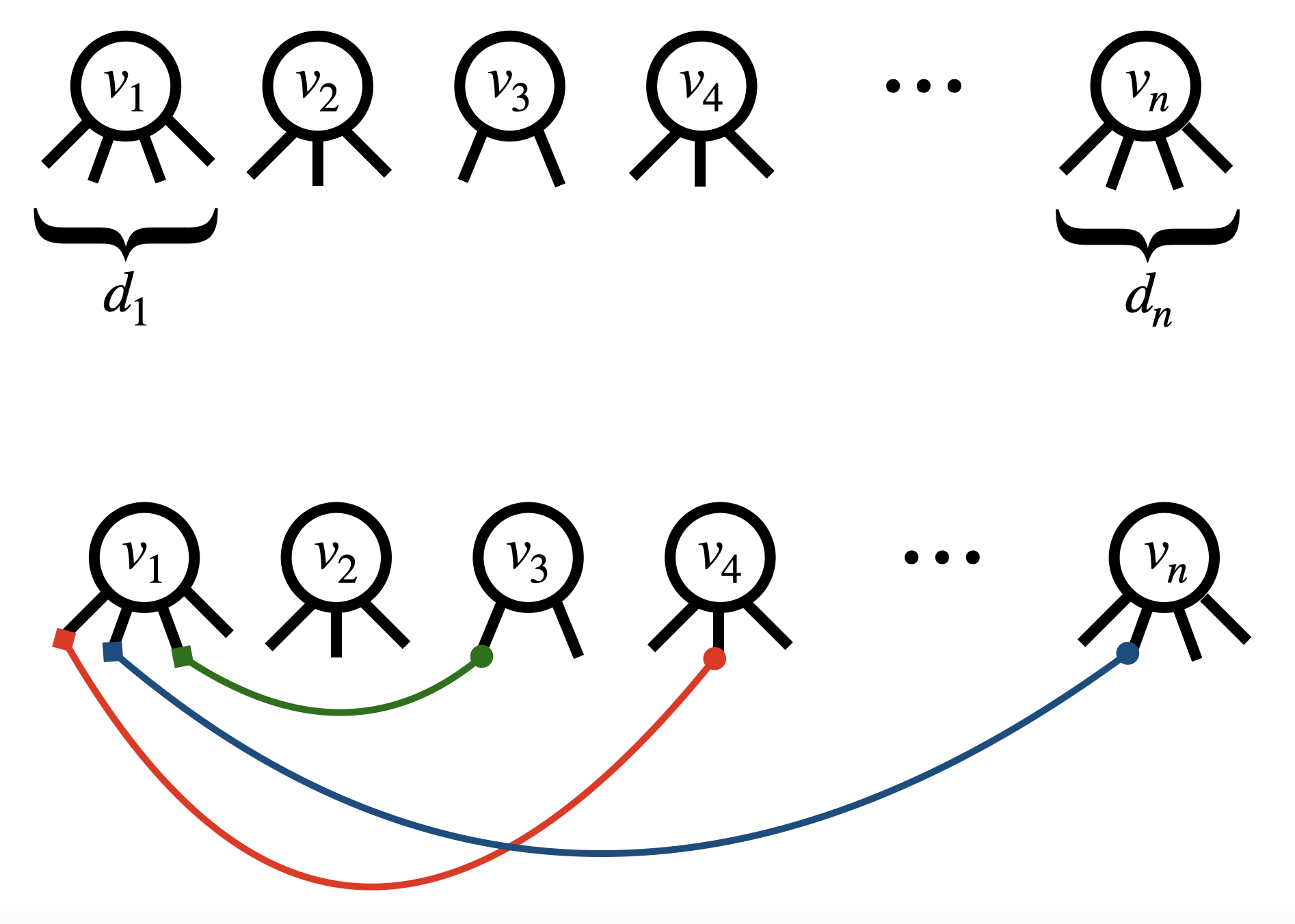
The configuration model with degree sequence $\vec{d}=(d_{1},\dots,d_{n})$, $\mathrm{CM}(\vec{d}_{n})$, generates a graph through a perfect matching $P$ of the set of half-edges $\mathcal{E}=\cup_{i\in[n]}\{i\}\times[d_{i}]$, i.e., $P\colon\,\mathcal{E}\to\mathcal{E}$ such that $P$ is an isomorphism and an involution, and $P(\alpha)\neq\alpha$ for all $\alpha\in\mathcal{E}$.

It turns out that a pairing scheme, such as matching half-edges from left to right or selecting pairs uniformly at random, is considered admissible as long as it yields the correct probability for a perfect matching (see, for example, [27, Lemma 7.6]). An important property of each admissible pairing scheme is that

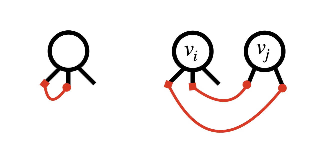
We can therefore endow $\mathcal{E}$ with the lexicographic order. An element $\alpha\in\mathcal{E}$, $\alpha=(i,\ell)$, is associated with a vertex $v(\alpha)=i$ through the first component of $\alpha$. An edge $e$ is an element of $\mathcal{E}\times\mathcal{E}$ given by the pairing $e=\{\alpha,\beta\}=\{\alpha,P(\alpha)\}$. We define the configuration $\mathcal{C}$ as the set of all such $e$. Given the lexicographic order, we may assume that $\alpha<\beta$ and identify arbitrarily the head and the tail of the edge: $t(e)=v(\alpha)$, $h(e)=v(\beta)$. We can then order the edges in their order of appearance via $t(e)$, forming a list $\{e_{i},\,i=1,\ldots,m_{1}/2\}$. These properties of the configuration model will be used in Subsection 3.1. For the configuration model it is easy to check that¹¹1We adopt the convention that a self-loop contributes $2$ to the degree, i.e., $a_{ii}$ is twice the number of self-loops attached to vertex $i$. This convention is useful because it yields $\sum_{j}a_{ij}=d_{i}$.

Indeed every matrix element $a_{ij}$, can be expressed as

where $\mathbbm{1}(E)$ is the indicator function of the event $E$. Taking expectations and using (2.1), we get 2.2.

A linked but different model is the one that samples uniformly at random a simple graph with a given degree sequence $\vec{d}$, $\mathcal{G}(\vec{d})$²²2With a little abuse of notation we permit our simple graphs to have self-loops. We maintain the convention explained in the previous footnote.. An immediate question is whether there is any relation between $\mathrm{CM}(\vec{d})$ and $\mathcal{G}(\vec{d})$. It turns out that the following is true (see [27] for reference):

References

- [1] N. Alon. Eigenvalues and expanders. Combinatorica, 6(2):83–96, June 1986.
- [2] O. Arizmendi E. and V. Pérez-Abreu. The $S$-transform of symmetric probability measures with unbounded supports. Proceedings of the American Mathematical Society, 137(09):3057–3057, Sept. 2009.
- [3] R. Bauerschmidt, J. Huang, A. Knowles, and H.-T. Yau. Edge rigidity and universality of random regular graphs of intermediate degree. Geom. Funct. Anal., 30(3):693–769, 2020.
- [4] H. Bercovici and D. Voiculescu. Free Convolution of Measures with Unbounded Support. Indiana University Mathematics Journal, 42(3), 1993.
- [5] C. Bordenave. A new proof of Friedman’s second eigenvalue Theorem and its extension to random lifts, Mar. 2019. arXiv:1502.04482 [math].
- [6] C. Bordenave. A new proof of Friedman’s second eigenvalue theorem and its extension to random lifts. Ann. Sci. Éc. Norm. Supér. (4), 53(6):1393–1439, 2020.
- [7] C. Bordenave and M. Lelarge. Resolvent of large random graphs. Random Structures Algorithms, 37(3):332–352, 2010.
- [8] S. Boucheron, G. Lugosi, and P. Massart. Concentration inequalities: a nonasymptotic theory of independence. Oxford University Press, Oxford, 1st ed edition, 2013. OCLC: ocn818449985.
- [9] A. Broder and E. Shamir. On the second eigenvalue of random regular graphs. In 28th Annual Symposium on Foundations of Computer Science (sfcs 1987), pages 286–294, Los Angeles, CA, USA, Oct. 1987. IEEE.
- [10] A. Z. Broder, A. M. Frieze, S. Suen, and E. Upfal. Optimal Construction of Edge-Disjoint Paths in Random Graphs. SIAM Journal on Computing, 28(2):541–573, Jan. 1998.
- [11] A. Chakrabarty, R. S. Hazra, F. den Hollander, and M. Sfragara. Spectra of adjacency and Laplacian matrices of inhomogeneous Erdos-Renyi random graphs. Random Matrices Theory Appl., 10(1):Paper No. 2150009, 34, 2021.
- [12] A. Dembo, E. Lubetzky, and Y. Zhang. Empirical Spectral Distributions of Sparse Random Graphs. In M. E. Vares, R. Fernández, L. R. Fontes, and C. M. Newman, editors, In and Out of Equilibrium 3: Celebrating Vladas Sidoravicius, volume 77, pages 319–345. Springer International Publishing, Cham, 2021. Series Title: Progress in Probability.
- [13] P. Dionigi, D. Garlaschelli, F. d. Hollander, and M. Mandjes. A spectral signature of breaking of ensemble equivalence for constrained random graphs. Electronic Communications in Probability, 26(none), Jan. 2021. arXiv:2009.05155 [math-ph].
- [14] P. Dionigi, D. Garlaschelli, R. Subhra Hazra, F. den Hollander, and M. Mandjes. Central limit theorem for the principal eigenvalue and eigenvector of Chung–Lu random graphs. Journal of Physics: Complexity, 4(1):015008, Mar. 2023.
- [15] L. Erdős, A. Knowles, H.-T. Yau, and J. Yin. Spectral statistics of Erdős–Rényi graphs I: Local semicircle law. The Annals of Probability, 41(3B), May 2013.
- [16] J. Friedman. A proof of Alon’s second eigenvalue conjecture and related problems, May 2004. arXiv:cs/0405020.
- [17] J. Friedman. A proof of Alon’s second eigenvalue conjecture and related problems. Mem. Amer. Math. Soc., 195(910):viii+100, 2008.
- [18] J. Friedman, J. Kahn, and E. Szemerédi. On the second eigenvalue of random regular graphs. In Proceedings of the twenty-first annual ACM symposium on theory of computing, STOC ’89, pages 587–598, New York, NY, USA, 1989. Association for Computing Machinery. Number of pages: 12 Place: Seattle, Washington, USA.
- [19] Z. Füredi and J. Komlós. The eigenvalues of random symmetric matrices. Combinatorica, 1:233–241, 1981.
- [20] D. Garlaschelli, F. den Hollander, and A. Roccaverde. Covariance Structure Behind Breaking of Ensemble Equivalence in Random Graphs. Journal of Statistical Physics, 173(3-4):644–662, Nov. 2018.
- [21] F. Juhász. On the spectrum of a random graph. Algebraic methods in graph theory, 1, 1981.
- [22] B. D. McKay. The expected eigenvalue distribution of a large regular graph. Linear Algebra and its applications, 40:203–216, 1981.
- [23] E. Shamir and J. Spencer. Sharp concentration of the chromatic number on random graphs G(n, p). Combinatorica, 7(1):121–129, Mar. 1987.
- [24] T. Squartini, J. de Mol, F. den Hollander, and D. Garlaschelli. Breaking of ensemble equivalence in networks. Physical review letters, 115(26):268701, 2015.
- [25] H. Touchette. Equivalence and nonequivalence of ensembles: Thermodynamic, macrostate, and measure levels. Journal of Statistical Physics, 159(5):987–1016, 2015.
- [26] L. V. Tran, V. H. Vu, and K. Wang. Sparse random graphs: eigenvalues and eigenvectors. Random Structures Algorithms, 42(1):110–134, 2013.
- [27] R. v. d. van der Hofstad. Random Graphs and Complex Networks. Cambridge University Press, 1 edition, Nov. 2016.
- [28] R. v. d. van der Hofstad. Random Graphs and Complex Networks vol 2, volume 2. 2023.
- [29] D. Voiculescu. Multiplication of Certain Non-Commuting Random Variables. Journal of Operator Theory, 18(2):223–235, 1987.
- [30] V. H. Vu. Recent progress in combinatorial random matrix theory. Probab. Surv., 18:179–200, 2021.
- [31] N. C. Wormald. Models of Random Regular Graphs. In J. D. Lamb and D. A. Preece, editors, Surveys in Combinatorics, 1999, pages 239–298. Cambridge University Press, 1 edition, July 1999.