Laplace Sum Rules in Quantum ChromoDynamics

This improvement has been achieved by working with large number $n$ of derivatives and large value of the momentum transfer $Q^{2}$ but taking their ratio $\tau\equiv n/Q^{2}$ finite leading to the so-called SVZ Borel/Laplace or Exponential sum rules (LSR) and their ratios,²²2Non-relativistic version of this sum rule has been discussed by BELLa ; BERTa , while the inclusion of the PT $\alpha_{s}$ correction to the QCD expression has shown that it has the property of an inverse Laplace transform in SNR SNR though the name LSR. :

where $\tau$ is the LSR variable, $t>$ is the hadronic threshold. Here $t_{c}$ is the threshold of the “QCD continuum” which parametrizes, from the discontinuity of the Feynman diagrams, the spectral function ${\rm Im}\,\Pi_{H}(t,m_{Q}^{2},\mu^{2})$.

$\diamond~{}$Thanks to the exponential weight and for moderate values of $\tau$, the previous sum rule improvements enhance the low energy contribution to the spectral integral which is accessible experimentally.

In the often case where the data on the spectral function are not available, one usually parametrizes it via the minimal duality ansatz :

in order to predict the masses and couplings of the lowest ground state and in some case the ones of its radial excitations. $d$ depends on the dimension of the current, $f_{H}$ is the hadron decay constant normalized as $f_{\pi}=$ 132 MeV. Its accuracy has been tested in various light and heavy quark channels $e^{+}e^{-}\to\rho,J/\psi,\Upsilon,\dots$ where complete data are available SNB1 ; SNB2 and in the $\pi$-pseudoscalar channel where an improved parametrization of the $3\pi$ channel within chiral perturbation theory has been used BIJNENS . Within a such parametrization, the ratio of sum rules is used to extract the mass of the lowest ground state as it is equal to its square.

Within the MDA parametrization, the ratio of sum rules ${\cal R}_{n}^{c}(\tau)$ is used to extract the mass of the lowest ground state as it is equal to its square:

However, this analysis cannot be done blindly without studying / checking the moments ${\cal L}_{0,1}$ which in some cases can violate positivity of the specral integral for some values of the sum rule variables ($\tau$) though their ratio can lead to a positive number identified with the hadron mass squared.

The hadron $H$ and $H^{\prime}$ mass-splitting, like the one due to $SU(3)$ breakings, can be derived from the quantity:

provided that the optimal value: $\tau^{\prime}_{0}\simeq\tau_{0}$. A similar quantity can be used for the heavy quark moments.

It has the form:

where $n\geq 0$ is the degree of the sum rule. This sum rule has been used before QCD in Refs. LOGUNOV ; SAKURAI and within QCD in Refs. KRASNIKOV ; KATAEV ; LARIN .

This sum rule can be derived from LSR by using a small $\tau$-expansion and by matching for a given $\tau$ its QCD and experimental side.

FESR can be used to fix the value of the QCD continuum threshold $t_{c}$ from its dual constraint with the mass and decay constant of the ground state FESR1 ; FESR2 . Contrary to LSR, FESR emphasizes the role of higher masses radial excitations to the integral. Therefore, it requires a good control of the high-energy part of the spectral function.

It has the form FESR1 ; FESR2 :

for a Gaussian centered at $s$ with a finite width resolution $\sqrt{4\pi\sigma}$. It has been also shown in Ref. FESR1 ; FESR2 that the LSR can be derived from the Gaussian sum rule using the $\zeta$-prescription.

It corresponds to $D=0$ while the quadratic quark mass corrections enter via $D=1$.

They contribute through the OPE. Up to $2D=6$, they are successively the :

– $2D=4$ quark and gluon $m\langle\bar{\psi}\psi\rangle$ and $\langle\alpha_{s}G^{2}\rangle$,

– $2D=5$ mixed quark-gluon: $\langle\bar{\psi}\sigma^{\mu\nu}\frac{\lambda_{a}}{2}G_{\mu\nu}^{a}\psi\rangle$

– $2D=6$ four-quark and three-gluon: $\langle\bar{\psi}\Gamma_{1}\psi\bar{\psi}\Gamma_{2}\psi\rangle$ and $\langle g^{3}f_{abc}G^{a}_{\mu\rho}G^{b,\rho}_{\nu}G^{c,\nu}_{\rho}\rangle$.

– and so on.

The quark condensate $m\langle\bar{\psi}\psi\rangle$ and the part of the trace of the energy-momentum transfer : $\theta^{\mu}_{\mu}|_{g}\equiv m\gamma\langle\bar{\psi}\psi\rangle+(1/4)\beta\langle G^{a}_{\mu\nu}G_{a}^{\mu\nu}\rangle$ are known to be subtraction $\mu$-independent where $\gamma,\,\beta$ are the quark mass anomalous dimension and Callan-Symanzik $\beta$-function.

– The $\langle\bar{\psi}\psi\rangle$ condensate can be deduced from the well-known Gell-Mann, Oakes, Renner relation GMOR :

once the running light quark mass is known ($m_{\pi},f_{\pi}=132$ MeV are the pion mass and decay constant) or directly from light baryon sum rules DOSCHSN . With the value of the running $u,d$ quark masses given in Table 2 in Ref. SNREV22 , one can deduce the value of $\langle\bar{\psi}\psi\rangle$ in this Table 2.

– The original value of the $2D=4$ gluon condensate $\langle\alpha_{s}G^{2}\rangle=0.04$ GeV⁴ of SVZ SVZa ; RRY has been claimed BELLa ; BERTa from charmonium sum rules and Finite Energy Sum Rule (FESR) for $e^{+}e^{-}\to I=1$  Hadrons FESR1 ; FESR2 to be underestimated. Recent analysis from $e^{+}e^{-}\to$ Hadrons, $\tau$-decay and charmonium confirm these claims with the present updated average (see the different determinations in Table 1 of SNparam ) :

It is usually parametrized as $g\langle\bar{\psi}G\psi\rangle=M_{0}^{2}\langle\bar{\psi}\psi\rangle$. It mixes under renormalization and runs as $(\alpha_{s})^{1/(6\beta_{1})}$ in the chiral limit $m=0$ SNTARRACH . The scale :

has been phenomenologically estimated from light baryons IOFFE ; DOSCH ; PIVOm and heavy-light mesons SNhl sum rules.

The renormalization of dimension-six condensates has been studied in SNTARRACH where it has been shown that these condensates mix under renormalization and then cannot be compatible with the vacuum saturation assumption used by SVZ. Its phenomenological estimate from $\tau$-like decays SNTAU , $e^{+}e^{-}\to$ Hadrons data LNT , $\tau$-decay SOLA , FESR  FESR1 ; FESR2 and baryon DOSCH sum rules, leads to the average :

indicating a huge violation of the vacuum saturation or factorization:

by a factor $\rho$ about 5.8.

$\diamond~{}$Fixing the ratio $\langle\alpha_{s}G^{2}\rangle/\rho\alpha_{s}\langle\bar{\psi}\psi\rangle^{2}=106(12)$ GeV^-2 as quoted in Ref. SND21 which reduces the analysis to a one-parameter fit, one deduces from LSR SNTAU :

which shows the self-consistency of the previous numbers. Some other consistency tests can be found in SNTAU .

It does not mix under renormalization and behaves as $(\alpha_{s})^{23/(6\,\beta_{1})}$ SNTARRACH , where $\beta_{1}=-(1/2)(11-2n_{f}/3)$ is the first coefficient of the $\beta$-function and $n_{f}$ is number of quark flavours. The first improvement of the estimate of the $g^{3}f_{abc}\langle G^{a}G^{b}G^{c}\rangle$ condensate was the recent direct determination of the ratio of the dimension-six gluon condensate $\langle g^{3}f_{abc}G^{3}\rangle$ over the dimension-four one $\langle\alpha_{s}G^{2}\rangle$ using heavy quark sum rules with the value SNcb1 :

which differs significantly from the instanton liquid model estimate NIKOL2 ; SHURYAK ; IOFFE2 . This result may question the validity of the instanton result. Earlier lattice results in pureYang-Mills found: $\rho_{G}\approx 1.2$ GeV² GIACO such that it is important to have new lattice results for this quantity. Note however, that the value given in Eq. 22 might also be an effective value of all unknown high-dimension condensates not taken into account in the analysis of  SNcb1 when requiring the fit of the data by the truncated OPE. We have seen in some examples SNREV21 ; SNREV22 that the effect of $\langle g^{3}f_{abc}G^{3}\rangle$ is a small correction at the stability region where the optimal results are extracted.

Usually, the truncation of the OPE up to $2D=6$ provides enough information for extracting the masses and couplings of the ground state hadrons with a good accuracy. In many papers, some classes of higher dimension terms up to 2D=12 ! are added in the OPE. However, it is not clear if such term gives the dominant contributions compared to the omitted ones having the same dimension. The size of these high-dimension condensates is not also under a good control due to the eventual violation of the vacuum saturation used for their estimate.

Different contributions beyond the standard SVZ-OPE (tachyonic gluon mass, small size instantons, duality violation) can be consulted in the recent reviews SNREV21 ; SNREV22 .

Applying the operator in Eq. 9 to the QCD expression in Eq. 15, the OPE of the 1st moment becomes:

where the appearance of the $(D)!$ factor in the OPE indicates the property of the Borel transform for the moment sum rule thus the name Borel sum rule. For this purpose, we recall that if we consider a function $f(x)$, its Borel transform is:

where the integration contour runs to the right of all the singularities of the function $f(x)$. Then, the inverse Borel transform reads:

Therefore, if

then :

The great advantage of this property is the improved convergence of the OPE for the Borel transform $\tilde{f}(\lambda)$ compared to the one of the original two-point function $f(x)$.

In Ref. SNR , S. Narison and E. de Rafael (referred hereafter as SNR)  ³³3The main idea comes from Prof. E. de Rafael as I was a student in that time. have remarked that working with the renormalization group resummed QCD expression including radiative corrections, the sum rule has instead a Laplace transform property from which all QCD expressions can be derived.

The Laplace transform sum rule (LSR) can be derived from the dispersion relation (Hilbert transform) in Eq. 2 from the useful formulae (see e.g. the Appendix of  SNB1 ; SNB2 ) :

where ${\cal L}$ is the (inverse) Laplace transform operator and :

with the useful properties:

In addition to previous formulae, the expression of the integral:

is useful for the treatment of the QCD continuum contribution to the LSR from the QCD spectral function as parametrized in Eq. 10.

As the corresponding two-point correlator is once substracted, it is convenient to work with its first derivative:

with (see e.g. SNB1 ; SNB2 ):

where $R_{2}=1.986-0.115\,n_{f}$ for $n_{f}$ flavours. $\chi^{(1)}(Q^{2})$ is superconvergent and obeys the homogeneous Renormalization Group Equation (RGE):

with the running parameters to order $\alpha_{s}$ are (see e.g.FNR ; RUNDEC ; SNB1 ; SNB2 ):

where:

$\beta_{1,2}$ and $\gamma_{1,2}$ are respectively the 1st and 2nd coefficients of the $\beta$ function and mass anomalous dimension. For $n_{f}$ quark flavours, they read:

Using the previous formulae of the Laplace transform into the QCD expressions of the corresponding two-point correlator, one can deduce the Laplace transform SNR ; SNB1 ; SNB2 :

where the factor $\rho=1$ if one uses the vacuum saturation assumption for the four-quark condensate.

The corresponding two-point function behaves as $(q^{2})^{2}\,{\rm ln}(-q^{2}/\nu^{2})$and is then twice substracted. Thererefore, its 2nd derivative $\psi_{5}^{(2)}(q^{2})$ is superficially convergent and obeys the RGE in Eq. 36. Taking the Laplace transform of $\psi_{5}^{(2)}$, one obtains: SNR ; SNB1 ; SNB2  ⁵⁵5For an updated expression including higher order contributions, see e.g. SNLIGHT .:

The second important step in the sum rule analysis is the extraction of the optimal result from the sum rule as, in principle, the Laplace sum rule (LSR) variable $\tau$, the degree of moments $n$ and the QCD continuum threshold $t_{c}$ are free external variables. In their original work, SVZ have adjusted the values of $M^{2}\equiv 1/\tau$ and $t_{c}$ using some guessed $\%$ contributions, for finding the sum rule window where the QCD continuum contribution is less than some input number while the ground state one is bigger than some input number and where, in this sum rule window, the OPE is expected to converge. The arbitrariness values of these numbers have created some doubts for non-experts on the results from the sum rules, in addition to the ones on the eventual non-correctness of the non-trivial QCD-OPE expressions. Unfortunately, many sum rules practitioners continue to use this inaccurate SVZ criterion.

In the case of hadrons, we illustrate in Figs. 5 and 6 the analysis for the $\Upsilon$ systems and for the $B$ meson decay constant using relativistic sum rules.

Later on, we have extended this $\tau$-stability criterion to the continuum threshold variable $t_{c}$ ⁶⁶6In many papers, the optimal value is extracted at the lowest value of $t_{c}$ ! but the result still increases with the $t_{c}$ changes. and to the arbitrary Perturbative (PT) subtraction point $\mu$ ⁷⁷7One can also use the RGE resummed solution which is equivalent to take $\mu^{2}=1/\tau$ but in some case the value of $\tau$ is relatively large such that the OPE is not well behaved. A such choice of $\mu$ value is often outside the $\mu$-stability region.. The lowest value of $t_{c}$ corresponds to the beginning of $\tau$-stability while the $t_{c}$-stability corresponds to a complete lowest ground state dominance in the spectral integral. In our analysis, we always consider the conservative optimal result inside this $t_{c}$-region ⁸⁸8$\sqrt{t_{c}}$ is often identified to the mass of the 1st radial excitation which is a crude approximation as the QCD continuum smears all higher state contributions to the spectral function..

For some low value of $(t_{c}$ and large value of $\tau$, one can have some flat curves or some (apparent) minimum in $\tau$. Then, to check or/and to restrict the optimal region in this case, one also requests that the contribution of the ground state to e.g. the spectral integral (e.g. moment sum rule) is larger than the QCD continuum one. One can formulate this constraint in a more rigorous way as (see e.g. SNPC for some examples of applications) :

We use the MDA parametrization of the spectral function and extract the $\rho$-meson coupling ⁹⁹9Analysis using the complete $e^{+}e^{-}\to I=1$ Hadrons data can e.g. be found in Refs. LNT ; SNe23 . :

$\diamond~{}$Using positivity of the spectral integral and evaluating the LSR at $\tau=1/M_{\rho}^{2}$, SNR deduces the inequality to leading order of PT series ¹⁰¹⁰10Notice that this inequality has been considered as an estimate in the original SVZ paper SVZa .:

We improve this bound by adding higher order terms in the PT series and including the contribution of the condensates up to dimension-six. We show the analysis in Fig.7 for different values of $t_{c}$ and $\tau$. The $R_{P/C}$ condition is shown by the cyan curve where the lowest ground state dominates in the delimited right region. Optimal results are obtained for the sets $(\tau,t_{c})$ from (0.5,1.5) to (1.1,3.0) in units of (GeV^-2, GeV²). This leads to the improved lower bound at order $\alpha_{s}^{2}$ :

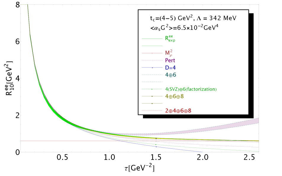
It is informative to compare the QCD prediction of ${\cal L}_{0}$ with the one where the complete $e^{+}e^{-}\to I=1$ Hadrons data is used to estimate the spectral integral. This analysis has been done recently in Ref. SNe23 which we show in Fig. 8

One can observe that there is a good agreement with the experimental $e^{+}e^{-}$ data. and the theory prediction using the previous sets of QCD parameters up to $D=6,8$ condensates.

$\diamond~{}$Within MDA, one expects that the ratio of moments provides the mass squared of the $\rho$-meson ground state. We show the analysis versus $\tau$ and for different values of $t_{c}$ in Fig. 9.

The optimal results are obtained for the sets $(\tau,t_{c})$ from (0.5,1.2) to (1.2,3.0) in units of (GeV^-2, GeV²). We obtain:

where the error comes mainly from the value of $t_{c}$ which we have taken in the conservative range from the beginning of $\tau$ stability until the $t_{c}$-one.

$\diamond~{}$One can restrict this range of $t_{c}$ value using the constraint from the first moment of FESR. It reads FESR1 ; FESR2 :

from which we deduce:

$\diamond~{}$One should note that the low value of $t_{c}$ often chosen by many “QCD sum rules practitioners” to reproduce the value of the experimental mass or to extract the mass of the ground state does not coi ncide with the duality constraint from FESR. At the value of $t_{c}$ in Eq. 48, we obtain from the ratio of moments :

$\diamond~{}$From the previous analysis, the ratio of moments reproduces within 10% the experimental meson mass.

$\diamond~{}$The ratio of moments has the advantage to be less sensitive to $\alpha_{s}$ correction than the moment ${\cal L}_{0}$ as the PT correction starts to order $\alpha_{s}^{2}$. It is then expected to be a good place for extracting the QCD condensates. This analysis has been initiated by Ref. LNT and revised recently in Ref. SNe23 . Using as input the value of the gluon condensate obtained from heavy quark sum rules SNparam ; SNREV22 ; SNREV21 given in Eq. 17, one obtains:

References

- (1) V. De Alfaro, S. Fubini, G. Furlan, C. Rossetti, Currents in hadron physics, North Holland Pub. Co. Amsterdam-London (1973).
- (2) S. Weinberg, Phys. Rev. Lett. 18 (1967) 507.
- (3) T. Das, V.S. Mathur, S. Okubo, Phys. Rev. Lett. 19 (1967) 470.
- (4) E.G. Floratos, S. Narison and E. de Rafael, Nucl. Phys. B155 (1979) 155 and references quoted therein.
- (5) S. Narison and E. de Rafael, Nucl. Phys B169 (1980) 253 and references quoted therein..
- (6) S. Narison, Z. Phys. C 22 (1984) 161.
- (7) M.A. Shifman, A.I. Vainshtein, V.I. Zakharov, Nucl. Phys. B147 (1979) 385; ibid, Nucl. Phys. B147 (1979) 448.
- (8) V.I. Zakharov, Int. J. Mod .Phys. A14, (1999) 4865.
- (9) S. Narison, QCD spectral sum rules, World Sci. Lect. Notes Phys. 26 (1989) 1.
- (10) S. Narison, QCD as a theory of hadrons, Cambridge Monogr. Part. Phys. Nucl. Phys. Cosmol. 17. (2004) 1-778 [hep-ph/0205006].
- (11) S. Narison, Phys. Rept. 84 (1982) 263; ibid, Riv. Nuovo Cim. 10N2 (1987) 1.
- (12) L.J. Reinders, H.R. Rubinstein, S. Yazaki, Phys. Reports 127 (1985) 1.
- (13) R.A. Bertlmann, Acta Phys. Austriaca 53, (1981) 305.
- (14) M.A. Shifman, Prog. Theor. Phys. Suppl. 131 (1998)1; P. Colangelo and A. Khodjamirian, hep-ph/0010175; E. de Rafael, hep-ph/9802448; F.J. Yndurain, Monographs in Physics, Springer-Verlag, New York (1999).
- (15) S. Narison,Nucl.Part. Phys. Proc.324-329 (2023) 94; ibid, 258-259 (2015) 189.
- (16) S. Narison, Nucl. Part. Phys. Proc.312-317 (2021) 87; ibid, 300-302 (2018) 153.
- (17) S. Narison, Nucl. Part. Phys. Proc. 309-311 (2020) 135; ibid 270-272 (2016) 143.
- (18) J.S. Bell, R.A. Bertlmann, Nucl. Phys. B177, (1981) 218; ibid, Nucl. Phys. B187, (1981) 285.
- (19) S. Narison, E. de Rafael, Phys. Lett. B103, (1981) 57.
- (20) J. Bijnens, J. Prades, E. de Rafael, Phys. Lett. B348 (1995) 226.
- (21) S. Narison, Phys. Lett. B210 (1988) 238; ibid, Phys. Lett. B337 (1994) 166.
- (22) A.A. Logunov, L.D. Soloviev, A.N. Tavkhelidze, Phys. Lett. B24 (1967) 181.
- (23) J.J. Sakurai, Phys. Lett. B46 (1973) 207.
- (24) K.G. Chetyrkin, N.V. Krasnikov, A.N. Tavkhelidze, Phys. Lett. B76 (1978) 83.
- (25) A.L. Kataev, N.V. Krasnikov, A.A. Pivovarov, Phys. Lett. B123 (1983) 93.
- (26) S.G. Gorishnii, A.L. Kataev, S.A. Larin, Phys. Lett. B135 (1984) 457.
- (27) R.A. Bertlmann, G. Launer and E. de Rafael, Nucl. Phys. B250, (1985) 61.
- (28) R.A. Bertlmann, C.A. Dominguez, M. Loewe, M. Perrottet and E. de Rafael, Z. Phys. C39 (1988) 231.
- (29) M. Gell-Mann, R.J. Oakes, B. Renner, Phys. Rev. 175 (1968) 2195.
- (30) H.G. Dosch, S. Narison, Phys. Lett. B417 (1998) 173.
- (31) S. Narison, Int. J. Mod. Phys. A33 (2018) no. 10, 185004; Addendum: Int. J. Mod. Phys. A33 (2018) no.10, 1850045.
- (32) S. Narison, R. Tarrach, Phys. Lett. B125 (1983) 217.
- (33) B.L. Ioffe, Prog. Part. Nucl. Phys. 56 (2006) 232; ibid, B188 (1981) 317; ibid, B191 (1981) 591.
- (34) H.G. Dosch, Non-Perturbative Methods (Montpellier 1985); Y. Chung et al.Z. Phys. C25 (1984) 151; H.G. Dosch, M. Jamin, S. Narison, Phys. Lett. B220 (1989) 251.
- (35) A.A. Ovchinnikov, A.A. Pivovarov, Yad. Fiz. 48 (1988) 1135.
- (36) S. Narison, Phys. Lett. B605 (2005) 319.
- (37) S. Narison, Phys. Lett. B673 (2009) 30.
- (38) G. Launer, S. Narison, R. Tarrach, Z. Phys. C26 (1984) 433.
- (39) C.A. Dominguez, J. Sola, Z. Phys. C40 (1988) 63.
- (40) S. Narison, Phys. Lett. B300 (1993) 293; ibid B361 (1995) 121.
- (41) S. Narison, Phys. Lett. B693 (2010) 559, erratum ibid, B705 (2011) 544; ibid, B706 (2012) 412; ibid, B707 (2012) 259.
- (42) S.N. Nikolaev, A.V. Radyushkin, Phys. Lett. B124 (1983) 243.
- (43) T. Schafer, E.V. Shuryak, Rev. Mod. Phys. 70 (1998) 323.
- (44) B.L. Ioffe, A.V. Samsonov, Phys. At. Nucl. 63 (2000) 1448.
- (45) A. Di Giacomo, Non-pertubative Methods, ed. Narison, World Scientific (1985); A. Di Giacomo, G.C. Rossi, Phys. Lett. B100 (1981) 481; M. D’Elia, A. Di Giacomo, E. Meggiolaro, Phys. Lett. B408 (1997) 315.
- (46) S. Narison, arXiv : 2306.14639 [hep-ph] (2023).
- (47) S. Narison, Phys. Lett. B707 (2012) 259.
- (48) S. Narison, Phys. Lett. B718 (2013) 1321; ibid, Nucl. Phys. (Proc.Suppl.) 234 (2013) 187.
- (49) R.M. Albuquerque, S. Narison, D. Rabetiarivony, arXiv : 2301.08199 (2023).
- (50) S. Narison, Phys. Lett. B738 (2014) 346 and references therein.
- (51) K.G. Chetyrkin, J.H. Kühn and M. Steinhauser,Comput. Phys. Comm 133 (2000) 43 and references therein.
- (52) L. Lellouch, E. de Rafael, J. Taron, Phys.Lett. B414(1997)195; C.A. Dominguez, E. de Rafael, Annals Phys. 174 (1987) 372; J. Bijnens, J. Prades, E. de Rafael, Phys. Lett. B348 (1995), 226.
- (53) S. Aoki et al., arXiv:1310.8555 [hep-lat] (2013).
- (54) M.S.A. Alam Khan, arXiv: 2306.10266 [hep-ph] (2023).
- (55) R.L. Workman et al. (Particle Data Group), Prog. Theor. Exp. Phys. 2022 (2022) 083C01.