\patchcmd

\theparentequation\theparentequation.

Landau’s constant related to the classical zero free region of Riemann zeta function.

Your Document Title

Landau’s constant related to a zero free region of Riemann zeta function

1 Introduction

The Riemann zeta function, denoted as $\zeta(s)$ where $s=\sigma+it$ , is a fundamental object in analytic number theory, with significant applications in fields such as matrix theory and physics. It is initially defined for $\sigma>1$ by the series:

\zeta(s)=\sum_{n=1}^{\infty}\frac{1}{n^{s}},

which converges absolutely in this region. However, for $\sigma\leq 1$ , the series diverges. To address this, $\zeta(s)$ admits an analytic continuation to the entire complex plane, except for a simple pole at $s=1$ . The continuation is expressed as:

\zeta(s)=\frac{\pi^{\frac{s}{2}}}{\Gamma\left(\frac{s}{2}\right)}\left(-\frac{1}{s}-\frac{1}{1-s}+\int_{1}^{\infty}\sum_{n=-1}^{\infty}e^{-\pi n^{2}x}\left(x^{s/2-1}+x^{(1-s)/2-1}\right)dx\right).

where $\Gamma(s)$ is the Gamma function.

The zeros of the Riemann zeta function are critical in understanding the distribution of prime numbers. These zeros are classified into trivial zeros, occurring at the negative even integers $s=-2,-4,-6,\ldots$ , and nontrivial zeros, which lie within the critical strip $0<\sigma<1$ . The Riemann Hypothesis conjectures that all nontrivial zeros have a real part $\displaystyle{}\sigma=\frac{1}{2}$ . For further proofs and theoretical background on the Riemann zeta function, one can refer to Apostol [Apo76].

To study the behavior of nontrivial zeros of the Riemann zeta function, the zero-free region of the Riemann zeta function was first established by de la Vallée Poussin [dlVP00] in 1899. The zero-free region is an area in the critical strip where the Riemann zeta function does not vanish. The classical zero-free region has the form:

\sigma>1-\frac{1}{R\log|t|},

where $R$ is a positive constant. In this region, $\zeta(s)\neq 0$ .

Establishing such regions is crucial, as it directly influences the understanding of the distribution of prime numbers. The prime number counting function

\pi(x)=\sum_{p\leq x}1,

counts the number of primes less than $x$ . Landau [vL08] proved that for any $\rho>R$ :

\pi(x)=\int_{2}^{x}\frac{dy}{\log y}+O\left(x(\log x)^{-1/2}e^{-\sqrt{\log x/\rho}}\right).

A smaller $R$ will give a larger zero-free region and a smaller error term in the prime number counting function. Efforts to enlarge the zero-free region have driven researchers to reduce the constant $R$ using various techniques. These refinements improve the approximation of the prime number counting function and yield deeper insights into the zeta function’s zeros. Table 1 summarizes key results in reducing the $R$ constant.

Year	Author	$R$
1899	de la Vallée Poussin [dlVP00]	30.47
1962	Rosser, Schoenfeld [SRS62]	17.52
1970	Stechkin [Ste70]	9.65
1975	Rosser, Schoenfeld [RS75]	9.65
2002	Ford [For02]	8.46
2005	Kadiri [Kad05]	5.69
2022	Mossinghoff, Trudgian, Yang [MTY22]	5.56

Table 1: Values of the

R

constant determined by existing studies.

All of this work has employed a very special type of trigonometric polynomial. Given a positive integer $n\geq 2$ , let $C_{n}$ denotes the set of cosine polynomials:

f(\phi)=\sum_{k=0}^{n}a_{k}\cos(k\phi),

with the following properties:

A.1

All the coefficients are nonnegative and real.
A.2

The coefficient $a_{1}>a_{0}>0$ .
A.3

$f(\phi)\geq 0$ for all real $\phi$ .

Then, the real valued functional $v:C_{n}\to\mathbb{R}$ is defined by:

v(f)=\frac{f(0)-a_{0}}{(\sqrt{a_{1}}-\sqrt{a_{0}})^{2}}.

Landau [vL08] demonstrated that for any $f\in C_{n}$ , one can take:

R=\frac{v(f)}{2},

in the classical zero-free region, ensuring $\zeta(s)\neq 0$ in this region.

Naturally, the goal to enlarge the zero-free region and pursuits the smaller $R$ leads to the following problems.

Problem 1.1.

What is the exact value of

V_{n}=\inf_{f\in C_{n}}\frac{f(0)-a_{0}}{(\sqrt{a_{1}}-\sqrt{a_{0}})^{2}},

and

V=\inf_{n\geq 2}V_{n}.

The problems to find the value of $V$ were studied by Westphal [Wes38], Stechkin [Ste70], Rosser and Schoenfeld [SRS62, RS75], French [Fre66], Kondrat’ev [Kon77, AK90], Reztsov [Rez86], Arestov [AK90, Are92], Mossinghoff and Trudgian [MT14]. Most of the works are dedicated to estimating the upper and lower bounds of $V$ . As of now, the best two-sided estimates for $V$ are:

34.468305<V<34.503586.

The exact value of $V_{n}$ is known only for $n=2,3,4,5,6$ .

To determine the exact value of $V_{2}$ , French [Fre66] substituted $x=\cos\phi$ and expressed every cosine polynomial in $C_{2}$ in the form:

h(x)=(1-a_{2})+a_{1}x+2a_{2}x^{2},

which satisfies the condition $h(x)\geq 0$ for all $x\in[-1,1]$ . French classified the polynomial in two classes based on the global minimum point $(x_{0},h(x_{0}))$ of $h(x)$ . The first class is when $x_{0}\in[-1,1]$ and the second class is when $x_{0}\not\in[-1,1]$ . Then, French calculated the minimum value of $v(f)$ can be attained in two different classes, the smaller number being the exact value of $V_{2}$ .

On the other hand, Arestov use the following properties of nonnegative trigonometric polynomials to evaluate the exact value of $V_{n}$ for $n=3,4,5,6$ . Firstly, he noticed that for any trigonometric polynomial $f_{n}\in C_{n}$ , the Fejér inequality [PS78] holds:

\displaystyle a_{1}(f)\leq A(n)a_{0}(f),\quad A(n)=2\cos\frac{\pi}{n+2}.

(1.1)

Secondly, for any $f\in C_{n}$ and positive number $k$ , one has $v(kf)=v(f)$ . By using the homogeneity of $v(f)$ and Fejér inequality, one can change the problem of finding $V_{n}$ to become:

\displaystyle V_{n}=\inf_{a\in(1,A(n)]}\frac{\chi_{n}(a)}{(\sqrt{a}-1)^{2}},

(1.2)

where $\chi_{n}(a)$ is defined as:

\chi_{n}(a)=\inf\{f(0)-1\mid f(\phi)\in C_{n},a_{0}(f)=1\text{ and }a_{1}(f)=a\}.

Arestov [Are92] used some inequalities of nonnegative trigonometric polynomials to find the exact value of $\chi_{n}(a)$ on some specific intervals. This enabled him to calculate the exact value of $V_{n}$ for $n=3,4,5,6.$ The values of $V_{n}$ for $n=2,3,4,5,6$ are summarized in Table 2.

n	Author	$V_{n}$
2	French [Fre66]	53.1390720
3	Arestov [Are92]	36.9199911
4	Arestov [Are92]	34.8992259
5	Arestov [Are92]	34.8992259
6	Arestov [Are92]	34.8992259

Table 2: Values of

V_{n}

as determined by Arestov.

The goal of this research is to revise the exact values of $V_{n}$ for $n=2,3,4,5,6$ and find the exact values of $V_{n}$ for $n=7,8$ . In Section 2, the exact values of $V_{2}$ and $V_{3}$ will be found by improving French’s method. Instead of classifying the polynomial $h(x)$ by the location of the minimum point, the polynomial will be classified based on the location of its roots.

Sections 3 to Section 8 will be devoted to finding the exact values of $V_{n}$ for $n$ from 4 to 8. By applying the Fejér-Riesz theorem [Fej16], the problem of finding $\chi_{n}(a)$ is transformed into an optimization problem in $\mathbb{R}^{n}$ and then solved using optimization techniques. The techniques and general procedure will be described in Section 3, while the key constraints and result of the optimization problems will be summarized in Section 4 to Section 8. In the last two sections, the following theorems will be presented.

Theorem 1.1: The exact value of $V_{7}$ is

V_{7}=34.6494874.

Theorem 1.2: The exact values of $V_{8}$ is

V_{8}=34.5399155.

This work aims to advance our understanding of the zero-free regions of the Riemann zeta function, thereby contributing to the broader field of analytic number theory and its applications to prime number theory.

2 The exact value of $V_{2}$ and $V_{3}$

2.1 Some properties of function $v(f)$ .

This section is devoted to finding the exact values of $V_{2}$ and $V_{3}$ . Firstly, some useful properties of the function $v(f)$ will be established. These properties will enable a focus on some special forms of polynomials to find the values of $V_{2}$ and $V_{3}$ .

One particularly useful property is the homogeneity of the function $v(f)$ , which implies that for $k>0$ , the function $v$ satisfies $v(kf)=v(f)$ . This property is advantageous because, instead of studying all polynomials $f(\phi)\in C_{n}$ , the focus can be narrowed to polynomials of the form

f(\phi)=1+a\cos\phi+a_{2}\cos 2\phi+\ldots+a_{n}\cos n\phi,

where $\displaystyle{}a\in\left(1,2\cos\frac{\pi}{n+2}\right]$ by Fejér’s Inequality (Equation (1.1)).

To explore next property of $v(f)$ , the following two theorems imply that one only need to consider the cosine polynomial with a minimum of 0 in order to find the exact value of $V_{n}$ .

Theorem 2.1.

Given

f(\phi)=a_{0}+a_{1}\cos\phi+a_{2}\cos 2\phi+\ldots+a_{n}\cos n\phi\in C_{n},

let $m$ be the minimum of $f(\phi)$ when $\phi\in[0,2\pi)$ , then

m<a_{0}.

Proof.

This can be proven easily by considering the integration below,

a_{0}=\frac{1}{2\pi}\int_{0}^{2\pi}f(\phi)d\phi\geq\frac{1}{2\pi}(2\pi)m=m.

The equality holds if and only if $f(\phi)$ is a constant function, which is impossible in the context of this discussion. This completes the proof. ∎

The next theorem states that given a polynomial $f(\phi)\in C_{n}$ with minimum $m>0$ , another polynomial $\bar{f}(\phi)\in C_{n}$ with minimum 0 can always be found such that $v(f)>v(\bar{f})$ . This clearly implies $v(f)>V_{n}$ , thus $f(\phi)$ is not a candidate for the infimum.

Theorem 2.2.

Given $f(\phi)\in C_{n}$ with minimum $m>0$ , let

\bar{f}(\phi)=f(\phi)-m.

Then $\bar{f}(\phi)\in C_{n}$ and

v(f)>v(\bar{f}).

Proof.

To prove $\bar{f}(\phi)\in C_{n}$ , note that $a_{0}(\bar{f})=a_{0}(f)-m>0$ by Theorem 2.1. Moreover, it holds that

a_{1}(\bar{f})=a_{1}(f)>a_{0}(f)>a_{0}(\bar{f}).

Lastly,

	$\displaystyle v(\bar{f})$	$\displaystyle=\frac{a_{1}(f)+a_{2}(f)+a_{3}(f)+\ldots+a_{n}(f)}{\left(\sqrt{a_{1}(f)}-\sqrt{a_{0}(f)-m}\right)^{2}}$
		$\displaystyle<\frac{a_{1}(f)+a_{2}(f)+a_{3}(f)+\ldots+a_{n}(f)}{\left(\sqrt{a_{1}(f)}-\sqrt{a_{0}(f)}\right)^{2}}$
		$\displaystyle=v(f).$

This completes the proof.

∎

With the previous theorems, it is established that only cosine polynomials with a minimum of 0 need to be considered in the process of evaluating exact value of $V_{n}$ . The next step is to analyze the properties of the root of these cosine polynomials.

Theorem 2.3.

Given a non-negative cosine polynomial $f(\phi)\in C_{n}$ with minimum 0 , where

f(\phi)=a_{0}+a_{1}\cos\phi+a_{2}\cos 2\phi+\ldots+a_{n}\cos n\phi,

then $f(\phi)$ must have at least one root $\phi_{0}$ in the interval $[0,2\pi)$ , and it must satisfy one of the following:

a.

The root $\phi_{0}=\pi$ (or $\cos\phi_{0}=-1$ ).
b.

The root must have even order.

This will imply if $\phi_{0}\neq\pi$ (or $\cos\phi_{0}\neq-1$ ), then it must have even order.

Proof.

By substituting $x=\cos\phi,f(\phi)$ can be transformed into the polynomial form:

h(x)=b_{n}x^{n}+\ldots+b_{2}x^{2}+b_{1}x+b_{0},

where the fact that $f(\phi)$ is non-negative and has a minimum of zero implies $h(x)$ is non-negative in the interval $[-1,1]$ and has at least one root in this interval. If the root of $h(x)$ lies within the interval $(-1,1)$ , it must be of even order, as it also functions as a local minimum point for the function $h(x)$ . In other words, only $x=1$ and $x=-1$ can serve as the root in $[-1,1]$ with odd order.

However, $x=1$ cannot serve as the root of $h(x)$ . This is shown by contradiction. If $h(x)$ has $x=1$ as its root, then $f(\phi)$ can be expressed as

f(\phi)=(\cos\phi-1)g_{n-1}(\phi),

where $g_{n-1}(\phi)$ is a nonnegative trigonometric polynomial with degree $n-1$ , this implies $f(0)=0$ . This will never happen since

f(0)=a_{n}+a_{n-1}+\ldots+a_{2}+a_{1}+a_{0}>0.

This completes the proof. ∎

Finally, to find the exact value of $V_{n}$ , it is enough to consider only cosine polynomials with at least one double root. Using a similar method in the proof of Theorem 2.2, it will be shown that given any cosine polynomial $f(\phi)\in C_{n}$ which does not have a double root, a polynomial $\bar{f}(\phi)\in C_{n}$ with a double root can always be found such that $v(f)>v(\bar{f})$ . This implies $f(\phi)$ is not a candidate for attaining infimum.

The exact formula of $\bar{f}(\phi)$ will be provided in Theorem 2.4, and subsequently, in Theorem 2.5, it will be shown that $\bar{f}$ satisfies the rquire properties.

Theorem 2.4.

Given

		$\displaystyle f(\phi)=(\cos\phi+1)\left(f_{n-1}(\phi)+m\right),$
		$\displaystyle\bar{f}(\phi)=(\cos\phi+1)f_{n-1}(\phi),$

where $m>0$ and $f_{n-1}(\phi)$ is an $(n-1)$ -degree nonnegative trigonometric polynomial with minimum 0, then

a.

The polynomial $f(\phi)\in C_{n}$ if and only if $\bar{f}(\phi)\in C_{n}$ .
b.

If $f(\phi)\in C_{n}$ , then

$v(f(\phi))>v(\bar{f}(\phi)).$

Proof.

First of all, one can easily see that both $f(\phi)$ and $\bar{f}(\phi)$ satisfy the nonnegative condition. To prove the statement (a), note that

f(\phi)=\bar{f}(\phi)+m\cos\phi+m.

If $f(\phi)\in C_{n}$ , then all the coefficients of $\bar{f}(\phi)$ should also be nonnegative since $a_{k}(\bar{f})\geq a_{k}(f)$ for $k=1,2,\ldots,n$ . Lastly, it is also easy to check $a_{1}(\bar{f})-a_{0}(\bar{f})=a_{1}(f)-$ $a_{0}(f)>0$ , which implies $\bar{f}(\phi)\in C_{n}$ .

Conversely, assume that $\bar{f}(\phi)\in C_{n}$ . It will be shown that $f(\phi)\in C_{n}$ . Firstly, by Theorem 2.1, $a_{0}(f)>0$ . The fact that $a_{1}(\bar{f})-a_{0}(\bar{f})=a_{1}(f)-a_{0}(f)>0$ implies

a_{1}(f)>a_{0}(f)>0

Moreover, $a_{n}(f)\geq 0$ for $n\geq 2$ can be deduced by the fact $a_{n}(f)=a_{n}(\bar{f})\geq 0$ for $n\geq 2$ .

To prove the second statement, just note that for $m>0$ , it holds that

\left(\sqrt{a_{1}(\bar{f})+m}-\sqrt{a_{0}(\bar{f})+m}\right)^{2}<\left(\sqrt{a_{1}(\bar{f})}-\sqrt{a_{0}(\bar{f})}\right)^{2}

This implies

v(f(\phi))=\frac{a_{3}(\bar{f})+a_{2}(\bar{f})+a_{1}(\bar{f})+m}{\left(\sqrt{a_{1}(\bar{f})+m}-\sqrt{a_{0}(\bar{f})+m}\right)^{2}}>\frac{a_{3}(\bar{f})+a_{2}(\bar{f})+a_{1}(\bar{f})}{\left(\sqrt{a_{1}(\bar{f})}-\sqrt{a_{0}(\bar{f})}\right)^{2}}=v(\bar{f}(\phi))

This completes the proof.

∎

To complete the discussion of this subsection, the final theorem will be proven, which shows the $\bar{f}(\phi)$ has at least one double root.

Theorem 2.5.

Given $f(\phi)\in C_{n}$ which does not have a double root, it is always possible to find another $\bar{f}(\phi)\in C_{n}$ with at least one double root such that

v(f)>v(\bar{f}).

Proof.

One can always use Theorem 2.2 to replace $f(\phi)$ with a cosine polynomial that has at least one root. Thus, without loss of generality, only the cosine polynomial with at least a single root in the interval $[0,2\pi)$ needs to be considered. By Theorem 2.3, the cosine polynomial $f(\phi)$ must have the form

f(\phi)=(\cos\phi+1)\left(f_{n-1}(\phi)+m\right)

where $f_{n-1}(\phi)$ is a $(n-1)$ -degree nonnegative trigonometric polynomial with minimum 0 and $m>0$ . Then, let

\bar{f}(\phi)=(\cos\phi+1)f_{n-1}(\phi)

Theorem 2.4 implies that $\bar{f}(\phi)\in C_{n}$ and $v(f)>v(\bar{f})$ . The last thing to prove is that $\bar{f}(\phi)$ has at least one double root. Let $x=\cos\phi$ and transform $\bar{f}(\phi)$ to $\bar{h}(x)$ , that is $\bar{h}(\cos\phi)=\bar{f}(\phi)$ . Then

\bar{h}(x)=(x+1)h_{n-1}(x)

where $h_{n-1}(x)$ is nonnegative in the interval $[-1,1]$ , and the minimum in this interval is 0 . The polynomial $h_{n-1}(x)$ has a zero in the interval $[-1,1]$ . If the zero is in $(-1,1)$ , then it is a double zero. If the zero is $x=-1$ , then $\bar{h}(x)$ has a double zero at $x=-1$ . If the zero is $x=1,thenf(0)=h(1)=0$ implies $\bar{f}(\phi)=\bar{h}(\cos\phi)\notin C_{n}$ , which implies $f(\phi)\notin C_{n}$ , which is a contradiction. The proof is complete. ∎

As a summary, to find the exact value of $V_{n}$ , it is only necessary to consider the cosine polynomials in the following set.

Definition 2.1.

The set $C_{n}^{0}$ is the set containing all degree $n$ cosine polynomials

f(\phi)=a_{0}+a_{1}\cos\phi+a_{2}\cos 2\phi+\ldots+a_{n}\cos n\phi

which satisfy the following three conditions:

B.1

The function $f(\phi)$ is nonnegative and has a double root.
B.2

All the coefficients are nonnegative.
B.3

The coefficient $a_{1}>a_{0}>0$ .

By focusing on the special forms of polynomials and utilizing the properties discussed in the theorems above, the process of finding the exact values of $V_{2}$ and $V_{3}$ can be simplified.

2.2 Exact value of $V_{2}$ .

To find the exact value of $V_{2}$ , Theorem 2.5 and Definition 2.1 imply that it is only necessary to consider the cosine polynomial with double root. Moreover, the homogeneity of $v(f)$ implies it is enough to consider cosine polynomial with the form

f(\phi)=(\cos\phi+\alpha)^{2},

where $\alpha\in[-1,1]$ . However, one still need to check when $f(\phi)\in C_{2}^{0}$ .

Theorem 2.6.

For $-1\leq\alpha\leq 1$ , the polynomial

f(\phi)=(\cos\phi+\alpha)^{2}\in C_{2}^{0}

if and only if $\displaystyle{}1-\frac{1}{\sqrt{2}}<\alpha<1$ .

Proof.

The nonnegative property of $f(\phi)$ is obvious. Expanding $f(\phi)$ , we have

f(\phi)=\cos^{2}\phi+2\alpha\cos\phi+\alpha^{2}=\cos 2\phi+2\alpha\cos\phi+\alpha^{2}+1.

Then $f(\phi)\in C_{2}^{0}$ if and only if

2\alpha>\alpha^{2}+\frac{1}{2}.

Rearranging, we get

\alpha^{2}-2\alpha+\frac{1}{2}<0,

which simplifies to

1-\frac{1}{\sqrt{2}}<\alpha<1.

This completes the proof. ∎

The next theorem presents the exact value of $V_{2}$ and the cosine polynomial $f(\phi)\in C_{2}$ such that $v(f)=V_{2}$ .

Theorem 2.7.

The exact value of $V_{2}$ is

V_{2}=53.1390720,

which can be obtained by considering

f(\phi)=(\cos\phi+0.7415574)^{2}.

Proof.

By Theorem 2.6, only the polynomials in the following form need to be considered:

f(\phi)=(\cos\phi+\alpha)^{2},

where $\displaystyle{}1-\frac{1}{\sqrt{2}}<\alpha<1$ . In this case,

f(\phi)=\cos^{2}\phi+2\alpha\cos\phi+\alpha^{2}=\frac{1}{2}\cos 2\phi+2\alpha\cos\phi+\alpha^{2}+\frac{1}{2},

thus

v(f(\phi))=\frac{0.5+2\alpha}{(\sqrt{2\alpha}-\sqrt{\alpha^{2}+0.5})^{2}}.

This function is continuous in the interval $\displaystyle{}\alpha\in\left(1-\frac{1}{\sqrt{2}},1\right)$ . Using Matlab to conduct a golden section search, the minimum is found to be 53.1390720 (see Figure 1),

Refer to caption — Figure 1: Graph of $v(f(\phi))$ .

which can be obtained by considering

f(\phi)=(\cos\phi+0.7415574)^{2}.

This completes the proof. ∎

2.3 Exact value of $V_{3}$ .

This subsection will be devoted to finding the exact value of $V_{3}$ . To find the exact value of $V_{3}$ , Theorem 2.5 and Definition 2.1 imply that it is only necessary to consider the cosine polynomial with double root. Moreover, the homogeneity of $v(f)$ implies it is enough to consider cosine polynomial with the form

f(\phi)=(\cos\phi+\alpha)^{2}(\cos\phi+\beta),

where $\alpha\in[-1,1]$ and $\beta\geq 1$ .

Our next goal is to identify all the polynomials in this form that belong to $C_{3}^{0}$ .

Theorem 2.8.

For $-1\leq\alpha\leq 1$ and $\beta\geq 1$ , the cosine polynomial

f(\phi)=(\cos\phi+\alpha)^{2}(\cos\phi+\beta)

belongs to $C_{3}^{0}$ if and only if

a.

$\displaystyle{}\alpha\geq 1-\frac{1}{\sqrt{2}}$ , or
b.

$\displaystyle{}-\frac{1}{4}<\alpha<1-\frac{1}{\sqrt{2}}$ and $\displaystyle{}\beta\in\left[1,1+\frac{4\alpha+1}{4\alpha^{2}-8\alpha+2}\right)$ .

Proof.

To check that a cosine polynomial belongs to $C_{3}^{0}$ , we need to check all the conditions stated in Definition 2.1. It is obvious that for every $\alpha\in[-1,1]$ and $\beta\geq 1$ , the polynomial $f(\phi)$ is nonnegative and has a double root. Next, expanding $f(\phi)$ , we obtain

f(\phi)=\cos 3\phi+(2\beta+4\alpha)\cos 2\phi+(4\alpha^{2}+8\alpha\beta+3)\cos\phi+(4\alpha^{2}\beta+4\alpha+2\beta).

To ensure $f(\phi)$ satisfies $a_{1}>a_{0}$ , consider the inequality:

4\alpha^{2}+8\alpha\beta+3>4\alpha^{2}\beta+4\alpha+2\beta.

Rearranging, one get

4\alpha^{2}-4\alpha+3>\beta(4\alpha^{2}-8\alpha+2).

It is obvious that $4\alpha^{2}-4\alpha+3=(2\alpha-1)^{2}+2$ is positive. When $\displaystyle{}\alpha\geq 1-\frac{1}{\sqrt{2}}$ , we have $\displaystyle{}4\alpha^{2}-8\alpha+2\leq 0$ , thus the inequality holds. When $\displaystyle{}\alpha<1-\frac{1}{\sqrt{2}}$ , one needs to have

\beta<\frac{4\alpha^{2}-4\alpha+3}{4\alpha^{2}-8\alpha+2}=1+\frac{4\alpha+1}{4\alpha^{2}-8\alpha+2}.

Thus, when $\displaystyle{}\alpha\leq-\frac{1}{4}$ , one has $\displaystyle{}\beta<1$ , which contradicts the assumption. When $\displaystyle{}-\frac{1}{4}<\alpha<1-\frac{1}{\sqrt{2}}$ , one has

\beta\in\left[1,1+\frac{4\alpha+1}{4\alpha^{2}-8\alpha+2}\right).

One can also check that when $\displaystyle{}\alpha>-\frac{1}{4}$ , we have $a_{2}=4\alpha+2\beta>0$ and $a_{0}=4\alpha^{2}\beta+4\alpha+2\beta>0$ . This shows the polynomial $f(\phi)$ is in $C_{3}^{0}$ . This completes the proof. ∎

Next, it will be demonstrated that in order to determine the exact value of $V_{3}$ , it suffices to consider degree 3 polynomials of the form

f(\phi)=(\cos\phi+\alpha)^{2}(\cos\phi+1),

where $\displaystyle{}\alpha\in\left(-\frac{1}{4},1\right]$ . The same strategy as used in the proof of Theorem 2.2 will be applied here. Given a cosine polynomial $f(\phi)$ in the form

f(\phi)=(\cos\phi+\alpha)^{2}(\cos\phi+\beta),

where $\displaystyle{}\alpha\in\left(-\frac{1}{4},1\right]$ and $\beta>1$ , another polynomial

\bar{f}(\phi)=(\cos\phi+\alpha)^{2}(\cos\phi+1)

can be constructed and yields a better result, implying that $v(f)>v(\bar{f})$ . Consequently, $f$ is not a candidate for the infimum.

To establish this result, we first require some preliminary lemmas. Three of the following lemmas provide simple inequalities that will be used to compare the values of $v(f)$ and $v(\bar{f})$ . Readers may choose to skip ahead to Theorem 2.12 and return to these lemmas when the inequalities are needed. For a smoother reading experience, the proofs of Lemma 2.9, Lemma 2.10 and Lemma 2.11 are presented in the Appendix A.

Lemma 2.9.

Given four positive real numbers $a,b,\Delta a,\Delta b$ , if

\frac{\Delta a}{\Delta b}>\frac{a}{b},

then

\frac{a+\Delta a}{b+\Delta b}>\frac{a}{b}.

Lemma 2.10.

Given five positive real numbers $a_{1},a_{2},b_{1},b_{2},k$ , if

\frac{a_{1}}{b_{1}}>k\quad\text{and}\quad\frac{a_{2}}{b_{2}}>k,

then

\frac{a_{1}+a_{2}}{b_{1}+b_{2}}>k.

Lemma 2.11.

Given four positive real numbers $a,b,\Delta a,\Delta b$ , then

\sqrt{(a+\Delta a)(b+\Delta b)}\geq\sqrt{ab}+\sqrt{\Delta a\Delta b},

equality holds when $a\Delta b=b\Delta a.$

The following theorem compares the value of $v(f)$ and $v(\bar{f})$ , and implies that we only need to consider the cosine polynomial in the form of

\bar{f}(\phi)=(\cos\phi+\alpha)^{2}(\cos\phi+1)

in order to find the exact value of $V_{3}$ .

Theorem 2.12.

Given a cosine polynomial in $C_{3}^{0}$ of the form

f(\phi)=(\cos\phi+\alpha)^{2}(\cos\phi+\beta),

let

\bar{f}(\phi)=(\cos\phi+\alpha)^{2}(\cos\phi+1).

Then $\bar{f}(\phi)\in C_{3}^{0}$ and

v(f(\phi))>v(\bar{f}(\phi)).

Proof.

When $\displaystyle{}\alpha\in\left(-\frac{1}{4},1-\frac{1}{\sqrt{2}}\right]$ , it will be shown that $v(f(\phi))$ increases as $\beta$ increases by proving $\displaystyle{}\frac{\partial v(f)}{\partial\beta}>0$ for $\beta\geq 1$ . Expanding $f(\phi)$ , we have

f(\phi)=\cos 3\phi+(2\beta+4\alpha)\cos 2\phi+(4\alpha^{2}+8\alpha\beta+3)\cos\phi+(4\alpha^{2}\beta+4\alpha+2\beta),

thus

v(f(\phi))=\frac{4\alpha^{2}+8\alpha\beta+4\alpha+2\beta+4}{\left(\sqrt{4\alpha^{2}+8\alpha\beta+3}-\sqrt{4\alpha^{2}\beta+4\alpha+2\beta}\right)^{2}}.

To show $\displaystyle{}\frac{\partial v(f)}{\partial\beta}$ is positive, it is enough to prove

	$\displaystyle\bar{v}$	$\displaystyle=\left(\sqrt{4\alpha^{2}+8\alpha\beta+3}-\sqrt{4\alpha^{2}\beta+4\alpha+2\beta}\right)(8\alpha+2)$
		$\displaystyle-\left(4\alpha^{2}+8\alpha\beta+4\alpha+2\beta+4\right)\left(\frac{8\alpha}{\sqrt{4\alpha^{2}+8\alpha\beta+3}}-\frac{4\alpha^{2}+2}{\sqrt{4\alpha^{2}\beta+4\alpha+2\beta}}\right)>0.$

When $\displaystyle{}\alpha\in\left(-\frac{1}{4},1-\frac{1}{\sqrt{2}}\right]$ , we have $4\alpha^{2}+2\geq 8\alpha$ , and thus

\frac{8\alpha}{\sqrt{4\alpha^{2}+8\alpha\beta+3}}\leq\frac{4\alpha^{2}+2}{\sqrt{4\alpha^{2}+8\alpha\beta+3}}\leq\frac{4\alpha^{2}+2}{\sqrt{4\alpha^{2}\beta+4\alpha+2\beta}}.

This implies

\frac{8\alpha}{\sqrt{4\alpha^{2}+8\alpha\beta+3}}-\frac{4\alpha^{2}+2}{\sqrt{4\alpha^{2}\beta+4\alpha+2\beta}}\leq 0,

and thus $\bar{v}>0$ since we know that $\sqrt{a_{1}}-\sqrt{a_{0}}>0$ , $8\alpha+2>0$ , and $a_{3}+a_{2}+a_{1}>0$ .

For the case where $\displaystyle{}\alpha\geq 1-\frac{1}{\sqrt{2}}$ , we want to prove that

v(f(\phi))>v(\bar{f}(\phi)).

If we write $f(\phi)=(\cos\phi+\alpha)^{2}(\cos\phi+1+m)$ , where $m>0$ , then the statement we want to prove turns to

		$\displaystyle\frac{4\alpha^{2}+12\alpha+6+m(8\alpha+2)}{\left(\sqrt{4\alpha^{2}+8\alpha+3+8\alpha m}-\sqrt{4\alpha^{2}+4\alpha+2+2m+4\alpha^{2}m}\right)^{2}}$
	$\displaystyle>$	$\displaystyle\frac{4\alpha^{2}+12\alpha+6}{\left(\sqrt{4\alpha^{2}+8\alpha+3}-\sqrt{4\alpha^{2}+4\alpha+2}\right)^{2}}.$

Now, let

		$\displaystyle\Delta_{1}=(8\alpha+2)m,$
		$\displaystyle\Delta_{2}=\left(\sqrt{a_{1}+8\alpha m}-\sqrt{a_{0}+(4\alpha^{2}+2)m}\right)^{2}-\left(\sqrt{a_{1}}-\sqrt{a_{0}}\right)^{2},$

where $a_{1}=4\alpha^{2}+8\alpha+3$ and $a_{0}=4\alpha^{2}+4\alpha+2$ . By Lemma 2.11, one can show that

	$\displaystyle\Delta_{2}$	$\displaystyle=\left(4\alpha^{2}+8\alpha+2\right)m-2\sqrt{\left(a_{1}+8\alpha m\right)\left(a_{0}+\left(4\alpha^{2}+2\right)m\right)}+2\sqrt{a_{1}a_{0}}$
		$\displaystyle<\left(4\alpha^{2}+8\alpha+2\right)m-2\sqrt{a_{1}a_{0}}-2m\sqrt{8\alpha\left(4\alpha^{2}+2\right)}+2\sqrt{a_{1}a_{0}}$
		$\displaystyle=m\left[4\alpha^{2}+8\alpha+2-2\sqrt{8\alpha\left(4\alpha^{2}+2\right)}\right].$

Using Matlab to conduct a golden section search (see Figure 2), one can check that for $\displaystyle{}\alpha\in\left[1-\frac{1}{\sqrt{2}},1\right]$ ,

\frac{\Delta_{1}}{\Delta_{2}}>\frac{8\alpha+2}{4\alpha^{2}+8\alpha+2-2\sqrt{8\alpha\left(4\alpha^{2}+2\right)}}\geq 53.1390720.

The minimum point can be obtained when $\alpha=0.7415574$ .

Moreover, one can also use the same method (see Figure 3) to check

v(\bar{f}(\phi))=\frac{4\alpha^{2}+12\alpha+6}{\left(\sqrt{4\alpha^{2}+8\alpha+3}-\sqrt{4\alpha^{2}+4\alpha+2}\right)^{2}}\leq 22+\frac{44\sqrt{6}}{5}=43.5555097.

The maximum point can be obtained when $\alpha=1$ . Thus, by Lemma 2.9, we have

v(f(\phi))=\frac{4\alpha^{2}+12\alpha+6+\Delta_{1}}{\left(\sqrt{4\alpha^{2}+8\alpha+3}-\sqrt{4\alpha^{2}+4\alpha+2}\right)^{2}+\Delta_{2}}>v(\bar{f}(\phi)).

This completes the proof. ∎

Finally, the last theorem of this section presents the exact value of $V_{3}$ and identifies the cosine polynomial $f(\phi)\in C_{3}$ such that $v(f)=V_{3}$ .

Theorem 2.13.

The exact value of $V_{3}$ is

V_{3}=36.9199911,

which can be obtained by considering the cosine polynomial

f(\phi)=4(\cos\phi+1)(\cos\phi+0.4384345)^{2}.

Proof.

Theorem 2.8 implies that we only need to consider the cosine polynomial in the form

f(\phi)=4(\cos\phi+\alpha)^{2}(\cos\phi+\beta)

where $\alpha,\beta$ satisfy one of the following:

a.

$\displaystyle{}\alpha\in\left[1-\frac{1}{\sqrt{2}},1\right]$ , or
b.

$\displaystyle{}-\frac{1}{4}<\alpha<1-\frac{1}{\sqrt{2}}$ and $\beta\in\left[1,1+\frac{4\alpha+1}{4\alpha^{2}-8\alpha+2}\right)$ .

Moreover, Theorem 2.12 implies that we need only consider the case where $\beta=1$ . As a result, the polynomial takes the form

f(\phi)=4(\cos\phi+\alpha)^{2}(\cos\phi+1),

where $\displaystyle{}\alpha\in\left(-\frac{1}{4},1\right]$ . Expanding $f(\phi)$ , we obtain

f(\phi)=\cos 3\phi+(4\alpha+2)\cos 2\phi+(4\alpha^{2}+8\alpha+3)\cos\phi+(4\alpha^{2}+4\alpha+2).

In this case, we have

v(f(\phi))=\frac{4\alpha^{2}+12\alpha+6}{\left(\sqrt{4\alpha^{2}+8\alpha+3}-\sqrt{4\alpha^{2}+4\alpha+2}\right)^{2}}.

One can check that this function is continuous in the interval $\displaystyle{}\left(-\frac{1}{4},1\right]$ . Using Matlab to conduct a golden section search (see Figure 4), the minimum is 36.9199911, which can be obtained by considering the cosine polynomial

f(\phi)=4(\cos\phi+1)(\cos\phi+0.4384345)^{2}.

This completes the proof. ∎

3 Methodology

The Fejer-Riesz theorem was first employed by Kondrat’ev [Kon77] to find the upper bound of $V_{8}$ in his paper. This method was later employed by Mossinghoff and Trudgian [MT14] to determine the upper bound of $V_{n}$ for $n=8,12,16,\ldots,40$ . The Fejer-Riesz theorem translates the problem of finding the exact value of $V_{n}$ into a minimization problem on $\mathbb{R}^{n}$ , subject to certain conditions. The statement of the Fejer-Riesz theorem is presented as follows:

Theorem 3.1 (Fejer-Riesz theorem).

[Fej16] Let $\displaystyle g(\phi)=\sum_{k=0}^{n}b_{k}\cos k\phi$ be a trigonometric polynomial with real coefficients, which is nonnegative for every real $\phi$ and $b_{n}\neq 0$ . Then, there exist real numbers $\alpha_{0},\alpha_{1},\alpha_{2},\ldots,\alpha_{n}$ such that

g(\phi)=\left|\sum_{k=0}^{n}\alpha_{k}e^{ik\phi}\right|^{2}.

Moreover, we also have

b_{0}=\sum_{k=0}^{n}\alpha_{k}^{2}\quad\text{and}\quad b_{j}=\sum_{k=0}^{n-j}\alpha_{k}\alpha_{k+j}.

Now, given any cosine polynomial in $C_{n}$ ,

f(\phi)=1+a\cos\phi+\sum_{k=2}^{n}a_{k}\cos k\phi,

the Fejer-Riesz theorem states that we can find real numbers $x_{0},x_{1},x_{2},\ldots,x_{n}$ such that

f(\phi)=\left|\sum_{k=0}^{n}x_{k}e^{ik\phi}\right|^{2},

with the following conditions:

	$\displaystyle x_{0}^{2}+x_{1}^{2}+x_{2}^{2}+\ldots+x_{n}^{2}=1,$
	$\displaystyle 2(x_{0}x_{1}+x_{1}x_{2}+\ldots+x_{n-1}x_{n})=a,$
	$\displaystyle 2(x_{0}x_{k}+x_{1}x_{k-1}+\ldots+x_{n-k}x_{n})\geq 0,$

for $2\leq k\leq n$ .

By observing that

f(0)=(x_{0}+x_{1}+\ldots+x_{n})^{2}-1,

the problem of finding the exact value of $\chi_{n}(a)$ in Equation (1.2) is equivalent to the following minimization problem, which we call Problem $P_{1}$ .

Problem 3.1.

The optimization Problem $P_{1}$ is defined as

	$P_{1}$ : Minimize	$\displaystyle F(\mathbf{x})=(x_{0}+x_{1}+\ldots+x_{n})^{2}-1$
	subject to	$\displaystyle H_{1}(\mathbf{x})=x_{0}^{2}+x_{1}^{2}+x_{2}^{2}+\ldots+x_{n}^{2}=1,$
		$\displaystyle H_{2}(\mathbf{x})=2(x_{0}x_{1}+x_{1}x_{2}+\ldots+x_{n-1}x_{n})=a,$
		$\displaystyle G_{1}(\mathbf{x})=2(x_{0}x_{2}+x_{1}x_{3}+\ldots+x_{n-2}x_{n})\geq 0,$
		$\displaystyle G_{2}(\mathbf{x})=2(x_{0}x_{3}+x_{1}x_{4}+\ldots+x_{n-3}x_{n})\geq 0,$
		$\displaystyle\quad\quad\quad\vdots$
		$\displaystyle G_{n-1}(\mathbf{x})=2x_{0}x_{n}\geq 0.$

For Problem $P_{1}$ , we denote the subset of $\mathbb{R}^{n}$ that satisfies all the conditions in the statement of the problem as $S_{1}$ . One can note that if $S_{1}$ is not empty, then it will be a closed set since

\text{S1}=H_{1}^{-1}(\{1\})\cap H_{2}^{-1}(\{a\})\cap\bigcap_{i=1}^{n-1}G_{i}^{-1}([0,\infty)).

Moreover, the condition $H_{1}(\mathbf{x})=1$ implies that $S_{1}$ is bounded, meaning $S_{1}$ is a compact set. Since all the functions $F,H_{i}$ , and $G_{i}$ are continuous, the existence of a global solution is guaranteed by the Weierstrass Extreme Value Theorem.

Theorem 3.2 (Weierstrass Extreme Value Theorem).

[Mun00] Every continuous function on a compact set attains its extreme values on that set.

Applying the Weierstrass Extreme Value Theorem to Problem $P_{1}$ guarantees the existence of a global minimum for $F(\mathbf{x})$ on the set $S_{1}$ .

3.1 Karush-Kuhn-Tucker Method

In order to solve Problem $P_{1}$ , two classical approaches in mathematical optimization will be applied, which are Karush-Kuhn-Tucker conditions and penalty function. The Karush-Kuhn-Tucker conditions are the first derivative tests for a solution to be optimal in nonlinear programming. Given an optimization problem, we call it Problem $P$ .

Problem 3.2.

The optimization Problem $P$ is defined as

\begin{array}[]{ll}\text{ $P$:Minimize }&f(\mathbf{x})\\ \text{ subject to }&g_{i}(\mathbf{x})\leq 0\text{ for }i=1,\ldots,j\\ &h_{i}(\mathbf{x})=0\text{ for }i=1,\ldots,k\\ \end{array}

where $f,g_{1},\ldots,g_{j},h_{1},\ldots,h_{k}$ are all continuous function from $\mathbb{R}^{n}$ to $\mathbb{R}$ .

For Problem $P$ , we denote the feasible regions as $S$ , which is defined as

S=\{{\mathbf{x}}=(x_{1},x_{2},\ldots,x_{n})\in\mathbb{R}^{n}|h_{i}({\mathbf{x}})=0,g_{i}({\mathbf{x}})\leq 0\}.

To guarantee the set $S$ is nonempty, the Slater’s condition will be checked in advance.

Definition 3.1 (Slater’s condition).

[BSS06] The Problem $P$ is said to satisfy Slater’s condition if we can find a vector $\mathbf{x}\in\mathbb{R}^{n}$ such that

g_{1}(\mathbf{x})<0,g_{2}(\mathbf{x})<0,\cdots,g_{m}(\mathbf{x})<0.

The Karush-Kuhn-Tucker conditions are a set of requirements that must be satisfied by the optimal point of an optimization problem.

Theorem 3.3 (Karush-Kuhn-Tucker Necessary Conditions).

[BSS06] Let $f:R^{n}\rightarrow R$ , and $g_{i}:R^{n}\rightarrow R$ for $i=$ $1,\ldots,m$ . Consider Problem ${P}$ , which seeks to minimize $f({\mathbf{x}})$ subject to $g_{i}({\mathbf{x}})\leq 0$ for $i=1,\ldots,j$ and $h_{i}(\mathbf{x})=0$ for $i=1,\ldots,k$ . Suppose $\overline{\mathbf{x}}$ is a solution to this problem, and that $f,g_{i}$ and $h_{i}$ are all differentiable at $\overline{\mathbf{x}}$ . Furthermore, assume the gradients of the constraints, $\nabla g_{i}(\overline{\mathbf{x}})$ , are linearly independent for all $i$ . If $\overline{\mathbf{x}}$ solves Problem $\mathrm{P}$ locally, there exist scalars $u_{i}$ for $i\in I$ such that:

$\displaystyle\nabla f(\overline{\mathbf{x}})+\sum_{i=1}^{j}\lambda_{i}\nabla h_{i}(\mathbf{x})+\sum_{i=1}^{k}u_{i}\nabla g_{i}(\overline{\mathbf{x}})$	$\displaystyle=\mathbf{0}$
$\displaystyle u_{i}g_{i}(\overline{\mathbf{x}})$	$\displaystyle=0$	$\displaystyle\text{ for }i=1,\ldots,m$
$\displaystyle u_{i}$	$\displaystyle\geq 0$	$\displaystyle\text{ for }i=1,\ldots,m.$

For the problem $P_{1}$ (Problem 3.1), since we can guarantee the existence of the optimal solution $\overline{\mathbf{x}}$ , this means we can find scalar $\lambda_{1},\lambda_{2},u_{1},u_{2},\ldots,u_{n-1}$ such that:

$\displaystyle\nabla F(\overline{\mathbf{x}})+\sum_{i=1}^{2}\lambda_{i}\nabla H_{i}(\mathbf{x})+\sum_{i=1}^{n-1}u_{i}\nabla G_{i}(\overline{\mathbf{x}})$	$\displaystyle=\mathbf{0}$
$\displaystyle u_{i}G_{i}(\overline{\mathbf{x}})$	$\displaystyle=0$	$\displaystyle\text{ for }i=1,\ldots,n$
$\displaystyle u_{i}$	$\displaystyle\geq 0$	$\displaystyle\text{ for }i=1,\ldots,n.$

3.2 Penalty Function

The second tool used is the penalty function, which transforms a constrained optimization problem into an unconstrained one. This is done by incorporating the constraints into the objective function through a penalty parameter that penalizes any violation of the constraints.

Consider Problem $P$ again. We can replace Problem $P$ with the following unconstrained problem.

Problem 3.3.

The optimization Problem $P_{2}$ is defined as

	Minimize	$\displaystyle\quad f(\mathbf{x})+\mu\left[\sum_{i=1}^{j}\left(h_{i}(\mathbf{x})\right)^{2}+\sum_{i=1}^{k}\max\{g_{i}(\mathbf{x}),0\}^{2}\right]$
	subject to	$\displaystyle\quad\mu\geq 0.$

For $\mu\geq 0$ , let us denote

\alpha(\mathbf{x})=\sum_{i=1}^{j}\left(h_{i}(\mathbf{x})\right)^{2}+\sum_{i=1}^{k}\max\{g_{i}(\mathbf{x}),0\}^{2},

and

\theta(\mu)=\inf\left\{f(\mathbf{x})+\mu\alpha(\mathbf{x})\right\}.

One can observe that when $\mu$ is a large positive number, any point $\mathbf{x}\in\mathbb{R}^{n}$ that violates the conditions in Problem $P$ will give $\alpha(\mathbf{x})$ a large value, which causes $f(\mathbf{x})+\mu\alpha(\mathbf{x})>\theta(\mu)$ .

The following theorem concludes this subsection, which states that solving Problem $P$ is equivalent to finding the value of

\lim_{\mu\to\infty}\theta(\mu).

Theorem 3.4.

[BSS06] Consider the following problem:

\begin{array}[]{ll}\text{Minimize}&f(\mathbf{x})\\ \text{subject to}&g_{i}(\mathbf{x})\leq 0\text{ for }i=1,\ldots,j\\ &h_{i}(\mathbf{x})=0\text{ for }i=1,\ldots,k\\ \end{array}

where $f,g_{1},\ldots,g_{j},h_{1},\ldots,h_{k}$ are continuous functions on $\mathbb{R}^{n}$ . Suppose that the problem has a feasible solution, and let $\alpha$ be a continuous function defined by

\alpha(\mathbf{x})=\sum_{i=1}^{j}\left(h_{i}(\mathbf{x})\right)^{2}+\sum_{i=1}^{k}\max\{g_{i}(\mathbf{x}),0\}^{2}.

Furthermore, suppose that for each $\mu$ there exists a solution $\mathbf{x}_{\mu}\in\mathbb{R}^{n}$ to the problem of minimizing $f(\mathbf{x})+\mu\alpha(\mathbf{x})$ , then

\inf\{f(\mathbf{x})\mid\mathbf{g}(\mathbf{x})\leq\mathbf{0},\mathbf{h}(\mathbf{x})=\mathbf{0},\mathbf{x}\in X\}=\lim_{\mu\to\infty}\theta(\mu),

where $\theta(\mu)=\inf\{f(\mathbf{x})+\mu\alpha(\mathbf{x})\mid\mathbf{x}\in\mathbb{R}^{n}\}=f\left(\mathbf{x}_{\mu}\right)+\mu\alpha\left(\mathbf{x}_{\mu}\right)$ . Furthermore, the limit $\overline{\mathbf{x}}$ of any convergent subsequence of $\left\{\mathbf{x}_{\mu}\right\}$ is an optimal solution to the original problem, and $\mu\alpha\left(\mathbf{x}_{\mu}\right)\rightarrow 0$ as $\mu\rightarrow\infty$ .

3.3 General Procedure

In this subsection, we describe a general procedure that combines the Karush-Kuhn-Tucker conditions and the penalty function to solve Problem $P$ when the solution exists. As the main problem of interest, Problem $P_{1}$ (Problem 3.1), is guaranteed to have an optimal solution by Theorem 3.2.

Let $\overline{\mathbf{x}}$ be the optimal solution of Problem $P$ (Problem 3.2). According to the Karush-Kuhn-Tucker conditions, it should satisfy the following three conditions:

1.

Feasibility. The point $\overline{\mathbf{x}}$ lies in the feasible region, which means $h_{i}(\overline{\mathbf{x}})=0$ for $i=1,2,3,\ldots,j$ and $g_{i}(\overline{\mathbf{x}})\leq 0$ for $i=1,2,3,\ldots,k$ .

Stationarity. The parameters $\lambda_{1},\lambda_{2},\ldots,\lambda_{j},u_{1},u_{2},\ldots,u_{k}$ can be found such that

\nabla f(\overline{\mathbf{x}})+\sum_{i=1}^{j}\lambda_{i}\nabla h_{i}(\mathbf{x})+\sum_{i=1}^{k}u_{i}\nabla g_{i}(\overline{\mathbf{x}})=\mathbf{0}.

3.

Complementary Slackness. The parameters $u_{1},u_{2},\ldots,u_{k}$ should satisfy

$\displaystyle u_{i}g_{i}(\overline{\mathbf{x}})$ $\displaystyle=0,$

$\displaystyle u_{i}$ $\displaystyle\geq 0.$

Next, we describe the procedure to determine the exact value of $\overline{\mathbf{x}}$ . First, by Condition 3, Problem $P$ can be decomposed into several subproblems. Complementary slackness stipulates that for each inequality constraint $g_{i}(x)\leq 0$ , the corresponding Lagrange multiplier $u_{i}$ must satisfy $u_{i}g_{i}(x)=0$ . This means that for any optimal solution, either the constraint is active ( $g_{i}(x)=0$ and $u_{i}$ can be nonzero) or inactive ( $g_{i}(x)<0$ and $u_{i}=0$ ). By enumerating all possible combinations of active and inactive constraints, $2^{k}$ subproblems can be generated, with each combination treated as a separate case. For each subproblem, the active constraints are converted into equality constraints, while the inactive constraints are disregarded, with their corresponding Lagrange multipliers set to zero. Each subproblem is then solved individually. By comparing the solutions of all subproblems, the optimal solution that satisfies the original constraints and minimizes the objective function is identified.

In order to solve each subproblem, a penalty function method will be applied. For a subproblem where certain constraints $g_{i}(x)$ are active and others are inactive, we construct a penalized objective function:

\Phi(x,\mu)=f(x)+\mu\sum_{i=1}^{j}h_{i}(x)^{2}+\mu\sum_{i\in\mathcal{I}}g_{i}(x)^{2},

where $\mathcal{I}\subset\{1,2,3,\ldots,k\}$ denotes the set of active constraints, and $\mu$ is the penalty parameter. The equality constraints $h_{i}(x)=0$ are always included in the penalty term. We then solve the unconstrained minimization problem:

x_{\mu}=\inf_{x}\Phi(x,\mu)

using a gradient-based optimization method. Let $x^{*}=\lim_{\mu\to\infty}x_{\mu}$ , then $x^{*}$ will be the solution of the subproblem.

Next, we want to verify that the solution $x^{*}$ satisfies the stationarity condition (Condition 2) under some assumptions. By the optimality of $x_{\mu}$ , for every $\mu\geq 0$ ,

\nabla f(x_{\mu})+\mu\sum_{i=1}^{j}2h_{i}(x_{\mu})\nabla h_{i}(x_{\mu})+\mu\sum_{i\in\mathcal{I}}2g_{i}(x_{\mu})\nabla g_{i}(x_{\mu})=\mathbf{0}.

By letting $\mu\to\infty$ ,

\nabla f(x^{*})+\sum_{i=1}^{j}\left(\lim_{\mu\to\infty}2\mu h_{i}(x_{\mu})\right)\nabla h_{i}(x_{\mu})+\sum_{i\in\mathcal{I}}\left(\lim_{\mu\to\infty}2\mu g_{i}(x_{\mu})\right)\nabla g_{i}(x_{\mu})=\mathbf{0},

thus if the limits in the equation exist, we can choose

$\displaystyle\lambda_{i}$	$\displaystyle=\lim_{\mu\to\infty}2\mu h_{i}(x_{\mu})$	$\displaystyle\text{(for $i=1,2,3,\ldots,j$)},$
$\displaystyle u_{i}$	$\displaystyle=\lim_{\mu\to\infty}2\mu g_{i}(x_{\mu})$	$\displaystyle\text{(for $i\in\mathcal{I}$)},$
$\displaystyle u_{i}$	$\displaystyle=0$	$\displaystyle\text{(for $i\notin\mathcal{I}$)},$

in this case, the solution $x^{*}$ satisfies the stationarity condition.

After obtaining solutions for each subproblem using the penalty function method, the final step is to ensure that each solution satisfies the original constraints. We check if $x^{*}$ complies with the feasibility (Condition 1), including equality $h_{i}(x)=0$ for $i=1,2,\ldots,j$ and inequality $g_{i}(x)\leq 0$ for $i=1,2,\ldots,k$ . If $x^{*}$ violates any constraint, it is considered as infeasible. Feasible solutions are then compared based on their objective function values, with the lowest value indicating the optimal solution. This process ensures that the selected solution not only meets all the constraints, but also minimizes the objective function effectively.

4 Exact value of $V_{4}$ .

In this chapter, we will focus on determining the exact value of $V_{4}$ , continuing from the methodology established in the previous section. From Equation (1.2), the value of $V_{4}$ is given by

V_{4}=\inf_{a\in\left(1,2\displaystyle{}\cos\frac{\pi}{6}\right]}\frac{\chi_{4}(a)}{(\sqrt{a}-1)^{2}},

where $\chi_{4}(a)$ is defined as

\chi_{4}(a)=\inf\left\{f(0)-1\mid f(\phi)\in C_{4},a_{0}\left(f\right)=1\text{ and }a_{1}\left(f\right)=a\right\}.

To find the exact value of $V_{4}$ , we will employ the Karush-Kuhn-Tucker conditions along with the penalty function method to solve the optimization problem associated with $\chi_{4}(a)$ .

Before solving the problem, it is crucial to restrict the range of $a$ to a smaller interval for computational efficiency and theoretical accuracy.

4.1 Revisit of Arestov and Kondrat’ev’s method.

In this subsection, we will show that

V_{4}=\inf_{\displaystyle{}a\in\left[1.5597515,2\cos\frac{\pi}{6}\right]}\frac{\chi_{4}(a)}{(\sqrt{a}-1)^{2}}.

To prove this, we revisit the approach used by Arestov and Kondratev [AK90], which provides a set of key inequalities that give $\chi_{n}(a)$ lower bounds. The following theorem gives a simple lower bound for $\chi_{n}(a)$ .

Theorem 4.1.

[AK90] For $\displaystyle{}a\in\left(1,2\cos\frac{\pi}{n+2}\right]$ , the functions $\chi_{n}(a)$ for $n\geq 2$ possess the following property

\displaystyle\chi_{n}(a)\geq 2a-1.

(4.1)

Proof.

Given a cosine polynomial $f(\phi)\in C_{n}$ with the following expression

f(\phi)=1+a\cos\phi+a_{2}\cos 2\phi+\ldots+a_{n}\cos n\phi.

By the nonnegativity of $f(\phi)$ , one has $f(\pi)\geq 0$ , which implies

0\leq 1-a+\sum_{k=2}^{n}(-1)^{k}a_{k}\leq 1-2a+\sum_{k=1}^{n}a_{k},

this implies $\displaystyle{}\chi_{n}(a)=\sum_{k=1}^{n}a_{k}\geq 2a-1$ . ∎

Subsequently, Arestov and Kondrat’ev employed a more sophisticated approach to establish a precise bound for $\chi_{n}(a)$ . Given a real value function $m:\mathbb{R}\to\mathbb{R}$ such that it is nonnegative on the interval $[a,b]\subset\mathbb{R}$ . Then for any $f(\phi)\in C_{n}$ with the following expression

f(\phi)=1+a\cos\phi+a_{2}\cos 2\phi+\ldots+a_{n}\cos n\phi,

one could define a positive functional $S:C_{n}\to\mathbb{R}$

S(f)=f(\phi_{0})+\int_{a}^{b}m(\phi)f(\phi)d\phi\geq 0.

If we write $s(k)=S(\cos k\phi)$ , then one will have

\displaystyle S(f)=s(0)+as(1)+\sum_{k=2}^{n}a_{k}s(k)

\displaystyle\geq 0.

Let $\displaystyle{}M=\sup_{2\leq k\leq n}s(k)$ , then

\displaystyle M\sum_{k=1}^{n}a_{n}\geq Ma+\sum_{k=2}^{n}a_{k}s(k)\geq[M-s(1)]a-s(0).

When $M=1$ , this gives

\displaystyle\chi_{n}(a)\geq(1-s(1))a-s(0).

By choosing different nonnegativefunction $m(\phi)$ such that $M=1$ , one could obtain several lower bounds of $\chi_{n}(a).$ More specifically, Arestov and Kondrat’ev [AK90] have employed the following functions

	$\displaystyle S(f)$	$\displaystyle=f(\pi)+\int_{\pi/2}^{\pi}\left(3.7386644-1.4700922\cos 4\phi-2.2685722\cos 8\phi\right)f(\phi)d\phi,$
	$\displaystyle S(f)$	$\displaystyle=f\left(\frac{2\pi}{3}\right)+\int_{\pi/3}^{\pi}\left(2\sqrt{3}+8\left(\phi-\frac{\pi}{3}\right)\right)f(\phi)\mathrm{d}\phi,$

to find another two useful lower bounds of $\chi_{n}(a)$ .

Theorem 4.2.

[AK90] For $\displaystyle{}a\in\left(1,2\cos\frac{\pi}{n+2}\right]$ , the functions $\chi_{n}(a)$ for $n\geq 2$ possess the following properties:

C.1

$\chi_{n}(a)\geq 5.8726781a-6.8726781,$
C.2

$\chi_{n}(a)\geq 16.5a-25.8011608.$

These inequalities will serve as a foundation to the following theorem. The following theorem shows that the exact value of $V_{4}$ is the infimum of the function $\displaystyle{}\frac{\chi_{4}(a)}{(\sqrt{a}-1)^{2}}$ over a specific interval.

Theorem 4.3.

The exact value of $V_{4}$ is

V_{4}=\inf_{\displaystyle{}a\in\left[1.5597515,2\cos\frac{\pi}{6}\right]}\frac{\chi_{4}(a)}{(\sqrt{a}-1)^{2}}.

Proof.

Since the set of cosine polynomials $C_{3}\subset C_{4}$ , one have $V_{4}\leq V_{3}=36.9199911$ . However, by Theorem 4.1 and Theorem 4.2, we have

	$\displaystyle V_{4}(a)$	$\displaystyle\geq F_{1}(a)=\frac{2a-1}{(\sqrt{a}-1)^{2}},$		(4.2)
	$\displaystyle V_{4}(a)$	$\displaystyle\geq F_{2}(a)=\frac{5.8726781a-6.8726781}{(\sqrt{a}-1)^{2}}.$		(4.3)

for $a\in\left(1,2\displaystyle{}\cos\frac{\pi}{6}\right].$ Given function $F:(1,\infty)\to\mathbb{R}$ with the form

F(a)=\frac{Aa-B}{(\sqrt{a}-1)^{2}},

where $A,B$ are constant. Taking the derivative, one has

F^{\prime}(a)=\frac{B-A\sqrt{x}}{(\sqrt{x}-1)^{3}\sqrt{x}}.

This implies when $A>B$ the function $F(a)$ is decreasing on the interval $(1,\infty)$ . On the other hand, when $A<B$ , the function increasing on the interval $\displaystyle{}\left(1,(B/A)^{2}\right]$ and decreasing on the interval $\displaystyle{}[(B/A)^{2},\infty)$ . Apply this on the function $F_{1}(a),F_{2}(a)$ and $F_{3}(a)$ , we found out $F_{1}(a)$ is a decreasing function on the interval $\displaystyle{}\left(1,2\cos\frac{\pi}{6}\right]$ . However, the function $F_{2}(a)$ is increasing on $(1,1.3695543]$ and is decreasing on the interval $\displaystyle{}\left[1.3695543,2\cos\frac{\pi}{6}\right]$ .

Now, given any $f(\phi)\in C_{4}$ with $a_{0}(f)=1,a_{1}(f)=a\in(1,1.5275169]$ , one has

v(f)\geq\frac{\chi_{4}(a)}{(\sqrt{a}-1)^{2}}\geq F_{1}(a)\geq F_{1}(1.5275169)=36.9199978>V_{4}.

Similarly, for any $f(\phi)\in C_{4}$ with $a_{0}(f)=1,a_{1}(f)=a\in[1.5275169,1.5597515]$ , one could obtain

v(f)\geq\frac{\chi_{4}(a)}{(\sqrt{a}-1)^{2}}\geq F_{2}(a)\geq F_{2}(1.5597515)=36.9199930>V_{4}.

This completes the proof. ∎

4.2 Exact value of $V_{4}$ .

By Fejer-Reisz theorem, the problem of finding the $\chi_{4}(a)$ for $\displaystyle{}a\in\left(1,2\displaystyle{}\cos\frac{\pi}{6}\right]$ can be formalized as the minimization problem in $\mathbb{R}^{5}$ as:

Problem 4.1.

Consider the optimization problem $P_{1}(a)$ defined as follows:

	$P_{1}(a)$ : Minimize	$\displaystyle F(\mathbf{x})=(x_{0}+x_{1}+\ldots+x_{4})^{2}-1$
	subject to	$\displaystyle H_{1}(\mathbf{x})=x_{0}^{2}+x_{1}^{2}+x_{2}^{2}+\ldots+x_{4}^{2}=1,$
		$\displaystyle H_{2}(\mathbf{x})=2(x_{0}x_{1}+x_{1}x_{2}+\ldots+x_{3}x_{4})=a,$
		$\displaystyle G_{1}(\mathbf{x})=2(x_{0}x_{2}+x_{1}x_{3}+x_{2}x_{4})\geq 0,$
		$\displaystyle G_{2}(\mathbf{x})=2(x_{0}x_{3}+x_{1}x_{4})\geq 0,$
		$\displaystyle G_{3}(\mathbf{x})=2x_{0}x_{4}\geq 0.$

Define $p_{1}(a)$ as the optimal value of the objective function $F(\mathbf{x})$ for a given $a$ :

p_{1}(a)=\min_{\mathbf{x}}F(\mathbf{x})\quad\text{subject to the constraints of }P_{1}(a).

However, instead of considering Problem $P_{1}(a)$ with five constraints, we will consider the following problem with two constraints.

Problem 4.2.

Consider the optimization problem $P_{2}(a)$ defined as follows:

	Minimize	$\displaystyle F(\mathbf{x})=(x_{0}+x_{1}+\ldots+x_{4})^{2}-1$
	subject to	$\displaystyle H_{1}(\mathbf{x})=\sum_{i=0}^{4}x_{i}^{2}=1,$
		$\displaystyle H_{2}(\mathbf{x})=2\left(x_{0}x_{1}+x_{1}x_{2}+\ldots+x_{3}x_{4}\right)=a.$

Define $p_{2}(a)$ as the optimal value of the objective function $F(\mathbf{x})$ for a given $a$ :

p_{2}(a)=\min_{\mathbf{x}}F(\mathbf{x})\quad\text{subject to the constraints of }P_{2}(a).

Since the feasible region of problem $P_{1}(a)$ is the subset of the feasible region of problem $P_{2}(a)$ , this implies

\chi_{4}(a)=p_{1}(a)\geq p_{2}(a).

If the optimal point of problem $P_{2}(a)$ also satisfies the condition $G_{1}(\mathbf{x})\text{ and }G_{2}(\mathbf{x})$ , then the optimal point will lie inside the feasible region of problem $P_{1}(a)$ . In this case,

\chi_{4}(a)=p_{1}(a)=p_{2}(a).

Theorem 4.4.

The exact value of $V_{4}$ is given by:

\displaystyle{}V_{4}=\inf_{a\in\displaystyle{}\left[1.5597515,2\cos\frac{\pi}{6}\right]}\frac{p_{2}(a)}{(\sqrt{a}-1)^{2}}=34.8992259.

The exact solution corresponding to this infimum could be obtained at the point

p=[0.2114174,0.5028452,0.6363167,0.5028451,0.2114174]\in\mathbb{R}^{5}.

It corresponds to the following polynomial in $C_{4}$ ,

f(\phi)=a_{0}+a_{1}\cos\phi+a_{2}\cos 2\phi+a_{3}\cos 3\phi+a_{4}\cos 4\phi,

where

	$\displaystyle a_{0}$	$\displaystyle=1,$
	$\displaystyle a_{1}$	$\displaystyle=1.7051159,$
	$\displaystyle a_{2}$	$\displaystyle=1.0438202,$
	$\displaystyle a_{3}$	$\displaystyle=0.4252409,$
	$\displaystyle a_{4}$	$\displaystyle=0.0893946.$

Proof.

Fix an $\displaystyle{}a\in\left[1.5597515,2\cos\frac{\pi}{6}\right]$ , by penalty function method (Theorem 3.4), we have

p_{2}(a)=\lim_{\mu\to\infty}\theta_{1}(\mu),

where

\displaystyle\theta_{1}(\mu)

\displaystyle=\inf\left\{F(\mathbf{x})+\mu\left((H_{1}(\mathbf{x})-1)^{2}+(H_{2}(\mathbf{x})-a)^{2}\right)\mid\mathbf{x}\in\mathbb{R}^{5}\right\}.

Then, a Matlab-based algorithm is employed to compute the $\displaystyle{}\frac{p_{2}(a)}{(\sqrt{a}-1)^{2}}$ . The algorithm utilizes the Newton-Raphson method in conjunction with a penalty function approach to iteratively find the minimizer of the penalized objective function. The detailed Matlab implementation is provided in Appendix B. The Figure 5 shows the ratio $\displaystyle{}\frac{p_{2}(a)}{(\sqrt{a}-1)^{2}}$ .

Then, the infimum of the ratio is determined to be $34.8992259$ , which could be achieved at several points, such as

p=[0.2114174,0.5028451,0.6363167,0.5028451,0.2114174].

The polynomial corresponding to this solution is,

f(\phi)=a_{0}+a_{1}\cos\phi+a_{2}\cos 2\phi+a_{3}\cos 3\phi+a_{4}\cos 4\phi,

where

	$\displaystyle a_{0}$	$\displaystyle=1,$
	$\displaystyle a_{1}$	$\displaystyle=1.7051159,$
	$\displaystyle a_{2}$	$\displaystyle=1.0438202,$
	$\displaystyle a_{3}$	$\displaystyle=0.4252409,$
	$\displaystyle a_{4}$	$\displaystyle=0.0893946.$

One could see that the point $p$ also lies in the feasible region of $P_{1}(a_{1})$ . This implies that the optimal solution of problem $P_{2}(a_{1})$ is also the optimal solution of problem $P_{1}(a_{1})$ and thus agrees with the value of $\chi_{4}(a_{1})$ . By the relationship

\frac{\chi_{4}(a)}{(\sqrt{a}-1)^{2}}\geq\frac{p_{2}(a)}{(\sqrt{a}-1)^{2}},

one can conclude

	$\displaystyle V_{4}$	$\displaystyle=\inf_{a\in\displaystyle{}\left[1.5597515,2\cos\frac{\pi}{6}\right]}\frac{\chi_{4}(a)}{(\sqrt{a}-1)^{2}}$
		$\displaystyle=\inf_{a\in\displaystyle{}\left[1.5597515,2\cos\frac{\pi}{6}\right]}\frac{p_{2}(a)}{(\sqrt{a}-1)^{2}}$
		$\displaystyle=34.8992259.$

This completes the proof. ∎

5 Exact value of $V_{5}$ .

In this section, we aim to determine the exact value of $V_{5}$ , following a similar method used in the previous section. From Equation (1.2), the value of $V_{5}$ is given by

V_{5}=\inf_{\displaystyle{}a\in\left(1,2\displaystyle{}\cos\frac{\pi}{7}\right]}\frac{\chi_{5}(a)}{(\sqrt{a}-1)^{2}},

where $\chi_{5}(a)$ is defined as

\chi_{5}(a)=\inf\left\{f(0)-1\mid f(\phi)\in C_{5},a_{0}\left(f\right)=1\text{ and }a_{1}\left(f\right)=a\right\}.

5.1 Exact value of $V_{5}$ .

First, we will restrict the range of $a$ to a smaller interval for computational efficiency and theoretical accuracy as illustrated in the last section. The following theorem states that in order to find the exact value of $V_{5}$ , one only needs to find the exact value of $\chi_{5}(a)$ for $\displaystyle{}a\in\left[1.6456659,2\cos\frac{\pi}{7}\right]$ .

Theorem 5.1.

The exact Value of $V_{5}$ is

V_{5}=\inf_{\displaystyle{}a\in\left[1.6456659,2\cos\frac{\pi}{7}\right]}\frac{\chi_{5}(a)}{(\sqrt{a}-1)^{2}}.

Proof.

Since the set of cosine polynomials $C_{4}\subset C_{5}$ , one have $V_{5}\leq V_{4}=34.8992259$ . However, by Theorem 4.1 and Theorem 4.2, we have

	$\displaystyle V_{5}(a)$	$\displaystyle\geq F_{1}(a)=\frac{2a-1}{(\sqrt{a}-1)^{2}},$		(5.1)
	$\displaystyle V_{5}(a)$	$\displaystyle\geq F_{2}(a)=\frac{5.8726781a-6.8726781}{(\sqrt{a}-1)^{2}}.$		(5.2)

for $a\in\left(1,2\displaystyle{}\cos\frac{\pi}{7}\right].$ Given function $F:(1,\infty)\to\mathbb{R}$ with the form

F(a)=\frac{Aa-B}{(\sqrt{a}-1)^{2}},

where $A,B$ are constant. Taking the derivative, one have

F^{\prime}(a)=\frac{B-A\sqrt{x}}{(\sqrt{x}-1)^{3}\sqrt{x}}.

This implies when $A>B$ the function $F(a)$ is decreasing on the interval $(1,\infty)$ . On the other hand, when $A<B$ , the function increasing on the interval $\displaystyle{}\left(1,(B/A)^{2}\right]$ and decreasing on the interval $\displaystyle{}[(B/A)^{2},\infty)$ . Apply this on the function $F_{1}(a)$ and $F_{2}(a)$ , we found out $F_{1}(a)$ is a decreasing function on the interval $\displaystyle{}\left(1,2\cos\frac{\pi}{7}\right]$ . However, the function $F_{2}(a)$ is increasing on $(1,1.3695543]$ and is decreasing on the interval $\displaystyle{}\left[1.3695543,2\cos\frac{\pi}{7}\right]$ .

Now, given any $f(\phi)\in C_{5}$ with $a_{0}(f)=1,a_{1}(f)=a\in(1,1.5510971]$ , one has

v(f)\geq\frac{\chi(a)}{(\sqrt{a}-1)^{2}}\geq F_{1}(a)\geq F_{1}(1.5510971)=34.8992605>V_{5}.

Similarly, for any $f(\phi)\in C_{5}$ with $a_{0}(f)=1,a_{1}(f)=a\in[1.5510971,1.6456659]$ , one could obtain

v(f)\geq\frac{\chi(a)}{(\sqrt{a}-1)^{2}}\geq F_{2}(a)\geq F_{2}(1.6456659)=34.8992261>V_{5}.

This completes the proof. ∎

By Fejer-Reisz theorem, the problem of finding the $\chi_{5}(a)$ for $\displaystyle{}a\in\left(1,2\displaystyle{}\cos\frac{\pi}{7}\right]$ can be formalized as the minimization problem in $\mathbb{R}^{6}$ as:

Problem 5.1.

Consider the optimization problem $Q_{1}(a)$ defined as follows:

	$Q_{1}(a)$ : Minimize	$\displaystyle F(\mathbf{x})=(x_{0}+x_{1}+\ldots+x_{5})^{2}-1$
	subject to	$\displaystyle H_{1}(\mathbf{x})=x_{0}^{2}+x_{1}^{2}+x_{2}^{2}+\ldots+x_{5}^{2}=1,$
		$\displaystyle H_{2}(\mathbf{x})=2(x_{0}x_{1}+x_{1}x_{2}+\ldots+x_{4}x_{5})=a,$
		$\displaystyle G_{1}(\mathbf{x})=2(x_{0}x_{2}+x_{1}x_{3}+\ldots+x_{3}x_{5})\geq 0,$
		$\displaystyle G_{2}(\mathbf{x})=2(x_{0}x_{3}+x_{1}x_{4}+x_{2}x_{5})\geq 0,$
		$\displaystyle\quad\quad\quad\vdots$
		$\displaystyle G_{4}(\mathbf{x})=2x_{0}x_{5}\geq 0.$

Define $q_{1}(a)$ as the optimal value of the objective function $F(\mathbf{x})$ for a given $a$ :

q_{1}(a)=\min_{\mathbf{x}}F(\mathbf{x})\quad\text{subject to the constraints of }Q_{1}(a).

However, instead of considering Problem $Q_{1}(a)$ with six constraints, we will consider the following problem with three constraints.

Problem 5.2.

Consider the optimization problem $Q_{2}(a)$ defined as follows:

	Minimize	$\displaystyle F(\mathbf{x})=(x_{0}+x_{1}+\ldots+x_{5})^{2}-1$
	subject to	$\displaystyle H_{1}(\mathbf{x})=\sum_{i=0}^{5}x_{i}^{2}=1,$
		$\displaystyle H_{2}(\mathbf{x})=2\left(x_{0}x_{1}+x_{1}x_{2}+\ldots+x_{4}x_{5}\right)=a,$
		$\displaystyle G_{4}(\mathbf{x})=2x_{0}x_{5}\geq 0.$

Define $q_{2}(a)$ as the optimal value of the objective function $F(\mathbf{x})$ for a given $a$ :

q_{2}(a)=\min_{\mathbf{x}}F(\mathbf{x})\quad\text{subject to the constraints of }Q_{2}(a).

Since the feasible region of problem $Q_{1}(a)$ is the subset of the feasible region of problem $Q_{2}(a)$ , this implies

\chi_{5}(a)=q_{1}(a)\geq q_{2}(a).

If the optimal point of problem $Q_{2}(a)$ also satisfies the condition $G_{1}(\mathbf{x}),G_{2}(\mathbf{x}),\text{ and }G_{3}(\mathbf{x})$ , then the optimal point will lie inside the feasible region of problem $Q_{1}(a)$ . In this case,

\chi_{5}(a)=q_{1}(a)=q_{2}(a).

Theorem 5.2.

The exact value of $V_{5}$ can be expressed as:

V_{5}=\inf_{\displaystyle{}a\in\left[1.6456659,2\cos\frac{\pi}{7}\right]}\frac{q_{2}(a)}{(\sqrt{a}-1)^{2}}=34.8992259.

The exact solution corresponding to this infimum could be obtained at the point

q=[0.2114174,0.5028451,0.6363167,0.5028451,0.2114174,0].

The polynomial corresponding to this solution is,

f(\phi)=a_{0}+a_{1}\cos\phi+a_{2}\cos 2\phi+a_{3}\cos 3\phi+a_{4}\cos 4\phi+a_{5}\cos 5\phi,

where

	$\displaystyle a_{0}$	$\displaystyle=1,$
	$\displaystyle a_{1}$	$\displaystyle=1.7051159,$
	$\displaystyle a_{2}$	$\displaystyle=1.0438202,$
	$\displaystyle a_{3}$	$\displaystyle=0.4252409,$
	$\displaystyle a_{4}$	$\displaystyle=0.0893946,$
	$\displaystyle a_{5}$	$\displaystyle=0.$

Proof.

Fix an $\displaystyle{}a\in\left[1.64566600,2\cos\frac{\pi}{7}\right]$ , we would first like to establish the numerical solution of the optimization problem $Q_{2}(a)$ . By applying the Karush-Kuhn-Tucker conditions (Theorem 3.3), if a point $\overline{\mathbf{x}}\in\mathbb{R}^{6}$ solves Problem $Q_{2}(a)$ globally, there exist scalars $\lambda_{1},\lambda_{2},$ and $u_{1}$ such that the following conditions hold:

$\displaystyle\nabla F(\overline{\mathbf{x}})+\sum_{i=1}^{2}\lambda_{i}\nabla H_{i}(\overline{\mathbf{x}})+u_{1}\nabla G_{4}(\overline{\mathbf{x}})$	$\displaystyle=\mathbf{0},$	(5.3)
$\displaystyle u_{1}G_{4}(\overline{\mathbf{x}})$	$\displaystyle=0,$	(5.4)
$\displaystyle u_{1}$	$\displaystyle\geq 0.$	(5.5)

By the Equation (5.4), the problem $Q_{2}(a)$ could be divided into the following two subproblems, we call them problem $Q_{2,1}(a)$ and $Q_{2,2}(a)$ respectively. We will use $q_{2,1}(a)$ and $q_{2,2}(a)$ to denote the solutions of these subproblems respectively. The first subcase is when $u_{1}=0$ , the minimization problem corresponding to this subcase is

	$Q_{2,1}(a)$ : Minimize	$\displaystyle F(\mathbf{x})=(x_{0}+x_{1}+\ldots+x_{5})^{2}-1$
	subject to	$\displaystyle H_{1}(\mathbf{x})=x_{0}^{2}+x_{1}^{2}+x_{2}^{2}+\ldots+x_{5}^{2}=1,$
		$\displaystyle H_{2}(\mathbf{x})=2(x_{0}x_{1}+x_{1}x_{2}+\ldots+x_{4}x_{5})=a.$

The second subcase is when $u_{1}\neq 0$ , the minimization problem corresponding to this subcase is

	$Q_{2,2}(a)$ : Minimize	$\displaystyle F(\mathbf{x})=(x_{0}+x_{1}+\ldots+x_{5})^{2}-1$
	subject to	$\displaystyle H_{1}(\mathbf{x})=x_{0}^{2}+x_{1}^{2}+x_{2}^{2}+\ldots+x_{5}^{2}=1,$
		$\displaystyle H_{2}(\mathbf{x})=2(x_{0}x_{1}+x_{1}x_{2}+\ldots+x_{4}x_{5})=a,$
		$\displaystyle G_{4}(\mathbf{x})=2x_{0}x_{5}=0.$

By penalty function method (Theorem 3.4), for $i=1,2$ , we have

q_{2,i}(a)=\lim_{\mu\to\infty}\theta_{i}(\mu),

where

	$\displaystyle\theta_{1}(\mu)$	$\displaystyle=\inf\left\{F(\mathbf{x})+\mu\left((H_{1}(\mathbf{x})-1)^{2}+(H_{2}(\mathbf{x})-a)^{2}\right)\mid\mathbf{x}\in\mathbb{R}^{6}\right\},$
	$\displaystyle\theta_{2}(\mu)$	$\displaystyle=\inf\left\{F(\mathbf{x})+\mu\left((H_{1}(\mathbf{x})-1)^{2}+(H_{2}(\mathbf{x})-a)^{2}+G_{4}(\mathbf{x})^{2}\right)\mid\mathbf{x}\in\mathbb{R}^{6}\right\}.$

Then, a Matlab-based algorithm is employed to compute the $\displaystyle{}\frac{q_{2,i}(a)}{(\sqrt{a}-1)^{2}}$ for $i=1,2$ . The algorithm utilizes the Newton-Raphson method in conjunction with a penalty function approach to iteratively find the minimizer of the penalized objective function. The detailed Matlab implementation is provided in Appendix B.

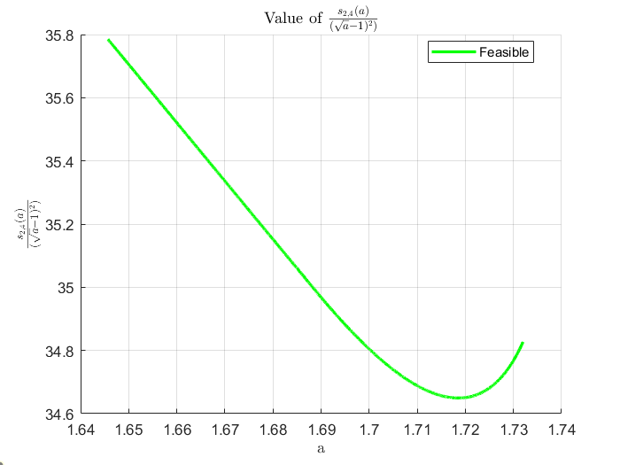
For each subproblem $Q_{2,i}(a)$ , a graph (see Figure 6 and Figure 7) is generated plotting the ratio $\displaystyle{}\frac{p_{2,i}(a)}{(\sqrt{a}-1)^{2}}$ against $a$ . In these graphs, we use different colors to represent the feasible and infeasible solutions to the original problem $Q_{2}(a)$ . The red points are used to indicate infeasible solutions that are the solutions of subproblems but do not satisfy all the constraints of problem $Q_{2}(a)$ . On the other hand, the green points represent feasible solutions that satisfy all constraints.

Then, the value of $q_{2}(a)$ could be obtained by comparing the optimal values of the subproblems $q_{2,1}(a)$ and $q_{2,2}(a)$ (only consider the value feasible to the problem $Q_{2}(a)$ ). The Figure 8 shows the ratio $\displaystyle{}\frac{q_{2}(a)}{(\sqrt{a}-1)^{2}}$ .

Then, the infimum of the ratio is determined to be $34.8992259$ , which could be achieved at several points, such as

q=[0.2114174,0.5028451,0.6363167,0.5028452,0.2114174,0].

The polynomial corresponding to this solution is,

f(\phi)=a_{0}+a_{1}\cos\phi+a_{2}\cos 2\phi+a_{3}\cos 3\phi+a_{4}\cos 4\phi+a_{5}\cos 5\phi,

where

	$\displaystyle a_{0}$	$\displaystyle=1,$
	$\displaystyle a_{1}$	$\displaystyle=1.7051159,$
	$\displaystyle a_{2}$	$\displaystyle=1.0438202,$
	$\displaystyle a_{3}$	$\displaystyle=0.4252409,$
	$\displaystyle a_{4}$	$\displaystyle=0.0893946,$
	$\displaystyle a_{5}$	$\displaystyle=0.$

One could see that this point $q$ also lies in the feasible region of $Q_{1}(a_{1})$ . This implies that the optimal solution of problem $Q_{2}(a_{1})$ is also the optimal solution of problem $Q_{1}(a_{1})$ and thus agrees with the value of $\chi_{5}(a_{1})$ . By the relationship

\frac{\chi_{5}(a)}{(\sqrt{a}-1)^{2}}\geq\frac{q_{2}(a)}{(\sqrt{a}-1)^{2}},

one can conclude

	$\displaystyle V_{5}$	$\displaystyle=\inf_{a\in\displaystyle{}\left[1.5597515,2\cos\frac{\pi}{7}\right]}\frac{\chi_{5}(a)}{(\sqrt{a}-1)^{2}}$
		$\displaystyle=\inf_{a\in\displaystyle{}\left[1.5597515,2\cos\frac{\pi}{7}\right]}\frac{q_{2}(a)}{(\sqrt{a}-1)^{2}}$
		$\displaystyle=34.8992259.$

This completes the proof.

∎

6 Exact value of $V_{6}$ .

In this section, we will determine the exact value of $V_{6}$ . From Equation (1.2), we have

V_{6}=\inf_{a\in\left(1,2\displaystyle{}\cos\frac{\pi}{8}\right]}\frac{\chi_{6}(a)}{(\sqrt{a}-1)^{2}},

where $\chi_{6}(a)$ is defined as

\chi_{6}(a)=\inf\left\{f(0)-1\mid f(\phi)\in C_{6},a_{0}\left(f\right)=1\text{ and }a_{1}\left(f\right)=a\right\}.

6.1 Exact value of $V_{6}$ .

In order to find the exact value of $V_{6}$ , we will use the Karush-Kuhn-Tucker conditions and the penalty function method to solve the optimization problem $\chi_{6}(a)$ . However, before proceeding, we first restrict the range of a to a smaller interval.

By a similar proof in Theorem 5.1, we have the following theorem.

Theorem 6.1.

The exact value of $V_{6}$ could be obtained by

\displaystyle{}V_{6}=\inf_{a\in[1.6456659,1.8231801]}\frac{\chi_{6}(a)}{(\sqrt{a}-1)^{2}}.

Proof.

Since the set of cosine polynomials $C_{5}\subset C_{6}$ , one have $V_{6}\leq V_{5}=$ 34.8992259. However, by Theorem 4.1 and Theorem 4.2 , we have

	$\displaystyle V_{6}(a)\geq F_{1}(a)=\frac{2a-1}{(\sqrt{a}-1)^{2}}$
	$\displaystyle V_{6}(a)\geq F_{2}(a)=\frac{5.87267810a-6.87267810}{(\sqrt{a}-1)^{2}}$
	$\displaystyle V_{6}(a)\geq F_{3}(a)=\frac{16.5a-25.8011608}{(\sqrt{a}-1)^{2}}$

for $\displaystyle{}a\in\left(1,2\cos\frac{\pi}{8}\right]$ . Given function $F:(1,\infty)\rightarrow\mathbb{R}$ with the form

F(a)=\frac{Aa-B}{(\sqrt{a}-1)^{2}}

where $A,B$ are constant. Taking the derivative, one have

F^{\prime}(a)=\frac{B-A\sqrt{x}}{(\sqrt{x}-1)^{3}\sqrt{x}}

This implies when $A>B$ the function $F(a)$ is decreasing on the interval $(1,\infty)$ . On the other hand, when $A<B$ , the function increasing on the interval $\left(1,(B/A)^{2}\right]$ and decreasing on the interval $\left[(B/A)^{2},\infty\right)$ . Apply this on the function $F_{1}(a),F_{2}(a)$ and $F_{3}(a)$ , we found out $F_{1}(a)$ is a decreasing function on the interval $\displaystyle{}\left(1,2\cos\frac{\pi}{8}\right]$ . However, the function $F_{2}(a)$ is increasing on $(1,1.3695543]$ and is decreasing on the interval $\displaystyle{}\left[1.3695543,2\cos\frac{\pi}{8}\right]$ . At the same time, the function $F_{3}(a)$ is increasing on the interval $\displaystyle{}\left(1,2\cos\frac{\pi}{8}\right]$ . Now, given any $f(\phi)\in C_{6}$ with $a_{0}(f)=1,a_{1}(f)=a\in(1,1.5510971]$ , one has

v(f)\geq\frac{\chi(a)}{(\sqrt{a}-1)^{2}}\geq F_{1}(a)\geq F_{1}(1.5510971)=34.8992605>V_{5}.

Similarly, for any $f(\phi)\in C_{5}$ with $a_{0}(f)=1,a_{1}(f)=a\in[1.5510971,1.6456659]$ , one could obtain

v(f)\geq\frac{\chi(a)}{(\sqrt{a}-1)^{2}}\geq F_{2}(a)\geq F_{2}(1.6456659)=34.8992261>V_{5}

Finally, for any $\displaystyle{}f(\phi)\in C_{6}$ with $\displaystyle{}a_{0}(f)=1,a_{1}(f)=a\in\left[1.8231801,2\cos\frac{\pi}{8}\right]$ , one could obtain

v(f)\geq\frac{\chi(a)}{(\sqrt{a}-1)^{2}}\geq F_{3}(a)\geq F_{3}(1.8231801)=34.8992630>V_{6}

This completes the proof.

∎

By Fejer-Reisz theorem theorem, the problem of finding the $\chi_{6}(a)$ for $\displaystyle{}a\in\left(1,2\displaystyle{}\cos\frac{\pi}{8}\right]$ can be formalized as the minimization problem in $\mathbb{R}^{7}$ as:

Problem 6.1.

Consider the optimization problem $R_{1}(a)$ defined as follows:

	$R_{1}(a)$ : Minimize	$\displaystyle F(\mathbf{x})=(x_{0}+x_{1}+\ldots+x_{6})^{2}-1$
	subject to	$\displaystyle H_{1}(\mathbf{x})=x_{0}^{2}+x_{1}^{2}+x_{2}^{2}+\ldots+x_{6}^{2}=1,$
		$\displaystyle H_{2}(\mathbf{x})=2(x_{0}x_{1}+x_{1}x_{2}+\ldots+x_{5}x_{6})=a,$
		$\displaystyle G_{1}(\mathbf{x})=2(x_{0}x_{2}+x_{1}x_{3}+\ldots+x_{4}x_{6})\geq 0,$
		$\displaystyle G_{2}(\mathbf{x})=2(x_{0}x_{3}+x_{1}x_{4}+\ldots+x_{3}x_{6})\geq 0,$
		$\displaystyle\quad\quad\quad\vdots$
		$\displaystyle G_{5}(\mathbf{x})=2x_{0}x_{6}\geq 0.$

Define $r_{1}(a)$ as the optimal value of the objective function $F(\mathbf{x})$ for a given $a$ :

r_{1}(a)=\min_{\mathbf{x}}F(\mathbf{x})\quad\text{subject to the constraints of }R_{1}(a).

However, instead of consider Problem $R_{1}(a)$ with seven constraints, we will consider following problem with four constraints.

Problem 6.2.

Consider the optimization problem $R_{2}(a)$ defined as follows:

	Minimize	$\displaystyle F(\mathbf{x})=(x_{0}+x_{1}+\ldots+x_{6})^{2}-1$
	subject to	$\displaystyle H_{1}(\mathbf{x})=\sum_{i=0}^{6}x_{i}^{2}=1,$
		$\displaystyle H_{2}(\mathbf{x})=2\left(x_{0}x_{1}+x_{1}x_{2}+\ldots+x_{5}x_{6}\right)=a,$
		$\displaystyle G_{4}(\mathbf{x})=2\left(x_{0}x_{5}+x_{1}x_{6}\right)\geq 0,$
		$\displaystyle G_{5}(\mathbf{x})=2x_{0}x_{6}\geq 0.$

Define $r_{2}(a)$ as the optimal value of the objective function $F(\mathbf{x})$ for a given $a$ :

r_{2}(a)=\min_{\mathbf{x}}F(\mathbf{x})\quad\text{subject to the constraints of }R_{2}(a).

Since the feasible region of problem $R_{1}(a)$ is the subset of the feasible region of problem $R_{2}(a)$ , this implies

\chi_{6}(a)=r_{1}(a)\geq r_{2}(a).

If the optimal point of problem $R_{2}(a)$ also satisfies the condition $G_{1}(\mathbf{x}),G_{2}(\mathbf{x})\text{ and }G_{3}(\mathbf{x})$ , then the optimal point will lie inside the feasible region of problem $R_{1}(a)$ . In this case,

\chi_{6}(a)=r_{1}(a)=r_{2}(a).

Theorem 6.2.

The exact value of $V_{6}$ can be expressed as:

\displaystyle{}V_{6}=\inf_{a\in[1.6456659,1.8231801]}\frac{r_{2}(a)}{(\sqrt{a}-1)^{2}}=34.8992259.

The exact solution corresponding to this infimum could be obtained at the point

r=[0.2114174,0.5028451,0.6363167,0.5028452,0.2114174,0,0].

The polynomial corresponding to this solution is,

f(\phi)=a_{0}+a_{1}\cos\phi+a_{2}\cos 2\phi+a_{3}\cos 3\phi+a_{4}\cos 4\phi+a_{5}\cos 5\phi+a_{6}\cos 6\phi,

where

	$\displaystyle a_{0}$	$\displaystyle=1,$
	$\displaystyle a_{1}$	$\displaystyle=1.7051159,$
	$\displaystyle a_{2}$	$\displaystyle=1.0438202,$
	$\displaystyle a_{3}$	$\displaystyle=0.4252409,$
	$\displaystyle a_{4}$	$\displaystyle=0.0893946,$
	$\displaystyle a_{5}$	$\displaystyle=0,$
	$\displaystyle a_{6}$	$\displaystyle=0.$

Proof.

Fix an $a\in[1.64566600,1.82318005]$ ,we would first like to establish the numerical solution of the optimization problem $R_{2}(a)$ . By applying the Karush-Kuhn-Tucker conditions (Theorem 3.3), if a point $\overline{\mathbf{x}}\in\mathbb{R}^{7}$ solves Problem $R_{2}(a)$ globally, there exist scalars $\lambda_{1},\lambda_{2},u_{1},$ and $u_{2}$ such that

$\displaystyle\nabla F(\overline{\mathbf{x}})+\sum_{i=1}^{2}\lambda_{i}\nabla H_{i}(\overline{\mathbf{x}})+\sum_{i=1}^{2}u_{i}\nabla G_{3+i}(\overline{\mathbf{x}})$	$\displaystyle=\mathbf{0}$		(6.1)
$\displaystyle u_{i}G_{3+i}(\overline{\mathbf{x}})$	$\displaystyle=0$	$\displaystyle\text{ for }i=1,2$	(6.2)
$\displaystyle u_{i}$	$\displaystyle\geq 0$	$\displaystyle\text{ for }i=1,2$	(6.3)

By the Equation (6.2), the problem $R_{2}(a)$ could be divided into following four subproblems, we call them problem $R_{2,1}(a),R_{2,2}(a),R_{2,3}(a)$ and $R_{2,4}(a)$ respectively. We will use $r_{2,1}(a),r_{2,2}(a),r_{2,3}(a)$ and $r_{2,4}(a)$ to denote the solutions of these subproblems respecively. The first subcase is when $u_{1}=0,u_{2}=0$ , the minimization problem corresponding to this subcase is

	$R_{2,1}(a)$ : Minimize	$\displaystyle F(\mathbf{x})=(x_{0}+x_{1}+\ldots+x_{6})^{2}-1$
	subject to	$\displaystyle H_{1}(\mathbf{x})=x_{0}^{2}+x_{1}^{2}+x_{2}^{2}+\ldots+x_{6}^{2}=1,$
		$\displaystyle H_{2}(\mathbf{x})=2(x_{0}x_{1}+x_{1}x_{2}+\ldots+x_{5}x_{6})=a.$

The second subcase is when $u_{1}\neq 0,u_{2}=0$ , the minimization problem corresponding to this subcase is

	$R_{2,2}(a)$ : Minimize	$\displaystyle F(\mathbf{x})=(x_{0}+x_{1}+\ldots+x_{6})^{2}-1$
	subject to	$\displaystyle H_{1}(\mathbf{x})=x_{0}^{2}+x_{1}^{2}+x_{2}^{2}+\ldots+x_{6}^{2}=1,$
		$\displaystyle H_{2}(\mathbf{x})=2(x_{0}x_{1}+x_{1}x_{2}+\ldots+x_{5}x_{6})=a,$
		$\displaystyle G_{4}(\mathbf{x})=2(x_{0}x_{5}+x_{1}x_{6})=0.$

The third subcase is when $u_{1}=0,u_{2}\neq 0$ , the minimization problem corresponding to this subcase is

	$R_{2,3}(a)$ : Minimize	$\displaystyle F(\mathbf{x})=(x_{0}+x_{1}+\ldots+x_{6})^{2}-1$
	subject to	$\displaystyle H_{1}(\mathbf{x})=x_{0}^{2}+x_{1}^{2}+x_{2}^{2}+\ldots+x_{6}^{2}=1,$
		$\displaystyle H_{2}(\mathbf{x})=2(x_{0}x_{1}+x_{1}x_{2}+\ldots+x_{5}x_{6})=a,$
		$\displaystyle G_{5}(\mathbf{x})=2x_{0}x_{6}=0.$

The fourth subcase is when $u_{1}\neq 0,u_{2}\neq 0$ , the minimization problem corresponding to this subcase is

	$R_{2,4}(a)$ : Minimize	$\displaystyle F(\mathbf{x})=(x_{0}+x_{1}+\ldots+x_{6})^{2}-1$
	subject to	$\displaystyle H_{1}(\mathbf{x})=x_{0}^{2}+x_{1}^{2}+x_{2}^{2}+\ldots+x_{6}^{2}=1,$
		$\displaystyle H_{2}(\mathbf{x})=2(x_{0}x_{1}+x_{1}x_{2}+\ldots+x_{5}x_{6})=a,$
		$\displaystyle G_{4}(\mathbf{x})=2(x_{0}x_{5}+x_{1}x_{6})=0,$
		$\displaystyle G_{5}(\mathbf{x})=2x_{0}x_{6}=0.$

By penalty function method (Theorem 3.4), for $i=1,2,3,4$ , we have

r_{2,i}(a)=\lim_{\mu\to\infty}\theta_{i}(\mu),

where

	$\displaystyle\theta_{1}(\mu)$	$\displaystyle=\inf\left\{F(\mathbf{x})+\mu\left((H_{1}(\mathbf{x})-1)^{2}+(H_{2}(\mathbf{x})-a)^{2}\right)\mid\mathbf{x}\in\mathbb{R}^{7}\right\},$
	$\displaystyle\theta_{2}(\mu)$	$\displaystyle=\inf\left\{F(\mathbf{x})+\mu\left((H_{1}(\mathbf{x})-1)^{2}+(H_{2}(\mathbf{x})-a)^{2}+G_{4}(\mathbf{x})^{2}\right)\mid\mathbf{x}\in\mathbb{R}^{7}\right\},$
	$\displaystyle\theta_{3}(\mu)$	$\displaystyle=\inf\left\{F(\mathbf{x})+\mu\left((H_{1}(\mathbf{x})-1)^{2}+(H_{2}(\mathbf{x})-a)^{2}+G_{5}(\mathbf{x})^{2}\right)\mid\mathbf{x}\in\mathbb{R}^{7}\right\},$
	$\displaystyle\theta_{4}(\mu)$	$\displaystyle=\inf\left\{F(\mathbf{x})+\mu\left((H_{1}(\mathbf{x})-1)^{2}+(H_{2}(\mathbf{x})-a)^{2}+\sum_{i=1}^{2}G_{3+i}(\mathbf{x})^{2}\right)\mid\mathbf{x}\in\mathbb{R}^{7}\right\}.$

Then, a Matlab-based algorithm is employed to compute the $\displaystyle{}\frac{r_{2,i}(a)}{(\sqrt{a}-1)^{2}}$ for $i=1,2,3,4$ . The algorithm employs the Newton-Raphson method, combined with a penalty function approach to iteratively minimize the penalized objective function (see Appendix B for the full Matlab implementation).

For each subproblem $R_{2,i}(a)$ , a graph (see Figure9, Figure10, Figure11 and Figure12) is generated plotting the ratio $\displaystyle{}\frac{r_{2,i}(a)}{(\sqrt{a}-1)^{2}}$ against $a$ . In these graphs, different colors are used to distinguish between feasible and infeasible solutions to the original problem $R_{2}(a)$ . Red points indicate infeasible solutions, which solve subproblems but fail to meet all the constraints, while green points represent feasible solutions that satisfy all constraints.

Among all feasible solutions for each $a$ , $r_{2}(a)$ is identified as the minimum value of all $r_{2,i}(a)$ that are feasible to the problem $R_{2}(a)$ . Figure 13 shows the graph plotting the ratio of the function $\frac{r_{2}(a)}{(\sqrt{a}-1)^{2}}$ .

Then, the infimum of the ratio is determined to be $34.899226$ , achieved at a specific point in $\mathbb{R}^{7}$ . This point is given by

r=[0.2114174,0.5028451,0.6363167,0.5028452,0.2114174,0,0].

The polynomial corresponding to this point is,

f(\phi)=a_{0}+a_{1}\cos\phi+a_{2}\cos 2\phi+a_{3}\cos 3\phi+a_{4}\cos 4\phi+a_{5}\cos 5\phi+a_{6}\cos 6\phi,

where

	$\displaystyle a_{0}$	$\displaystyle=1,$
	$\displaystyle a_{1}$	$\displaystyle=1.7051159,$
	$\displaystyle a_{2}$	$\displaystyle=1.0438202,$
	$\displaystyle a_{3}$	$\displaystyle=0.4252409,$
	$\displaystyle a_{4}$	$\displaystyle=0.0893946,$
	$\displaystyle a_{5}$	$\displaystyle=0,$
	$\displaystyle a_{6}$	$\displaystyle=0.$

One could see that this point $r$ also lies in the feasible region of $R_{1}(a_{1})$ . This implies that the optimal solution of problem $R_{2}(a_{1})$ is also the optimal solution of problem $R_{1}(a_{1})$ and thus agrees with the value of $\chi_{6}(a_{1})$ . By the relationship

\frac{\chi_{6}(a)}{(\sqrt{a}-1)^{2}}\geq\frac{r_{2}(a)}{(\sqrt{a}-1)^{2}},

one can conclude

	$\displaystyle V_{6}$	$\displaystyle=\inf_{a\in\displaystyle{}[1.6456659,1.8231801]}\frac{\chi_{6}(a)}{(\sqrt{a}-1)^{2}}$
		$\displaystyle=\inf_{a\in\displaystyle{}[1.6456659,1.8231801]}\frac{r_{2}(a)}{(\sqrt{a}-1)^{2}}$
		$\displaystyle=34.8992259.$

This completes the proof.

∎

7 Exact value of $V_{7}$ .

This section will be devoted to find the exact value of $V_{7}$ . First of all, by Equation (1.2), we have

\displaystyle{}V_{7}=\inf_{a\in\left(1,2\displaystyle{}\cos\frac{\pi}{9}\right]}\frac{\chi_{7}(a)}{(\sqrt{a}-1)^{2}},

where

\chi_{7}(a)=\inf\left\{f(0)-1\mid f(\phi)\in C_{7},a_{0}\left(f\right)=1\text{ and }a_{1}\left(f\right)=a\right\}\text{. }

7.1 Exact value of $V_{7}$ .

In order to find the exact value of $V_{7}$ , we will use the Karush-Kuhn-Tucker conditions and the penalty function method to solve the optimization problem $\chi_{7}(a)$ . Before proceeding, we first restrict the range of a to a smaller interval.

By the same proof in Theorem 6.1, we have the following theorem.

Theorem 7.1.

The exact value of $V_{7}$ could be obtained by

\displaystyle{}V_{7}=\inf_{a\in a\in[1.6456659,1.8231801]}\frac{\chi_{7}(a)}{(\sqrt{a}-1)^{2}}.

By Fejer-Reisz theorem theorem, the problem of finding the $\chi_{7}(a)$ for $\displaystyle{}a\in\left(1,2\displaystyle{}\cos\frac{\pi}{9}\right]$ can be formalised as the following minimization problem in $\mathbb{R}^{8}$ .

Problem 7.1.

Consider the optimization problem $S_{1}(a)$ defined as follows:

	$S_{1}(a)$ : Minimize	$\displaystyle F(\mathbf{x})=(x_{0}+x_{1}+\ldots+x_{7})^{2}-1$
	subject to	$\displaystyle H_{1}(\mathbf{x})=x_{0}^{2}+x_{1}^{2}+x_{2}^{2}+\ldots+x_{7}^{2}=1,$
		$\displaystyle H_{2}(\mathbf{x})=2(x_{0}x_{1}+x_{1}x_{2}+\ldots+x_{6}x_{7})=a,$
		$\displaystyle G_{1}(\mathbf{x})=2(x_{0}x_{2}+x_{1}x_{3}+\ldots+x_{5}x_{7})\geq 0,$
		$\displaystyle G_{2}(\mathbf{x})=2(x_{0}x_{3}+x_{1}x_{4}+\ldots+x_{4}x_{7})\geq 0,$
		$\displaystyle\quad\quad\quad\vdots$
		$\displaystyle G_{6}(\mathbf{x})=2x_{0}x_{7}\geq 0.$

Define $s_{1}(a)$ as the optimal value of the objective function $F(\mathbf{x})$ for a given $a$ :

s_{1}(a)=\min_{\mathbf{x}}F(\mathbf{x})\quad\text{subject to the constraints of }S_{1}(a).

However, instead of consider Problem $S_{1}(a)$ with eight constraints, we will consider following problem with four constraints.

Problem 7.2.

Consider the optimization problem $S_{2}(a)$ defined as follows:

	$S_{2}(a)$ : Minimize	$\displaystyle F(\mathbf{x})=(x_{0}+x_{1}+\ldots+x_{7})^{2}-1$
	subject to	$\displaystyle H_{1}(\mathbf{x})=x_{0}^{2}+x_{1}^{2}+x_{2}^{2}+\ldots+x_{7}^{2}=1,$
		$\displaystyle H_{2}(\mathbf{x})=2(x_{0}x_{1}+x_{1}x_{2}+\ldots+x_{6}x_{7})=a,$
		$\displaystyle G_{4}(\mathbf{x})=2(x_{0}x_{5}+x_{1}x_{6}+x_{2}x_{7})\geq 0,$
		$\displaystyle G_{5}(\mathbf{x})=2(x_{0}x_{6}+x_{1}x_{7})\geq 0.$

Define $s_{2}(a)$ as the optimal value of the objective function $F(\mathbf{x})$ for a given $a$ :

s_{2}(a)=\min_{\mathbf{x}}F(\mathbf{x})\quad\text{subject to the constraints of }S_{2}(a).

Since the feasible region of problem $S_{1}(a)$ is the subset of the feasible region of problem $S_{2}(a)$ , this implies

\chi_{7}(a)=s_{1}(a)\geq s_{2}(a).

If the optimal point of problem $S_{2}(a)$ also satisfies the condition $G_{1}(\mathbf{x}),G_{2}(\mathbf{x}),G_{3}(\mathbf{x}),\text{ and }G_{6}(\mathbf{x})$ , then the optimal point will lie inside the feasible region of problem $S_{1}(a)$ . In this case,

\chi_{7}(a)=s_{1}(a)=s_{2}(a).

Theorem 7.2.

The exact value of $V_{7}$ can be expressed as:

\displaystyle{}V_{7}=\inf_{a\in a\in[1.6456659,1.8231801]}\frac{\chi_{7}(a)}{(\sqrt{a}-1)^{2}}=34.6494874.

The exact solution corresponding to this infimum could be obtained at the point

	$\displaystyle s$	$\displaystyle=[0.1685903,0.4506317,0.6267577,0.5454191,$
		$\displaystyle 0.2756348,0.0361770,-0.0282171,0.1055656].$

The polynomial corresponding to this solution is,

	$\displaystyle f(\phi)=$	$\displaystyle a_{0}+a_{1}\cos\phi+a_{2}\cos 2\phi+a_{3}\cos 3\phi+a_{4}\cos 4\phi$
		$\displaystyle+a_{5}\cos 5\phi+a_{6}\cos 6\phi+a_{7}\cos 7\phi,$

where

	$\displaystyle a_{0}$	$\displaystyle=1,$
	$\displaystyle a_{1}$	$\displaystyle=1.7185098,$
	$\displaystyle a_{2}$	$\displaystyle=1.0731034,$
	$\displaystyle a_{3}$	$\displaystyle=0.4527292,$
	$\displaystyle a_{4}$	$\displaystyle=0.1016950,$
	$\displaystyle a_{5}$	$\displaystyle=0,$
	$\displaystyle a_{6}$	$\displaystyle=0,$
	$\displaystyle a_{7}$	$\displaystyle=0.0035595.$

Proof.

Fix an $a\in[1.6456659,1.8231801]$ , we would first like to establish the numerical solution of the optimization problem $S_{2}(a)$ . By applying the Karush-Kuhn-Tucker conditions (Theorem 3.3), if a point $\overline{\mathbf{x}}\in\mathbb{R}^{8}$ solves Problem $S_{2}(a)$ globally, there exist scalars $\lambda_{1},\lambda_{2},u_{1},$ and $u_{2}$ such that

$\displaystyle\nabla F(\overline{\mathbf{x}})+\sum_{i=1}^{2}\lambda_{i}\nabla H_{i}(\overline{\mathbf{x}})+\sum_{i=1}^{2}u_{i}\nabla G_{3+i}(\overline{\mathbf{x}})$	$\displaystyle=\mathbf{0}$		(7.1)
$\displaystyle u_{i}G_{3+i}(\overline{\mathbf{x}})$	$\displaystyle=0$	$\displaystyle\text{ for }i=1,2$	(7.2)
$\displaystyle u_{i}$	$\displaystyle\geq 0$	$\displaystyle\text{ for }i=1,2$	(7.3)

By the Equation (7.2), the problem $S_{2}(a)$ could be divided into the following four subproblems, we call them problem $S_{2,1}(a),S_{2,2}(a),S_{2,3}(a)$ and $S_{2,4}(a)$ respectively. We will use $s_{2,1}(a),s_{2,2}(a),s_{2,3}(a)$ and $s_{2,4}(a)$ to denote the solutions of these subproblems respectively. The first subcase is when $u_{1}=0,u_{2}=0$ , the minimization problem corresponding to this subcase is

	$S_{2,1}(a)$ : Minimize	$\displaystyle F(\mathbf{x})=(x_{0}+x_{1}+\ldots+x_{7})^{2}-1$
	subject to	$\displaystyle H_{1}(\mathbf{x})=x_{0}^{2}+x_{1}^{2}+x_{2}^{2}+\ldots+x_{7}^{2}=1,$
		$\displaystyle H_{2}(\mathbf{x})=2(x_{0}x_{1}+x_{1}x_{2}+\ldots+x_{6}x_{7})=a.$

The second subcase is when $u_{1}\neq 0,u_{2}=0$ , the minimization problem corresponding to this subcase is

	$S_{2,2}(a)$ : Minimize	$\displaystyle F(\mathbf{x})=(x_{0}+x_{1}+\ldots+x_{7})^{2}-1$
	subject to	$\displaystyle H_{1}(\mathbf{x})=x_{0}^{2}+x_{1}^{2}+x_{2}^{2}+\ldots+x_{7}^{2}=1,$
		$\displaystyle H_{2}(\mathbf{x})=2(x_{0}x_{1}+x_{1}x_{2}+\ldots+x_{6}x_{7})=a,$
		$\displaystyle G_{4}(\mathbf{x})=2(x_{0}x_{5}+x_{1}x_{6}+x_{2}x_{7})=0.$

The third subcase is when $u_{1}=0,u_{2}\neq 0$ , the minimization problem corresponding to this subcase is

	$S_{2,3}(a)$ : Minimize	$\displaystyle F(\mathbf{x})=(x_{0}+x_{1}+\ldots+x_{7})^{2}-1$
	subject to	$\displaystyle H_{1}(\mathbf{x})=x_{0}^{2}+x_{1}^{2}+x_{2}^{2}+\ldots+x_{7}^{2}=1,$
		$\displaystyle H_{2}(\mathbf{x})=2(x_{0}x_{1}+x_{1}x_{2}+\ldots+x_{6}x_{7})=a,$
		$\displaystyle G_{5}(\mathbf{x})=2(x_{0}x_{6}+x_{1}x_{7})=0.$

The fourth subcase is when $u_{1}\neq 0,u_{2}\neq 0$ , the minimization problem corresponding to this subcase is

	$S_{2,4}(a)$ : Minimize	$\displaystyle F(\mathbf{x})=(x_{0}+x_{1}+\ldots+x_{7})^{2}-1$
	subject to	$\displaystyle H_{1}(\mathbf{x})=x_{0}^{2}+x_{1}^{2}+x_{2}^{2}+\ldots+x_{7}^{2}=1,$
		$\displaystyle H_{2}(\mathbf{x})=2(x_{0}x_{1}+x_{1}x_{2}+\ldots+x_{6}x_{7})=a,$
		$\displaystyle G_{4}(\mathbf{x})=2(x_{0}x_{5}+x_{1}x_{6}+x_{2}x_{7})=0,$
		$\displaystyle G_{5}(\mathbf{x})=2(x_{0}x_{6}+x_{1}x_{7})=0.$

By penalty function method (Theorem 3.4), for $i=1,2,3,4$ , we have

s_{2,i}(a)=\lim_{\mu\to\infty}\theta_{i}(\mu),

where

	$\displaystyle\theta_{1}(\mu)$	$\displaystyle=\inf\left\{F(\mathbf{x})+\mu\left((H_{1}(\mathbf{x})-1)^{2}+(H_{2}(\mathbf{x})-a)^{2}\right)\mid\mathbf{x}\in\mathbb{R}^{8}\right\},$
	$\displaystyle\theta_{2}(\mu)$	$\displaystyle=\inf\left\{F(\mathbf{x})+\mu\left((H_{1}(\mathbf{x})-1)^{2}+(H_{2}(\mathbf{x})-a)^{2}+G_{4}(\mathbf{x})^{2}\right)\mid\mathbf{x}\in\mathbb{R}^{8}\right\},$
	$\displaystyle\theta_{3}(\mu)$	$\displaystyle=\inf\left\{F(\mathbf{x})+\mu\left((H_{1}(\mathbf{x})-1)^{2}+(H_{2}(\mathbf{x})-a)^{2}+G_{5}(\mathbf{x})^{2}\right)\mid\mathbf{x}\in\mathbb{R}^{8}\right\},$
	$\displaystyle\theta_{4}(\mu)$	$\displaystyle=\inf\left\{F(\mathbf{x})+\mu\left((H_{1}(\mathbf{x})-1)^{2}+(H_{2}(\mathbf{x})-a)^{2}+\sum_{i=1}^{2}G_{3+i}(\mathbf{x})^{2}\right)\mid\mathbf{x}\in\mathbb{R}^{8}\right\}.$

A Matlab-based algorithm is subsequently used to calculate $\displaystyle{}\frac{s_{2,i}(a)}{(\sqrt{a}-1)^{2}}$ for $i=1,2,3,4$ , by adopting the Newton-Raphson method in conjunction with a penalty function technique to iteratively find the minimizer of the penalized objective function (see Appendix B for the detailed Matlab implementation).

For each subproblem $S_{2,i}(a)$ , a graph (Figure14, Figure15, Figure16 and Figure17) is generated plotting the ratio $\displaystyle{}\frac{s_{2,i}(a)}{(\sqrt{a}-1)^{2}}$ against $a$ . In these graphs, different colors are used to show feasible and infeasible solutions to the original problem $S_{2}(a)$ . Red points indicate infeasible solutions that solve the subproblems but do not meet all constraints of $S_{2}(a)$ . On the other hand, green points represent feasible solutions that satisfy all the constraints.

Among all feasible solutions for each $a$ , $s_{2}(a)$ is identified as the minimum value of all $s_{2,i}(a)$ that are feasible to the problem $S_{2}(a)$ . Figure 18 shows the graph plotting the ratio of the function $\displaystyle{}\frac{s_{2}(a)}{(\sqrt{a}-1)^{2}}$ .

Then, the infimum of the ratio is determined to be $34.64948641$ , achieved at a specific point in $\mathbb{R}^{8}$ . This point is given by

	$\displaystyle s$	$\displaystyle=[0.1685903,0.4506317,0.6267577,0.5454191,$
		$\displaystyle 0.2756348,0.0361770,-0.0282171,0.1055656].$

The polynomial corresponding to this solution is,

f(\phi)=a_{0}+a_{1}\cos\phi+a_{2}\cos 2\phi+a_{3}\cos 3\phi+a_{4}\cos 4\phi+a_{5}\cos 5\phi+a_{6}\cos 6\phi,

where

	$\displaystyle a_{0}$	$\displaystyle=1,$
	$\displaystyle a_{1}$	$\displaystyle=1.7185098,$
	$\displaystyle a_{2}$	$\displaystyle=1.0731034,$
	$\displaystyle a_{3}$	$\displaystyle=0.4527292,$
	$\displaystyle a_{4}$	$\displaystyle=0.101695001,$
	$\displaystyle a_{5}$	$\displaystyle=0,$
	$\displaystyle a_{6}$	$\displaystyle=0,$
	$\displaystyle a_{7}$	$\displaystyle=0.003559468.$

One could see that this point $s$ also lies in the feasible region of $S_{1}\left(a_{1}\right)$ . This implies that the optimal solution of problem $S_{2}\left(a_{1}\right)$ is also the optimal solution of problem $S_{1}\left(a_{1}\right)$ and thus agrees with the value of $\chi_{7}\left(a_{1}\right)$ . By the relationship

\frac{\chi_{7}(a)}{(\sqrt{a}-1)^{2}}\geq\frac{s_{2}(a)}{(\sqrt{a}-1)^{2}},

one can conclude

	$\displaystyle V_{7}$	$\displaystyle=\inf_{a\in\displaystyle{}[1.6456659,1.8231801]}\frac{\chi_{7}(a)}{(\sqrt{a}-1)^{2}}$
		$\displaystyle=\inf_{a\in\displaystyle{}[1.6456659,1.8231801]}\frac{s_{2}(a)}{(\sqrt{a}-1)^{2}}$
		$\displaystyle=34.6494874.$

This completes the proof. ∎

8 Exact value of $V_{8}$ .

In this section, we aim to determine the exact value of $V_{8}$ , following the same approach as in the previous sections. From Equation (1.2), the value of $V_{8}$ is given by

V_{8}=\inf_{a\in\left(1,2\displaystyle{}\cos\frac{\pi}{10}\right]}\frac{\chi_{8}(a)}{(\sqrt{a}-1)^{2}},

where

\chi_{8}(a)=\inf\left\{f(0)-1\mid f(\phi)\in C_{8},a_{0}\left(f\right)=1\text{ and }a_{1}\left(f\right)=a\right\}\text{. }

8.1 Exact value of $V_{8}$ .

In order to find the exact value of $V_{8}$ , we will use the Karush-Kuhn-Tucker conditions and the penalty function method to solve the optimization problem $\chi_{8}(a)$ . To begin, we will narrow the range of a to a smaller interval.

By a similar proof in Theorem 6.1, we have the following theorem.

Theorem 8.1.

The exact value of $V_{8}$ could be obtained by

V_{8}=\inf_{a\in[1.6566924,1.8191095]}\frac{\chi_{8}(a)}{(\sqrt{a}-1)^{2}}.

Proof.

Since the set of cosine polynomials $C_{7}\subset C_{8}$ , one have $V_{8}\leq V_{7}=34.6494874$ . However, by Theorem 4.1 and Theorem 4.2, we have

$\displaystyle V_{8}(a)$	$\displaystyle\geq F_{1}(a)=\frac{2a-1}{(\sqrt{a}-1)^{2}},$	(8.1)
$\displaystyle V_{8}(a)$	$\displaystyle\geq F_{2}(a)=\frac{5.87267810a-6.87267810}{(\sqrt{a}-1)^{2}},$	(8.2)
$\displaystyle V_{8}(a)$	$\displaystyle\geq F_{3}(a)=\frac{16.5a-25.8011608}{(\sqrt{a}-1)^{2}}.$	(8.3)

for $a\in\left(1,2\displaystyle{}\cos\frac{\pi}{10}\right].$ Given function $F:(1,\infty)\to\mathbb{R}$ with the form

F(a)=\frac{Aa-B}{(\sqrt{a}-1)^{2}},

where $A,B$ are constant. Taking the derivative, one has

F^{\prime}(a)=\frac{B-A\sqrt{x}}{(\sqrt{x}-1)^{3}\sqrt{x}}.

This implies when $A>B$ the function $F(a)$ is decreasing on the interval $(1,\infty)$ . On the other hand, when $A<B$ , the function increasing on the interval $\displaystyle{}\left(1,(B/A)^{2}\right]$ and decreasing on the interval $\displaystyle{}[(B/A)^{2},\infty)$ . Apply this on the function $F_{1}(a),F_{2}(a)$ and $F_{3}(a)$ , we found out $F_{1}(a)$ is a decreasing function on the interval $\displaystyle{}\left(1,2\cos\frac{\pi}{10}\right]$ . However, the function $F_{2}(a)$ is increasing on $(1,1.3695543]$ and is decreasing on the interval $\displaystyle{}\left[1.36955543,2\cos\frac{\pi}{10}\right]$ . On the same time the function $F_{3}(a)$ is increasing on the interval $\displaystyle{}\left(1,2\cos\frac{\pi}{10}\right]$ .

Now, given any $f(\phi)\in C_{8}$ with $a_{0}(f)=1,a_{1}(f)=a\in(1,1.5542038]$ , one has

v(f)\geq\frac{\chi(a)}{(\sqrt{a}-1)^{2}}\geq F_{1}(a)\geq F_{1}(1.5542038)=34.6494937>V_{8}.

Similarly, for any $f(\phi)\in C_{8}$ with $a_{0}(f)=1,a_{1}(f)=a\in[1.5542038,1.6566924]$ , one could obtain

v(f)\geq\frac{\chi(a)}{(\sqrt{a}-1)^{2}}\geq F_{2}(a)\geq F_{2}(1.6566924)=34.6494895>V_{8}.

Finally, for any $f(\phi)\in C_{8}$ with $a_{0}(f)=1,a_{1}(f)=a\in\left[1.8191095,2\cos\frac{\pi}{10}\right]$ , one could obtain

v(f)\geq\frac{\chi(a)}{(\sqrt{a}-1)^{2}}\geq F_{3}(a)\geq F_{3}(1.8191095)=34.6494933>V_{8}.

This completes the proof. ∎

By Fejer-Reisz theorem, the problem of finding the $\chi_{8}(a)$ for $\displaystyle{}a\in\left(1,2\displaystyle{}\cos\frac{\pi}{10}\right]$ can be formalized as the minimization problem in $\mathbb{R}^{9}$ as:

Problem 8.1.

Consider the optimization problem $T_{1}(a)$ defined as follows:

	$T_{1}(a)$ : Minimize	$\displaystyle F(\mathbf{x})=(x_{0}+x_{1}+\ldots+x_{8})^{2}-1$
	subject to	$\displaystyle H_{1}(\mathbf{x})=x_{0}^{2}+x_{1}^{2}+x_{2}^{2}+\ldots+x_{8}^{2}=1,$
		$\displaystyle H_{2}(\mathbf{x})=2(x_{0}x_{1}+x_{1}x_{2}+\ldots+x_{7}x_{8})=a,$
		$\displaystyle G_{1}(\mathbf{x})=2(x_{0}x_{2}+x_{1}x_{3}+\ldots+x_{6}x_{8})\geq 0,$
		$\displaystyle G_{2}(\mathbf{x})=2(x_{0}x_{3}+x_{1}x_{4}+\ldots+x_{5}x_{8})\geq 0,$
		$\displaystyle\quad\quad\quad{\vdots}$
		$\displaystyle G_{7}(\mathbf{x})=2x_{0}x_{8}\geq 0.$

Define $t_{1}(a)$ as the optimal value of the objective function $F(\mathbf{x})$ for a given $a$ :

t_{1}(a)=\min_{\mathbf{x}}F(\mathbf{x})\quad\text{subject to the constraints of }T_{1}(a).

However, instead of considering Problem $T_{1}(a)$ with nine constraints, we will consider the following problem with four constraints.

Problem 8.2.

Consider the optimization problem $T_{2}(a)$ defined as follows:

	$T_{2}(a)$ : Minimize	$\displaystyle F(\mathbf{x})=(x_{0}+x_{1}+\ldots+x_{8})^{2}-1$
	subject to	$\displaystyle H_{1}(\mathbf{x})=x_{0}^{2}+x_{1}^{2}+x_{2}^{2}+\ldots+x_{8}^{2}=1,$
		$\displaystyle H_{2}(\mathbf{x})=2(x_{0}x_{1}+x_{1}x_{2}+\ldots+x_{7}x_{8})=a,$
		$\displaystyle G_{4}(\mathbf{x})=2(x_{0}x_{5}+x_{1}x_{6}+x_{2}x_{7}+x_{3}x_{8})\geq 0,$
		$\displaystyle G_{5}(\mathbf{x})=2(x_{0}x_{6}+x_{1}x_{7}+x_{2}x_{8})\geq 0.$

Define $t_{2}(a)$ as the optimal value of the objective function $F(\mathbf{x})$ for a given $a$ :

t_{2}(a)=\min_{\mathbf{x}}F(\mathbf{x})\quad\text{subject to the constraints of }T_{2}(a).

Since the feasible region of problem $T_{1}(a)$ is the subset of the feasible region of problem $T_{2}(a)$ , this implies

\chi_{8}(a)=t_{1}(a)\geq t_{2}(a).

If the optimal point of problem $T_{2}(a)$ also satisfies the condition $G_{1}(\mathbf{x}),G_{2}(\mathbf{x}),$ $G_{3}(\mathbf{x}),G_{6}(\mathbf{x}),$ and $G_{7}(\mathbf{x})$ , then the optimal point will lie inside the feasible region of problem $T_{1}(a)$ . This implies it will also be the solution of problem $T_{1}(a)$ . In this case,

\chi_{8}(a)=t_{1}(a)=t_{2}(a).

Theorem 8.2.

The exact value of $V_{8}$ can be expressed as:

V_{8}=\inf_{a\in[1.6566924,1.8191095]}\frac{t_{2}(a)}{(\sqrt{a}-1)^{2}}=34.5399155.

The exact solution corresponding to this infimum could be obtained at the point

	$\displaystyle t=$	$\displaystyle[0.1246536,0.3805581,0.5968565,0.5888198,0.3562317,$
		$\displaystyle 0.0912429,-0.0315349,-0.0146819,0.0159473]$

The polynomial corresponding to this solution is,

	$\displaystyle f(\phi)$	$\displaystyle=a_{0}+a_{1}\cos\phi+a_{2}\cos 2\phi+a_{3}\cos 3\phi+a_{4}\cos 4\phi$
		$\displaystyle+a_{5}\cos 5\phi+a_{6}\cos 6\phi+a_{7}\cos 7\phi+a_{8}\cos 8\phi,$

where

	$\displaystyle a_{0}$	$\displaystyle=1,$
	$\displaystyle a_{1}$	$\displaystyle=1.7312576,$
	$\displaystyle a_{2}$	$\displaystyle=1.1034980,$
	$\displaystyle a_{3}$	$\displaystyle=0.4821616,$
	$\displaystyle a_{4}$	$\displaystyle=0.1146858,$
	$\displaystyle a_{5}$	$\displaystyle=0,$
	$\displaystyle a_{6}$	$\displaystyle=0,$
	$\displaystyle a_{7}$	$\displaystyle=0.0084774,$
	$\displaystyle a_{8}$	$\displaystyle=0.0039758.$

Proof.

Fix an $a\in[1.6566924,1.8191095]$ , we would first like to establish the numerical solution of the optimization problem $T_{2}(a)$ . By applying the Karush-Kuhn-Tucker conditions (Theorem 3.3), if a point $\overline{\mathbf{x}}\in\mathbb{R}^{9}$ solves Problem $T_{2}(a)$ globally, there exist scalars $\lambda_{1},\lambda_{2},u_{1},u_{2}$ such that

$\displaystyle\nabla F(\overline{\mathbf{x}})+\sum_{i=1}^{2}\lambda_{i}\nabla H_{i}(\overline{\mathbf{x}})+\sum_{i=1}^{2}u_{i}\nabla G_{3+i}(\overline{\mathbf{x}})$	$\displaystyle=\mathbf{0}$		(8.4)
$\displaystyle u_{i}G_{3+i}(\overline{\mathbf{x}})$	$\displaystyle=0$	$\displaystyle\text{ for }i=1,2$	(8.5)
$\displaystyle u_{i}$	$\displaystyle\geq 0$	$\displaystyle\text{ for }i=1,2$	(8.6)

By the Equation (8.5), the problem $T_{2}(a)$ could be divided into the following four subproblems, we call them problem $T_{2,1}(a),T_{2,2}(a),T_{2,3}(a)$ and $T_{2,4}(a)$ respectively. We will use $t_{2,1}(a),t_{2,2}(a),t_{2,3}(a)$ and $t_{2,4}(a)$ to denote the solutions of these subproblems respectively. The first subcase is when $u_{1}=0,u_{2}=0$ , the minimization problem corresponding to this subcase is

	$T_{2,1}(a)$ : Minimize	$\displaystyle F(\mathbf{x})=(x_{0}+x_{1}+\ldots+x_{8})^{2}-1$
	subject to	$\displaystyle H_{1}(\mathbf{x})=x_{0}^{2}+x_{1}^{2}+x_{2}^{2}+\ldots+x_{8}^{2}=1,$
		$\displaystyle H_{2}(\mathbf{x})=2(x_{0}x_{1}+x_{1}x_{2}+\ldots+x_{7}x_{8})=a.$

The second subcase is when $u_{1}\neq 0,u_{2}=0$ , the minimization problem corresponding to this subcase is

	$T_{2,2}(a)$ : Minimize	$\displaystyle F(\mathbf{x})=(x_{0}+x_{1}+\ldots+x_{8})^{2}-1$
	subject to	$\displaystyle H_{1}(\mathbf{x})=x_{0}^{2}+x_{1}^{2}+x_{2}^{2}+\ldots+x_{8}^{2}=1,$
		$\displaystyle H_{2}(\mathbf{x})=2(x_{0}x_{1}+x_{1}x_{2}+\ldots+x_{7}x_{8})=a,$
		$\displaystyle G_{4}(\mathbf{x})=2(x_{0}x_{5}+x_{1}x_{6}+x_{2}x_{7}+x_{3}x_{8})=0.$

The third subcase is when $u_{1}=0,u_{2}\neq 0$ , the minimization problem corresponding to this subcase is

	$T_{2,3}(a)$ : Minimize	$\displaystyle F(\mathbf{x})=(x_{0}+x_{1}+\ldots+x_{8})^{2}-1$
	subject to	$\displaystyle H_{1}(\mathbf{x})=x_{0}^{2}+x_{1}^{2}+x_{2}^{2}+\ldots+x_{8}^{2}=1,$
		$\displaystyle H_{2}(\mathbf{x})=2(x_{0}x_{1}+x_{1}x_{2}+\ldots+x_{7}x_{8})=a,$
		$\displaystyle G_{5}(\mathbf{x})=2(x_{0}x_{6}+x_{1}x_{7}+x_{2}x_{8})=0.$

The fourth subcase is when $u_{1}\neq 0,u_{2}\neq 0$ , the minimization problem corresponding to this subcase is

	$T_{2,4}(a)$ : Minimize	$\displaystyle F(\mathbf{x})=(x_{0}+x_{1}+\ldots+x_{8})^{2}-1$
	subject to	$\displaystyle H_{1}(\mathbf{x})=x_{0}^{2}+x_{1}^{2}+x_{2}^{2}+\ldots+x_{8}^{2}=1,$
		$\displaystyle H_{2}(\mathbf{x})=2(x_{0}x_{1}+x_{1}x_{2}+\ldots+x_{7}x_{8})=a,$
		$\displaystyle G_{4}(\mathbf{x})=2(x_{0}x_{5}+x_{1}x_{6}+x_{2}x_{7}+x_{3}x_{8})=0,$
		$\displaystyle G_{5}(\mathbf{x})=2(x_{0}x_{6}+x_{1}x_{7}+x_{2}x_{8})=0.$

By penalty function method (Theorem 3.4), for $i=1,2,3,4$ , we have

t_{2,i}(a)=\lim_{\mu\to\infty}\theta_{i}(\mu),

where

	$\displaystyle\theta_{1}(\mu)$	$\displaystyle=\inf\left\{F(\mathbf{x})+\mu\left((H_{1}(\mathbf{x})-1)^{2}+(H_{2}(\mathbf{x})-a)^{2}\right)\mid\mathbf{x}\in\mathbb{R}^{9}\right\},$
	$\displaystyle\theta_{2}(\mu)$	$\displaystyle=\inf\left\{F(\mathbf{x})+\mu\left((H_{1}(\mathbf{x})-1)^{2}+(H_{2}(\mathbf{x})-a)^{2}+G_{4}(\mathbf{x})^{2}\right)\mid\mathbf{x}\in\mathbb{R}^{9}\right\},$
	$\displaystyle\theta_{3}(\mu)$	$\displaystyle=\inf\left\{F(\mathbf{x})+\mu\left((H_{1}(\mathbf{x})-1)^{2}+(H_{2}(\mathbf{x})-a)^{2}+G_{5}(\mathbf{x})^{2}\right)\mid\mathbf{x}\in\mathbb{R}^{9}\right\},$
	$\displaystyle\theta_{4}(\mu)$	$\displaystyle=\inf\left\{F(\mathbf{x})+\mu\left((H_{1}(\mathbf{x})-1)^{2}+(H_{2}(\mathbf{x})-a)^{2}+\sum_{i=1}^{2}G_{3+i}(\mathbf{x})^{2}\right)\mid\mathbf{x}\in\mathbb{R}^{9}\right\}.$

Then, a Matlab-based algorithm is employed to compute the $\displaystyle{}\frac{t_{2,i}(a)}{(\sqrt{a}-1)^{2}}$ for $i=1,2,3,4$ , through Newton-Raphson method and penalty function approach.

For each subproblem $t_{2,i}(a)$ , a graph (Figure 19, Figure 20, Figure 21 and Figure 22) is generated plotting the ratio $\displaystyle{}\frac{t_{2,i}(a)}{(\sqrt{a}-1)^{2}}$ against $a$ . Colors are utilized in the graphs to differentiate between feasible and infeasible solutions for the original problem $T_{2}(a)$ . Red points signify infeasible solutions that resolve subproblems but violate certain constraints, while green points represent feasible solutions that adhere to all constraints.

Among all feasible solutions for each $a$ , $t_{2}(a)$ is identified as the minimum value of all $t_{2,i}(a)$ that are feasible to the problem $T_{2}(a)$ . The following graph (Figure 23) is generated plotting the ratio of the function $\displaystyle{}\frac{t_{2}(a)}{(\sqrt{a}-1)^{2}}$ .

Then, the infimum of the ratio is determined to be $34.5399155$ , achieved at

	$\displaystyle t=$	$\displaystyle[0.1246536,0.3805581,0.5968565,0.5888198,0.3562317,$
		$\displaystyle 0.0912429,-0.0315349,-0.0146819,0.0159473].$

The polynomial corresponding to this solution is,

	$\displaystyle f(\phi)$	$\displaystyle=a_{0}+a_{1}\cos\phi+a_{2}\cos 2\phi+a_{3}\cos 3\phi+a_{4}\cos 4\phi$
		$\displaystyle+a_{5}\cos 5\phi+a_{6}\cos 6\phi+a_{7}\cos 7\phi+a_{8}\cos 8\phi,$

where

	$\displaystyle a_{0}$	$\displaystyle=1,$
	$\displaystyle a_{1}$	$\displaystyle=1.7312576,$
	$\displaystyle a_{2}$	$\displaystyle=1.1034980,$
	$\displaystyle a_{3}$	$\displaystyle=0.4821616,$
	$\displaystyle a_{4}$	$\displaystyle=0.1146858,$
	$\displaystyle a_{5}$	$\displaystyle=0,$
	$\displaystyle a_{6}$	$\displaystyle=0,$
	$\displaystyle a_{7}$	$\displaystyle=0.0084774,$
	$\displaystyle a_{8}$	$\displaystyle=0.0039758.$

One could see that this point $t$ also lies in the feasible region of $T_{1}\left(a_{1}\right)$ . This implies that the optimal solution of problem $T_{2}\left(a_{1}\right)$ is also the optimal solution of problem $T_{1}\left(a_{1}\right)$ and thus agrees with the value of $\chi_{8}\left(a_{1}\right)$ . By the relationship

\frac{\chi_{8}(a)}{(\sqrt{a}-1)^{2}}\geq\frac{t_{2}(a)}{(\sqrt{a}-1)^{2}},

one can conclude

	$\displaystyle V_{8}$	$\displaystyle=\inf_{a\in\displaystyle{}[1.6566924,1.8191095]}\frac{\chi_{8}(a)}{(\sqrt{a}-1)^{2}}$
		$\displaystyle=\inf_{a\in\displaystyle{}[1.6566924,1.8191095]}\frac{t_{2}(a)}{(\sqrt{a}-1)^{2}}$
		$\displaystyle=34.5399155.$

This completes the proof.

∎

Acknowledgements

The work is supported by the Xiamen University Malaysia Research Fund (XMUMRF/2021-C8/IMAT/0017).

This work continues the author’s undergraduate thesis, which was supervised by Prof. Dr. Teo Lee Peng at Xiamen University Malaysia. The author expresses sincere gratitude for her guidance, which lasted approximately 18 months. He appreciates all the knowledge and qualities he learned from her. Additionally, the author would like to thank the Department of Mathematics and Applied Mathematics at Xiamen University Malaysia for providing a quality education.

Last but not least, the support from family members, his partner, and every teacher was the only reason the author was able to overcome all hardships and turn professional.

Appendix A Proof of the lemma in Section 2.3.

Lemma A.1 (Lemma 2.9).

Given four positive real numbers $a,b,\Delta a,\Delta b$ , if

\frac{\Delta a}{\Delta b}>\frac{a}{b},

then

\frac{a+\Delta a}{b+\Delta b}>\frac{a}{b}.

Proof.

Let $\displaystyle{}\frac{a}{b}=k$ , then $\displaystyle{}\Delta a>\frac{a}{b}\Delta b=k\Delta b$ , which implies

\frac{a+\Delta a}{b+\Delta b}>\frac{kb+k\Delta b}{b+\Delta b}=k.

This completes the proof. ∎

Lemma A.2 (Lemma 2.10).

Given five positive real numbers $a_{1},a_{2},b_{1},b_{2},k$ , if

\frac{a_{1}}{b_{1}}>k\quad\text{and}\quad\frac{a_{2}}{b_{2}}>k,

then

\frac{a_{1}+a_{2}}{b_{1}+b_{2}}>k.

Proof.

This is just an implication of Lemma A.1. Without loss of generality, assume that $\displaystyle{}\frac{a_{1}}{b_{1}}\geq\frac{a_{2}}{b_{2}}$ , then

\frac{a_{1}+a_{2}}{b_{1}+b_{2}}\geq\frac{a_{2}}{b_{2}}>k.

This completes the proof. ∎

Lemma A.3 (Lemma 2.11).

Given four positive real numbers $a,b,\Delta a,\Delta b$ , then

\sqrt{(a+\Delta a)(b+\Delta b)}\geq\sqrt{ab}+\sqrt{\Delta a\Delta b},

equality holds when $a\Delta b=b\Delta a.$

Proof.

Since both sides of the inequality are positive, it is enough to prove

(a+\Delta a)(b+\Delta b)\geq ab+\Delta a\Delta b+2\sqrt{ab\Delta a\Delta b}.

Simplifying, we get

a\Delta b+b\Delta a\geq 2\sqrt{ab\Delta a\Delta b}.

The arithmetic-geometric mean inequality implies the inequality above is true, and equality holds when $a\Delta b=b\Delta a$ . ∎

Appendix B Matlab Implementation for Computing $Q_{2,1}(a)$

This appendix provides the Matlab code utilized to solve the optimization problem $Q_{2,1}(a)$ for determining the exact value of $V_{5}$ . The code employs the Newton-Raphson method in conjunction with a penalty function approach to iteratively find the minimizer of the penalized objective function. The code could be modified to solve the problem $P_{2}(a),Q_{2,2}(a),R_{2,i}(a),S_{2,i}(a)$ , and $T_{2,i}(a)$ for $i=1,2,3,4$ .

⬇

2 function RESULT=V5()

3 VValue_ANS=[0]

4 AValue=[0]

5 Feasible=[0]

6 A=1.6456659

7 B=2*cos(pi/7)

8 P=10^7

10 for n=0:P

12 a=A+(B-A)*n/P

14 % For different values of a, the initial guess is different to address the issue of local solution and convergence.

16 if a>=1.6456 && a< 1.68

17 V5=Algorithm(a,[0.2813599288; 0.5616322755; 0.6297662332; 0.4344555262; 0.1227731004; -0.0705778044],n)

18 end

20 if a>=1.68 && a< 1.72

21 V5=Algorithm(a,[-0.0201966983; 0.1955685973; 0.4848202185; 0.6297457947; 0.5212134113; 0.2409501665],n)

22 end

24 if a>=1.72 && a< 1.76

25 V5=Algorithm(a,[-0.1711276227; -0.4436859255; -0.6124330758; -0.5502991243; -0.3040722037; -0.0591661108 ],n)

26 end

28 if a>=1.76 && a< 1.81

29 V5=Algorithm(a,[-0.1579917997; -0.3946171069; -0.5650843883; -0.5650843821; -0.3946170930; -0.1579917886],n)

30 end

32 % Use two while loops to ensure the algorithm converges to the global minimum.

34 while abs(V5(1)-V5(2))>=10^(-7) || abs(V5(3)-1)>=10^(-7) || abs(V5(4)-a)>=10^(-7)

36 V5=Algorithm(a,[2*rand(1)-1 ; 2*rand(1)-1 ; 2*rand(1)-1 ; 2*rand(1)-1 ; 2*rand(1)-1 ;2*rand(1)-1 ],n)

38 end

40 if n>=1

41 while abs(V5(1)-V5(2))>=10^(-7) || abs(V5(3)-1)>=10^(-7) || abs(V5(1)-VValue_ANS(n))>10^{-7}

42 V5=Algorithm(a,[ 2*rand(1)-1 ; 2*rand(1)-1 ; 2*rand(1)-1 ; 2*rand(1)-1 ; 2*rand(1)-1 ;2*rand(1)-1 ],n)

44 end

45 end

47 % Check if the solution is feasible to the problem $Q_2(a)$.

48 if V5(8)>=-0.001

49 feasible=1

50 else

51 feasible=0

52 end

54 Feasible(n+1)=feasible

55 AValue(n+1)=a

56 VValue_ANS(n+1)=V5(1,1)

57 RESULT=[AValue;VValue_ANS;Feasible]

58 end

60 X=RESULT(1,:)

61 Y=RESULT(2,:)

62 Feasible=RESULT(3,:)

64 % Create a new figure

65 figure;

67 % Define marker size

68 markerSize = 5; % Adjust the size as needed to make the curve appear smooth

70 % Plot points where Feasible == 0 with smaller filled red circles

72 scatter(X(Feasible== 1), Y(Feasible== 1), markerSize, ’filled’, ’MarkerFaceColor’, ’g’);

74 hold on; % Hold on to the current plot

75 scatter(X(Feasible== 0), Y(Feasible== 0), markerSize, ’filled’, ’MarkerFaceColor’, ’r’);

78 % Adding labels and title for better information

79 xlabel(’a’, ’Interpreter’, ’latex’);

80 ylabel(’$\frac{q_{2,1}(a)}{(\sqrt{a}-1)^2)}$’, ’Interpreter’, ’latex’);

81 title(’Value of $\frac{q_{2,1}(a)}{(\sqrt{a}-1)^2)}$’, ’Interpreter’, ’latex’);

83 % Adding grid for better visualization

84 grid on;

86 % Hold off to stop adding to the current plot

87 hold off;

90 end

93 function x_opt= Algorithm(a,xstart,n)

94 %Test of V5

95 % increases the r iteratively to ensure the convergence to the global minimum.

96 r=100000000

97 % Define the function and its gradient

98 Vvalue=1000

100 syms x0 x1 x2 x3 x4 x5 ;

101

102 % Define the constant and whether we need to consider it in the optimization problem.

103 h5=2*x0*x5;

104 I1=0

105

106 % The main penalty function.

107 f=(x0+x1+x2+x3+x4+x5)^2+r*(x0^2+x1^2+x2^2+x3^2+x4^2+x5^2-1)^2+r*(2*(x0*x1+x1*x2+x2*x3+x3*x4+x4*x5)- a)^2+r*(I1*h5)^2;

108

109 % Define the gradient of the function

110 grad_f = gradient(f, [x0, x1, x2, x3, x4,x5]);

111

112 % Define the Hessian matrix

113 hessian_f = hessian(f, [x0, x1, x2, x3, x4,x5]);

114

115 % Initial guess for the minimum

116 % Newton’s method iterations

117 max_iterations = 10000000;

118 tolerance = 10^(-4);

119 for iter = 1:max_iterations

120 % Evaluate the function and its gradient at the current point

121 f_val = double(subs(f, [x0, x1, x2, x3, x4,x5], xstart’));

122 grad_val = double(subs(grad_f, [x0, x1, x2, x3, x4,x5], xstart’));

123

124 % Check convergence

125 if norm(grad_val) < tolerance

126

127 fprintf(’Converged to a minimum: [%.10f; %.10f; %.10f; %.10f; %.10f; %.10f]\n’, xstart(1), xstart(2), xstart(3),xstart(4),xstart(5),xstart(6));

128

129 break;

130 end

131

132 % Calculate the Newton update direction

133 hessian_val = double(subs(hessian_f, [x0, x1, x2, x3, x4,x5], xstart’));

134 delta_x = -inv(hessian_val) * grad_val;

135

136 % Update the current point

137 xstart = xstart + delta_x;

138

139 % Display iteration information

140 fprintf(’Iteration %d: [%.8f, %.8f, %.8f, %.8f, %.8f, %.8f], Gradient norm: %f\n’, iter, xstart(1), xstart(2), xstart(3),xstart(4), xstart(5), xstart(6), norm(grad_val));

141

142 % Calculate the corresponding cosine polynomial.

143 a0=xstart(1)^2+xstart(2)^2+xstart(3)^2+xstart(4)^2+xstart(5)^2+xstart(6)^2;

144 a1=2*(xstart(1)*xstart(2)+xstart(2)*xstart(3)+xstart(3)*xstart(4)+xstart(4)*xstart(5)+xstart(5)*xstart(6));

145 a2=2*(xstart(1)*xstart(3)+xstart(2)*xstart(4)+xstart(3)*xstart(5)+xstart(4)*xstart(6));

146 a3=2*(xstart(1)*xstart(4)+xstart(2)*xstart(5)+xstart(3)*xstart(6));

147 a4=2*(xstart(1)*xstart(5)+xstart(2)*xstart(6));

148 a5=2*( xstart(1)*xstart(6));

149

150 % Calculate the value of the value of $v(f)$ in two different methods to ensure the convergence to the global minimum.

151 Vvalue=(a1+a2+a3+a4+a5)/(sqrt(a1)-sqrt(a0))^2

152 Vvalue2=((xstart(1)+xstart(2)+xstart(3)+xstart(4)+xstart(5)+xstart(6))^2-a0)/(sqrt(a1)-sqrt(a0))^2

153 x_opt=[Vvalue,Vvalue2,a0,a1,a2,a3,a4,a5,n]

154

155 end

156

157

158 if iter == max_iterations

159 fprintf(’Maximum iterations reached without convergence\n’);

160 V5=[0,1,0,0,0,0,0,0,0]

161 end

162

163 end

Listing 1: MATLAB Code for computing

q_{2,1}(a)

References

[AK90] Vitalii V. Arestov and V. P. Kondrat’ev. Certain extremal problem for nonnegative trigonometric polynomials. Mathematical notes of the Academy of Sciences of the USSR, 47:10–20, 1990.
[Apo76] Tom M. Apostol. The functions $\zeta(s)$ and $l(s,\chi)$ . In Introduction to Analytic Number Theory, Undergraduate Texts in Mathematics, pages 249–277. Springer-Verlag, New York-Heidelberg, 1976.
[Are92] V. V. Arestov. On an extremal problem for nonnegative trigonometric polynomials. Trudy Inst. Math. Mech. Ukr. Acad. Nauk, 1:50–70, 1992. (in Russian).
[BSS06] Mokhtar S. Bazaraa, Hanif D. Sherali, and C. M. Shetty. Nonlinear programming. Wiley-Interscience [John Wiley & Sons], Hoboken, NJ, third edition, 2006. Theory and algorithms.
[dlVP00] C.-J. de la Vallée Poussin. Sur la fonction $\zeta(s)$ de riemann et le nombres des nombres premiers inférieurs à une limite donnée. Mém. Couronnés et Autres Mém. Publ. Acad. Roy. Sci. des Lettres Beaux-Arts Belg., 59:1–74, 1899–1900.
[Fej16] L. Fejér. Über trigonometrische polynome. Journal für die reine und angewandte Mathematik, 146:53–82, 1916.
[For02] Kevin Ford. Zero-free regions for the Riemann zeta function, pages 25–56. A K Peters, Natick, MA, 2002.
[Fre66] S. H. French. Trigonometric polynomials in prime number theory. Illinois J. Math., 10:240–248, 1966.
[Kad05] Habiba Kadiri. An explicit zero-free region for the dirichlet l-functions. arXiv: Number Theory, 2005.
[Kon77] V. P. Kondrat’ev. Some extremal properties of positive trigonometric polynomials. Mathematical notes of the Academy of Sciences of the USSR, 22:696–698, 1977.
[MT14] Michael J. Mossinghoff and Tim Trudgian. Nonnegative trigonometric polynomials and a zero-free region for the riemann zeta-function. Journal of Number Theory, 157:329–349, 2014.
[MTY22] Michael J. Mossinghoff, Tim Trudgian, and Andrew Yang. Explicit zero-free regions for the riemann zeta-function. Research in Number Theory, 2022.
[Mun00] James R. Munkres. Topology. Prentice Hall, Inc., Upper Saddle River, NJ, second edition, 2000.
[PS78] G. Pólya and G. Szegő. Problems and Theorems in Analysis, volume 2. Nauka, Moscow, 1978.
[Rez86] Andrew V. Reztsov. Some extremal properties of nonnegative trigonometric polynomials. Mathematical notes of the Academy of Sciences of the USSR, 39:133–137, 1986.
[RS75] J. Barkley Rosser and Lowell Schoenfeld. Sharper bounds for the chebyshev functions $\theta(x)$ and $\psi(x)$ . Mathematics of Computation, 29:243–269, 1975.
[SRS62] D. S., J. Barkley Rosser, and Lowell Schoenfeld. Approximate formulas for some functions of prime numbers. Illinois Journal of Mathematics, 6:64–94, 1962.
[Ste70] S. B. Stechkin. Zeros of the riemann zeta-function. Mathematical Notes of the Academy of Sciences of the USSR, 8(4):706–711, 1970.
[vL08] Edmund von Landau. Beiträge zur analytischen zahlentheorie. Rendiconti del Circolo Matematico di Palermo (1884-1940), 26:169–302, 1908.
[Wes38] H. Westphal. Über die nullstellen der riemannschen zetafunction im kritischen streifen. Schriften des Math. Seminars und des Instituts für angewandte Math. der Universität Berlin, 4:1–31, 1938.

Landau’s constant related to the classical zero free region of Riemann zeta function.

Your Document Title

Landau’s constant related to a zero free region of Riemann zeta function

1 Introduction

Problem 1.1.

2 The exact value of V2V_{2} and V3V_{3}

2.1 Some properties of function v​(f)v(f).

Theorem 2.1.

Proof.

Theorem 2.2.

Proof.

Theorem 2.3.

Proof.

Theorem 2.4.

Proof.

Theorem 2.5.

Proof.

Definition 2.1.

2.2 Exact value of V2V_{2}.

Theorem 2.6.

Proof.

Theorem 2.7.

Proof.

2.3 Exact value of V3V_{3}.

Theorem 2.8.

Proof.

Lemma 2.9.

Lemma 2.10.

Lemma 2.11.

Theorem 2.12.

Proof.

Theorem 2.13.

Proof.

3 Methodology

Theorem 3.1 (Fejer-Riesz theorem).

Problem 3.1.

Theorem 3.2 (Weierstrass Extreme Value Theorem).

3.1 Karush-Kuhn-Tucker Method

Problem 3.2.

Definition 3.1 (Slater’s condition).

Theorem 3.3 (Karush-Kuhn-Tucker Necessary Conditions).

3.2 Penalty Function

Problem 3.3.

Theorem 3.4.

3.3 General Procedure

4 Exact value of V4V_{4}.

4.1 Revisit of Arestov and Kondrat’ev’s method.

Theorem 4.1.

Proof.

Theorem 4.2.

Theorem 4.3.

Proof.

4.2 Exact value of V4V_{4}.

Problem 4.1.

Problem 4.2.

Theorem 4.4.

Proof.

5 Exact value of V5V_{5}.

5.1 Exact value of V5V_{5}.

Theorem 5.1.

Proof.

Problem 5.1.

Problem 5.2.

Theorem 5.2.

Proof.

6 Exact value of V6V_{6}.

6.1 Exact value of V6V_{6}.

Theorem 6.1.

Proof.

Problem 6.1.

Problem 6.2.

Theorem 6.2.

Proof.

7 Exact value of V7V_{7}.

7.1 Exact value of V7V_{7}.

Theorem 7.1.

Problem 7.1.

Problem 7.2.

Theorem 7.2.

Proof.

2 The exact value of $V_{2}$ and $V_{3}$

2.1 Some properties of function $v(f)$ .

2.2 Exact value of $V_{2}$ .

2.3 Exact value of $V_{3}$ .

4 Exact value of $V_{4}$ .

4.2 Exact value of $V_{4}$ .

5 Exact value of $V_{5}$ .

5.1 Exact value of $V_{5}$ .

6 Exact value of $V_{6}$ .

6.1 Exact value of $V_{6}$ .

7 Exact value of $V_{7}$ .

7.1 Exact value of $V_{7}$ .

8 Exact value of $V_{8}$ .

8.1 Exact value of $V_{8}$ .

Appendix B Matlab Implementation for Computing $Q_{2,1}(a)$