Laminar-Turbulent Patterns in Shear Flows : Evasion of Tipping,
Saddle-Loop Bifurcation and Log scaling of the Turbulent Fraction.
Abstract
We analyze a one-dimensional two-scalar fields reaction–advection-diffusion model for the globally subcritical transition to turbulence. In this model, the homogeneous turbulent state is disconnected from the laminar one and disappears in a tipping catastrophe scenario. The model however exhibits a linear instability of the turbulent homogeneous state, mimicking the onset of the laminar-turbulent patterns observed in the transitional regime of wall shear flows. Numerically continuing the solutions obtained at large Reynolds numbers, we construct the Busse balloon associated with the multistability of the nonlinear solutions emerging from the instability. In the core of the balloon, the turbulent fluctuations, encoded into a multiplicative noise, select the pattern wavelength. On the lower Reynolds number side of the balloon, the pattern follows a cascade of destabilizations towards larger and larger, eventually infinite wavelengths. In that limit, the periodic limit cycle associated with the spatial pattern hits the laminar fixed point, resulting in a saddle-loop global bifurcation and the emergence of solitary pulse solutions. This saddle-loop scenario predicts a logarithmic divergence of the wavelength, which captures experimental and numerical data in two representative shear flows.
The transitional regime to laminar flow in wall-bounded shear flows takes the form of coexisting laminar and turbulent domains Manneville (2015); Tuckerman et al. (2020), resulting from a globally subcritical transition scenario Dauchot and Manneville (1997). When increasing the Reynolds number, , the transition from the laminar flow to the regime of spatio-temporally intermittent turbulent spots follows a directed percolation scenario Pomeau (1986); Lemoult et al. (2016); Chantry et al. (2017); Klotz et al. (2022). Away from the transition, large aspect ratio plane Couette (pCf) and Taylor-Couette (TCf) flows, the flows sheared between two parallel planes, respectively two rotating coaxial cylinders, organize in the form of a regular laminar-turbulent pattern, as first experimentally reported in Prigent et al. (2002, 2003). These patterns have now been reported experimentally or numerically in all wall-bounded shear flows Tsukahara et al. (2014); Duguet et al. (2010); Ishida et al. (2016); Kunii et al. (2019); Paranjape (2019); Shimizu and Manneville (2019); Takeda and Tsukahara (2019); Kashyap et al. (2020), except for the circular Poiseuille flow (cPf) Moxey and Barkley (2010). In planar geometries they emerge, when decreasing R from homogeneous turbulent flow, with a wavelength , with the thickness of the direction of mean shear, and an orientation of approximately with respect to the mean flow Prigent et al. (2003); Tsukahara et al. (2014); Shimizu and Manneville (2019); Kashyap et al. (2020).
According to Prigent et al. (2002), the patterns result from a linear instability of the uniform turbulent flow, allowing for a weakly nonlinear Ginzburg–Landau description Prigent et al. (2003). This hypothesis was first reinforced by the study of the statistics of the spatial Fourier component of the pattern Tuckerman et al. (2008). It recently found its confirmation with the study of the ensemble-averaged response of uniform turbulence to large-wavelength perturbations and the finding of a dispersion relation in very good agreement with the observed pattern Kashyap et al. (2022). This linear instability of the homogeneous turbulent flow also takes place in respectively two-fields Manneville (2012) and six fields Benavides and Barkley (2023) models, obtained from the Navier-Stokes equations through specific closures.
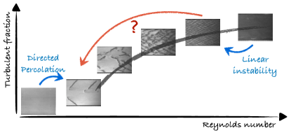
Here we tackle the remaining central issue illustrated in Fig. 1, namely how the strongly nonlinear evolution of the pattern leads, in a characteristic tipping evasion scenario Rietkerk et al. (2021), to the spatio-temporally intermittent regime when decreasing . Starting with the simplest two-fields model Manneville (2012), to which advection and noise are added, we reveal rich unexplored dynamics. More specifically, we show that (i) many stable patterns coexist with wave vectors delimited by the boundaries of the so-called Busse balloon Busse (1978), (ii) a specific wavelength is selected when adding a multiplicative noise that mimics the turbulent fluctuations, (iii) a cascade of instabilities lead to a dramatic increase of the wavelength on the lower side of the balloon, eventually reaching infinite wavelength, (iv) in this limit, the periodic limit cycle associated with the spatial pattern hits the laminar fixed point into a saddle-loop global bifurcation. According to this scenario, the pattern evolves from a regular harmonic pattern to a non-harmonic one, with a logarithmic divergence of its wavelength, while the turbulent regions remain essentially of constant size. The prediction compares well with existing data from the literature, as long as the pattern is well formed, i.e. before entering the spatio-temporal intermittent regime obeying the directed percolation scenario.
The Waleffe model Waleffe (1997); Dauchot and Vioujard (2000) was decisive in understanding the local self-sustaining process along which streamwise vortices () draw the mean flow () from high to low-velocity regions leading to streamwise velocity fluctuations called streaks (). The latter undergo an inflectional instability leading to modulations of amplitude (), feeding back the vortices and thereby sustaining turbulence. An important step forward was to propose a spatially extended version of the model including diffusive coupling Manneville (2012). Assuming fast dynamics for the fields and , the model was reduced to a two-field model, which exhibits a Turing linear instability of the homogeneous turbulent flow, when decreasing . Here we further expand on this first success by adding advection and a multiplicative noise to account for the fluctuating nature of the turbulent field . The model we study in one dimension then reads:
| (1a) | ||||
| (1b) | ||||
where are the diffusivities of the fields , is the amplitude of the noise and is a Gaussian random field with zero mean and (see Supp. Mat. sec. I-A,B for more details on the model ). The functions and are given by:
| (2a) | ||||
| (2b) | ||||
where the dependence on is encoded in the coefficients (see Supp. Mat. sec. I-B). The absorbing nature of the laminar state emerges from the form of and and is respected by the choice of a multiplicative noise.
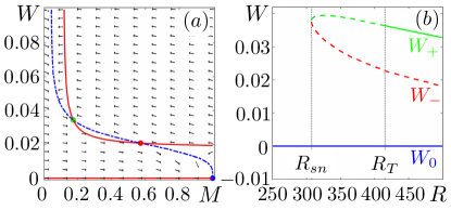
Figure 2 displays the vector field , together with the nullclines and , the intersection of which provide the spatially homogeneous fixed points. The laminar solution is linearly stable for all . For , two extra solutions emerge from a saddle node bifurcation. The lower branch is linearly unstable for all The parameter values are such that the upper branch is linearly stable with respect to homogeneous perturbations for , yet destabilizes via a Turing instability, when decreasing below (see also Dauchot and Vioujard (2000); Manneville (2012) and Supp. Mat. sec. I.C).
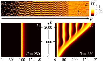
The simulation of Eqs. (1) with periodic boundary conditions in a domain of size (see Supp. Mat. sec. II-A) display the main features of the transitional regime in plane shear flows. When slowly annealing from the homogeneous turbulent state (Fig. 3-a), a periodic pattern emerges, the wavelength of which increases with decreasing . For low enough values of , the pattern is replaced by a disordered juxtaposition of isolated pulses, which eventually vanish when further decreasing below . For , the model exhibits an excitable-like behaviour: when initialized with a large enough amplitude Gaussian profile of , a localized pulse nucleates (Fig. 3-b). Single pulses, as well as superposition of multiple pulses, are stable. The amplitude of the initial condition necessary to trigger a pulse increases with decreasing . Nucleating two pulses one after the other either leads to a fusion of the two pulses when they are too close or to two distinct pulses, with the downstream one being pushed away from the upstream one. For , the initial Gaussian profile expands downstream, increasing the width between a laminar-turbulent front and a turbulent-laminar one. The turbulent state between the two fronts modulates, leading to a well-formed pattern (Fig. 3-c), as also seen in Alavyoon et al. (1986); Duguet et al. (2010).
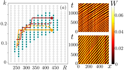
The pattern wavelength observed when applying the above annealing procedure is selected by noise. To show this, we first run deterministic simulations () with initial conditions in the form of a harmonically modulated turbulent state. We identify the stable patterns as those which keep the same wave number for very long times (). The region in the space encompassing all the stable patterns is called the Busse balloon (Busse, 1978). It extends for up to , retaining the subcriticality of the Turing instability reported in Manneville (2012), and down to , far below , in a characteristic evasion from the tipping point catastrophe Rietkerk et al. (2021). When initiating the noiseless simulation with a well-formed pattern and decreasing the Reynolds number, the wavelength remains constant until the pattern hits the left edge of the Busse balloon (continuous line trajectories on Fig. 4-a). Conversely, in the presence of noise, patterns initiated with two different wave numbers converge towards a narrow range of wavelength, which is also the one obtained when annealing from the homogeneous turbulent state (dashed line trajectories Fig. 4-a and spatio-temporal diagrams Fig. 4-b,c).
When , large wavelength patterns coexist with localized pulses in phase space. The connection between these two families of solutions is better described in the system of coordinate , where is the advection speed of the travelling solutions. One thereby obtains a 4-dimensional dynamical system:
| (3a) | ||||
| (3b) | ||||
| (3c) | ||||
| (3d) | ||||
with . The fixed points of this dynamical system are and are all saddles with two positive eigenvalues. The pattern and the pulse solutions of Eqs. (1) respectively map onto periodic orbits around the turbulent fixed point and homoclinic orbits of the laminar one (see Fig. 5-a). When reducing , the periodic orbits grow around the unstable homogeneous turbulent state (see Fig. 5-b), distort and approach the laminar saddle. The central question is whether a global saddle-loop bifurcation takes place, with the periodic orbits turning into homoclinic ones Strogatz (2000); Doelman et al. (2018). If such a scenario were to take place, it would strongly constrain the wavelength dependence on in the vicinity of the global bifurcation (Gaspard, 1990). This question can however not be answered using simulations with periodic boundary conditions, which formally only produce periodic solutions.
We thus turn to numerical continuation methods to follow the periodic orbits of Eqs. (3) and their stability Sherratt (2012) (see Sup. Mat. sec. II-B). A pattern solution at large , which advection speed is measured, is seeded as a solution for Eqs. (3). We then perform arc-length continuation, both increasing and decreasing , keeping fixed (black lines of Fig. 5-c,d), until a secondary bifurcation takes place (red and yellow bounds of Fig. 5,c-d). Starting from a stable solution, close to the lower instability, we then suggest a small increase in and iterate the procedure until the full Busse balloon, with a highly non-trivial shape at low , is obtained. In particular, we find two families of solutions with arbitrarily large periods located in the two ”legs”, resp. ”tips”, in the , resp. , representation of the Busse balloon. Those solutions eventually connect to the homoclinic orbits starting from the laminar fixed point and therefore confirm the global saddle-loop bifurcation scenario.
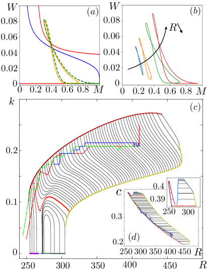
Fig. 5-(c,d) also displays the trajectory followed by the pattern solution in the and parameter spaces during three independent annealing processes as the one reported in Fig. 3-(a). The pattern selected by the noise at large moves across the Busse balloon, maintaining an essentially constant wavelength until it reaches its left boundary and follows it down to larger and larger wavelength. The growth of the wavelength is then controlled by the saddle-loop bifurcation and, therefore, obey the following logarithmic scaling Gaspard (1990):
| (4) |
with and where , with the critical value of , where the saddle-loop bifurcation takes place.
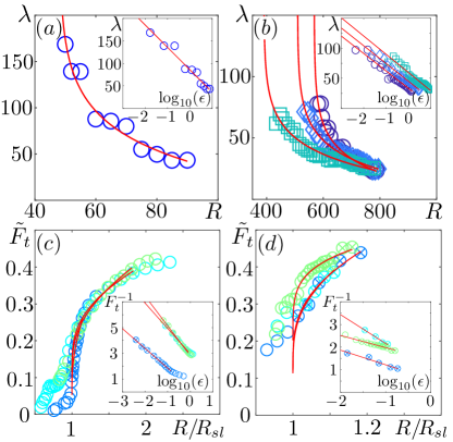
In real flows, the saddle-loop bifurcation scenario certainly does not strictly take place, first because of finite size effects and second because other mechanisms such as longitudinal band splitting Shimizu and Manneville (2019) may take over. Nevertheless, the proximity of a global bifurcation should control the behaviour of the wavelength in a critical regime for . We conclude this work by testing this hypothesis with existing experimental and numerical measurements of both the pattern wavelength and the turbulent fraction in plane Poiseuille flow (pPf) and TCf flows. The expected scaling of the turbulent fraction, , is obtained on the basis that the width of the turbulent bands is essentially constant in the vicinity of . In all cases, we find a remarkable agreement between the reported data and the scaling predicted in the proximity of a saddle-loop bifurcation (Eq. (4)). Note the deviation below , as the pattern breaks down and the other critical point for directed percolation is approached (see e.g Klotz et al. (2022)).
Altogether, the linear instability of the homogeneous turbulent flow leads to a plethora of coexisting metastable patterns, and the fluctuations select the wavelength of the observed nonlinear pattern. The limit cycle, associated with the selected wavelength, grows, distorts, and finally hits the laminar fixed point in a global saddle-loop bifurcation, leading to a logarithmic divergence of the wavelength and, as a consequence, of the turbulent fraction. In practice, the divergence is regularized by a crossover to richer dynamics involving more than one dimension. Nevertheless, the global bifurcation and the associated singularity control the dynamics in a critical range accessible experimentally and numerically. This calls for refined simulations and experiments in the vicinity of the crossover.
The present model shares some similarities with the two-fields one-dimensional model introduced in Barkley (2011) to describe the transition to turbulence in pipe flow. Both models describe excitable dynamics, allowing for stable localized pulse solutions corresponding to the turbulent spots. However, while in Barkley (2011) the inhibiting role of turbulence comes from an increased dissipation of the turbulent energy, here it arises from reduced turbulent energy production (see Supp. Mat. sec I.D). This is actually responsible for a structurally different organization of the vector field . In Barkley (2011), the nullclines have slopes of opposite signs when they cross, here the slopes have the same sign. This last property being a necessary condition for a Turing instability of the upper branch, Barkley (2011) does not exhibit laminar turbulent periodic patterns.
Finally, the scenario described above is not unique to the subcritical transition to turbulence. Reaction-diffusion is most common in many other contexts including biology, chemistry or ecology Turing (1952); Pearson (1993); Lengyel and Epstein (1992); Rietkerk et al. (2021) and generically leads to pattern formation via a linear instability, be the instability of strict Turing type or not. Making predictions beyond the weakly non-linear regime in such spatially extended systems is generally challenging. When the pattern wavelength increases away from the instability, the methodology presented here is a promising path to unveil the general scenario of a saddle-loop bifurcation Gaspard (1990); Plaza et al. (1997).
— Acknowledgments — PK acknowledges financial support from the French Ministry of Education and Research. We thank J.A. Sherratt for useful discussions on continuation methods. JFM thanks the support of the Competition for Research Regular Projects, year 2023, code LPR23-06, Universidad Tecnológica Metropolitana.
References
- Manneville (2015) P. Manneville, European Journal of Mechanics - B/Fluids 49, 345 (2015).
- Tuckerman et al. (2020) L. S. Tuckerman, M. Chantry, and D. Barkley, Annual Review of Fluid Mechanics 52, 343 (2020).
- Dauchot and Manneville (1997) O. Dauchot and P. Manneville, Journal de Physique II 7, 371 (1997), publisher: EDP Sciences.
- Pomeau (1986) Y. Pomeau, Physica D: Nonlinear Phenomena 23, 3 (1986).
- Lemoult et al. (2016) G. Lemoult, L. Shi, K. Avila, S. V. Jalikop, M. Avila, and B. Hof, Nature Physics 12, 254 (2016).
- Chantry et al. (2017) M. Chantry, L. S. Tuckerman, and D. Barkley, Journal of Fluid Mechanics 824, R1 (2017).
- Klotz et al. (2022) L. Klotz, G. Lemoult, K. Avila, and B. Hof, Physical Review Letters 128, 014502 (2022).
- Prigent et al. (2002) A. Prigent, G. Grégoire, H. Chaté, O. Dauchot, and W. van Saarloos, PRL 89, 014501 (2002).
- Prigent et al. (2003) A. Prigent, G. Grégoire, H. Chaté, and O. Dauchot, Physica D: Nonlinear Phenomena 174, 100 (2003).
- Tsukahara et al. (2014) T. Tsukahara, Y. Seki, H. Kawamura, and D. Tochio, “DNS of turbulent channel flow at very low Reynolds numbers,” (2014), arXiv:1406.0248 [physics].
- Duguet et al. (2010) Y. Duguet, P. Schlatter, and D. S. Henningson, Journal of Fluid Mechanics 650, 119 (2010).
- Ishida et al. (2016) T. Ishida, Y. Duguet, and T. Tsukahara, Journal of Fluid Mechanics 794, R2 (2016).
- Kunii et al. (2019) K. Kunii, T. Ishida, Y. Duguet, and T. Tsukahara, Journal of Fluid Mechanics 879, 579 (2019).
- Paranjape (2019) C. S. Paranjape, Ph.D. thesis, Institute of Science and Technology, Austria (2019).
- Shimizu and Manneville (2019) M. Shimizu and P. Manneville, Physical Review Fluids 4, 113903 (2019).
- Takeda and Tsukahara (2019) K. Takeda and T. Tsukahara, in Annual meeting of the Japanese society of fluid power (Tokyo, 2019).
- Kashyap et al. (2020) P. V. Kashyap, Y. Duguet, and O. Dauchot, Entropy 22, 1001 (2020).
- Moxey and Barkley (2010) D. Moxey and D. Barkley, Proceedings of the National Academy of Sciences 107, 8091 (2010).
- Tuckerman et al. (2008) L. S. Tuckerman, D. Barkley, and O. Dauchot, Journal of Physics: Conference Series 137, 012029 (2008).
- Kashyap et al. (2022) P. V. Kashyap, Y. Duguet, and O. Dauchot, Physical Review Letters 129, 244501 (2022).
- Manneville (2012) P. Manneville, EPL (Europhysics Letters) 98, 64001 (2012).
- Benavides and Barkley (2023) S. J. Benavides and D. Barkley, “Model for transitional turbulence in a planar shear flow,” (2023).
- Rietkerk et al. (2021) M. Rietkerk, R. Bastiaansen, S. Banerjee, J. van de Koppel, M. Baudena, and A. Doelman, Science 374, eabj0359 (2021).
- Busse (1978) F. H. Busse, Reports on Progress in Physics 41, 1929 (1978).
- Waleffe (1997) F. Waleffe, Physics of Fluids 9, 883 (1997).
- Dauchot and Vioujard (2000) O. Dauchot and N. Vioujard, The European Physical Journal B - Condensed Matter 14, 377 (2000).
- Alavyoon et al. (1986) F. Alavyoon, D. S. Henningson, and P. H. Alfredsson, Physics of Fluids 29, 1328 (1986).
- Strogatz (2000) S. H. Strogatz, Nonlinear Dynamics And Chaos: With Applications To Physics, Biology, Chemistry, And Engineering, 1st ed. (CRC Press, Cambridge, Mass, 2000).
- Doelman et al. (2018) A. Doelman, J. Rademacher, B. de Rijk, and F. Veerman, SIAM Journal on Applied Dynamical Systems 17, 1833 (2018).
- Gaspard (1990) P. Gaspard, The Journal of Physical Chemistry 94, 1 (1990).
- Sherratt (2012) J. A. Sherratt, Applied Mathematics and Computation 218, 4684 (2012).
- Prigent (2001) A. Prigent, Ph.D. thesis, Université Paris XI Orsay (2001).
- Barkley (2011) D. Barkley, Journal of Physics: Conference Series 318, 032001 (2011).
- Turing (1952) A. M. Turing, Philosophical Transactions of the Royal Society of London. Series B, Biological Sciences 237, 37 (1952).
- Pearson (1993) J. E. Pearson, Science 261, 189 (1993).
- Lengyel and Epstein (1992) I. Lengyel and I. R. Epstein, Proceedings of the National Academy of Sciences 89, 3977 (1992).
- Plaza et al. (1997) F. Plaza, M. Velarde, F. Arecchi, S. Boccaletti, M. Ciofini, and R. Meucci, Europhysics letters 38, 85 (1997).