Label Leakage and Protection in Two-party Split Learning
Abstract
Two-party split learning is a popular technique for learning a model across feature-partitioned data. In this work, we explore whether it is possible for one party to steal the private label information from the other party during split training, and whether there are methods that can protect against such attacks. Specifically, we first formulate a realistic threat model and propose a privacy loss metric to quantify label leakage in split learning. We then show that there exist two simple yet effective methods within the threat model that can allow one party to accurately recover private ground-truth labels owned by the other party. To combat these attacks, we propose several random perturbation techniques, including Marvell, an approach that strategically finds the structure of the noise perturbation by minimizing the amount of label leakage (measured through our quantification metric) of a worst-case adversary. We empirically demonstrate the effectiveness of our protection techniques against the identified attacks, and show that Marvell in particular has improved privacy-utility tradeoffs relative to baseline approaches.
1 Introduction
With increasing concerns over data privacy in machine learning, federated learning (FL) (McMahan et al., 2017) has become a promising direction of study. Based on how sensitive data are distributed among parties, FL can be classified into different categories, notable among which are horizontal FL and vertical FL (Yang et al., 2019). In contrast to horizontal FL where the data are partitioned by examples, vertical FL considers data partitioned by features (including labels). As a canonical example of vertical FL, consider an online media platform which displays advertisements from company to its users, and charges for each conversion (e.g., a user clicking the ad and buying the product). In this case, both parties have different features for each user: has features on the user’s media viewing records, while has the user’s conversion labels. ’s labels are not available to because each user’s purchase behaviors happen entirely on ’s website/app.
If both parties want to jointly learn a model to predict conversion without data sharing, split learning (Gupta and Raskar, 2018; Vepakomma et al., 2018) can be used to split the execution of a deep network between the parties on a layer-wise basis. In vanilla split learning, before training begins, both parties use Private Set Intersection (PSI) protocols (Kolesnikov et al., 2016; Pinkas et al., 2018) to find the intersection of their data records and achieve an example ID alignment. This alignment paves the way for the split training phase. During training (Figure 1), the party without labels (non-label party) sends the intermediate layer (cut layer) outputs rather than the raw data to the party with labels (label party), and the label party completes the rest of the forward computation to obtain the training loss. To compute the gradients with respect to model parameters, the label party initiates backpropagation from its training loss and computes its own parameters’ gradients. To allow the non-label party to also compute gradients of its parameters, the label party also computes the gradients with respect to the cut layer outputs and communicates this information back to the non-label party. As a result of the ID alignment, despite not knowing the label party’s raw label data, the non-label party can identify the gradient value returned by the label party for each example.

At first glance, the process of split learning appears privacy-preserving because only the intermediate computations of the cut layer—rather than raw features or labels—are communicated between the two parties. However, such “gradient sharing” schemes have been shown to be vulnerable to privacy leakage in horizontal FL settings (e.g., Zhu et al., 2019). In vertical FL (and specifically split learning), it remains unclear whether the raw data can similarly be leaked during communication. In particular, as the raw labels often contain highly sensitive information (e.g., what a user has purchased (in online advertising) or whether a user has a disease or not (in disease prediction) (Vepakomma et al., 2018)), developing a rigorous understanding of the threat of label leakage and its protection is particularly important. Towards this goal, we make the following contributions:
- 1.
-
2.
We identify two simple and realistic methods within this threat model which can accurately recover the label party’s private label information (Section 2).
-
3.
We propose several random perturbation techniques to limit the label-stealing ability of the non-label party (Section 4). Among them, our principled approach Marvell directly searches for the optimal random perturbation noise structure to minimize label leakage (as measured via our quantification metric) against a worst-case adversarial non-label party.
-
4.
We experimentally demonstrate the effectiveness of our protection techniques and Marvell’s improved privacy-utility tradeoffs compared to other protection baselines (Section 5).
2 Related Work
Privacy leakage in split learning. Although raw data is not shared in federated learning, sensitive information may still be leaked when gradients and/or model parameters are communicated between parties. In horizontal FL, Zhu et al. (2019) showed that an honest-but-curious server can uncover the raw features and labels of a device by knowing the model architecture, parameters, and communicated gradient of the loss on the device’s data. Based on their techniques, Zhao et al. (2020) showed that the ground truth label of an example can be extracted by exploiting the directions of the gradients of the weights connected to the logits of different classes. Here we study a different setting—two-party split learning (in vertical FL) (Yang et al., 2019), where no party has access to the model architecture or model parameters of the other party. In this setting, Vepakomma et al. (2019) studied how the forward communication of feature representations can leak the non-label party’s raw data to the label party. We instead study whether label information may be leaked from the label party to the non-label party during the backward communication. Despite the importance of maintaining the privacy of these labels, we are unaware of prior work that has studied this problem.
Privacy protection and quantification. Techniques to protect communication privacy in FL generally fall into three categories: 1) cryptographic methods such as secure multi-party computation (e.g., Bonawitz et al., 2017); 2) system-based methods including trusted execution environments (Subramanyan et al., 2017); and 3) perturbation methods that shuffle or modify the communicated messages (e.g., Abadi et al., 2016; McMahan et al., 2018; Erlingsson et al., 2019; Cheu et al., 2019; Zhu et al., 2019). Our protection techniques belong to the third category, as we add random perturbations to the gradients to protect the labels. Many randomness-based protection methods have been proposed in the domain of horizontal FL. In this case, differential privacy (DP) (Dwork, 2006; Dwork et al., 2014) is commonly used to measure the proposed random mechanisms’ ability to anonymize the identity of any single participating example in the model iterates. However, in split learning, after PSI, both parties know exactly the identity of which example has participated in a given gradient update. As we explain in Section 3.1, the object we aim to protect (the communicated cut layer gradients), unlike the model iterates, is not an aggregate function of all the examples but are instead example-specific. As a result, DP and its variants (e.g. label DP (Chaudhuri and Hsu, 2011; Ghazi et al., 2021)) are not directly applicable metrics in our setting, and we instead propose a different metric (discussed in Section 3.2).
3 Label Leakage in Split Learning
We first introduce the two-party split learning problem for binary classification, and then formally describe our threat model and privacy quantification metrics with two concrete attack examples.
3.1 Two-party Split Learning in Binary Classification
Problem setup. Consider two parties learning a composition model jointly for a binary classification problem over the domain (Figure 1). The non-label party owns the representation function and each example’s raw feature while the label party owns the logit function and each example’s label 111 To simplify notation, we assume no additional features in the label party to compute the logit. The data leakage problem still holds true for other more complicated settings (see WDL experiment setting in Section 5). . Let be the logit of the positive class whose predicted probability is given through the sigmoid function: . We measure the loss of such prediction through the cross entropy loss . During model inference, the non-label party computes and sends it to the label party who will then execute the rest of forward computation in Figure 1.
Model training (Figure 1: backward gradient computation). To train the model using gradient descent, the label party starts by first computing the gradient of the loss with respect to the logit . Using the chain rule, the label party can then compute the gradient of with respect to its function ’s parameters and perform the gradient updates. To also allow the non-label party to learn its function , the label party needs to additionally compute the gradient with respect to cut layer feature and communicate it to the non-label party. We denote this gradient by (by chain rule). After receiving , the non-label party continues the backpropagation towards ’s parameters and also perform the gradient updates.
Why Not Differential Privacy? Note that for a given iteration, the non-label party randomly chooses example IDs to form a batch. Therefore, the identity of which examples are used is known to the non-label party by default. In addition, the communicated features and returned gradients will both be matrices in with each row belonging to a specific example in the batch. The different gradients (rows of the matrix) are not with respect to the same model parameters, but are instead with respect to different examples’ cut-layer features; thus, no averaging over or shuffling of the rows of the gradient matrix can be done prior to communication to ensure correct computation of ’s parameters on the non-label party side. This example-aware and example-specific nature of the communicated gradient matrix makes differential privacy (which focuses on anonymizing an example’s participation in an aggregate function) inapplicable for this problem (see also Section 2).
3.2 Threat Model and Privacy Quantification
Below we specify several key aspects of our threat model, including the adversary’s objective and capabilities, our metric for quantifying privacy loss, and the possible inclusion of side information.
Adversary’s objective. At a given moment in time during training (with and fixed), since the communicated cut layer gradient is a deterministic function of and (see Section 3.1), we consider an adversarial non-label party whose objective is to recover the label party’s hidden label based on the information contained in for every training example.
Adversary’s capability. We consider an honest-but-curious non-label party which cannot tamper with training by selecting which examples to include in a batch or sending incorrect features ; instead, we assume that the adversary follows the agreed-upon split training procedure while trying to guess the label . This can be viewed as a binary classification problem where the (input, output) distribution is the induced distribution of . We allow the adversary to use any binary classifier to guess the labels. This classifier can be represented by a (scoring function , threshold ) tuple, where maps an example’s cut layer gradient to a real-valued score and the threshold determines a cut-off so that if and if . Moving forward, we use this tuple representation to describe adversarial non-label party classifiers.
Privacy loss quantification. As we consider binary classification, a natural metric to quantify the performance of an adverary’s scoring function is the AUC of its ROC curve. Denote the unperturbed class-conditional distributions of the cut-layer gradients by and for the positive and negative class, respectively. The ROC curve of a scoring function is a parametric curve which maps a threshold value to the corresponding (False Positive Rate, True Positive Rate) tuple of the classifier represented by , with and . The AUC of the ROC curve of a scoring function (denote by ) can be expressed as an integral:
| (Leak AUC) |
(more details on this expression see Appendix A.1.) We use this value as the privacy loss quantification metric for a specific adversary scoring function and refer to it as the leak AUC. This metric summarizes the predictive performance of all classifiers that can be constructed through all threshold values and removes the need to tune this classifier-specific hyperparameter. The leak AUC being close to implies that the corresponding scoring function can very accurately recover the private label, whereas a value of around means is non-informative in predicting the labels. In practice, during batch training, the leak AUC of can be estimated at every gradient update iteration using the minibatch of cut-layer gradients together with their labels.
Side information. Among all the scoring functions within our threat model, it is conceivable that only some would recover the hidden labels more accurately than others and thus achieve a higher value of leak AUC. Picking these effective scoring functions would require the non-label party to have population-level side information specifically regarding the properties of (and distinction between) the positive and negative class’s cut-layer gradient distributions. Because we allow the adversary to pick any specific (measurable) scoring function , we implicitly allow for such population-level side information for the adversary. However, we assume the non-label party has no example-level side information that is different example by example. Next we provide two scoring function examples which use population-level side-information to effectively recover the label .
3.3 Practical Attack Methods
(a)

(b)

(c)

(d)

(e)

Attack 1: Norm-based scoring function. Note that . We make the following observations for and , which hold true for a wide range of real-world learning problems.
-
•
Observation 1: Throughout training, the model tends to be less confident about a positive example being positive than a negative example being negative. In other words, the confidence gap of a positive example (when ) is typically larger than the confidence gap of a negative example (when ) (see Figure 2(a)). This observation is particularly true for problems like advertising conversion prediction and disease prediction, where there is inherently more ambiguity for the positive class than the negative. For example, in advertising, uninterested users of a product will never click on its ad and convert, but those interested, even after clicking, might make the purchase only a fraction of the time depending on time/money constraints. (See a toy example of this ambiguity in the Appendix A.2.)
-
•
Observation 2: Throughout training, the norm of the gradient vector is on the same order of magnitude (has similar distribution) for both the positive and negative examples (Figure 2(b)). This is natural because is not a function of .
As a consequence of Observation 1 and 2, the gradient norm of the positive instances are generally larger than that of the negative ones (Figure 2(c)). Thus, the scoring function is a strong predictor of the unseen label . We name the privacy loss (leak AUC) measured against the attack the norm leak AUC. In Figure 2(c), the norm leak AUCs are consistently above , signaling a high level of label leakage throughout training.
Attack 2: Direction-based scoring function. We now show that the direction of (in addition to its length) can also leak the label. For a pair of examples, , let their respective predicted positive class probability be , and their communicated gradients be , . Let denote the cosine similarity function . It is easy to see that , where sgn(x) is the sign function which returns if , and if . We highlight two additional observations that can allow us to use cosine similarity to recover the label.
-
•
Observation 3: When the examples are of different classes, the term is negative. On the other hand, when examples , are of the same class (both positive/both negative), this product will have a value of and thus be positive.
-
•
Observation 4: Throughout training, for any two examples , their gradients of the function always form an acute angle, i.e. (Figure 2(d)). For neural networks that use monotonically increasing activation functions (such as ReLU, sigmoid, ), this is caused by the fact that the gradients of these activation functions with respect to its inputs are coordinatewise nonnegative and thus always lie in the first closed hyperorthant.
Since is the product of the terms from Observation 3 and 4, we see that for a given example, all the examples that are of the same class result in a positive cosine similarity, while all opposite class examples result in a negative cosine similarity. If the problem is class-imbalanced and the non-label party knows there are fewer positive examples than negative ones, it can thus determine the label of each example: the class is negative if more than half of the examples result in positive cosine similarity; otherwise it is positive. For many practical applications, the non-label party may reasonably guess which class has more examples in the dataset a priori without ever seeing any data—for example, in disease prediction, the percentage of the entire population having a certain disease is almost always much lower than 50%; in online advertising conversion prediction, the conversion rate (fraction of positive examples) is rarely higher than 30%. Note that the non-label party doesn’t need knowledge of the exact sample proportion of each class for this method to work.
To simplify this attack for evaluation, we consider an even worse oracle scenario where the non-label party knows the clean gradient of one positive example . Unlike the aforementioned practical majority counting attack which needs to first figure out the direction of one positive gradient, this oracle scenario assumes the non-label party is directly given this information. Thus, any protection method capable of defending this oracle attack would also protect against the more practical one. With given, the direction-based scoring function is simply . We name the privacy loss (leak AUC) against this oracle attack the cosine leak AUC. In practice, we randomly choose a positive class clean gradient from each batch as for evaluation. For iterations in Figure 2(e), the cosine leak AUC all have the highest value of (complete label leakage).
4 Label Leakage Protection Methods
In this section, we first introduce a heuristic random perturbation approach designed to prevent the practical attacks identified in Section 2. We then propose a theoretically justified method that aims to protect against the entire class of scoring functions considered in our threat model (Section 3.2).
4.1 A Heuristic Protection Approach
Random perturbation and the isotropic Gaussian baseline. To protect against label leakage, the label party should ideally communicate essential information about the gradient without communicating its actual value. Random perturbation methods generally aim to achieve this goal. One obvious consideration for random perturbation is to keep the perturbed gradients unbiased. In other words, suppose is the perturbed version of an example’s true gradient , then we want . By chain rule and linearity of expectation, this ensures the computed gradients of the non-label party’s parameters will also be unbiased, a desirable property for stochastic optimization. Among unbiased perturbation methods, a simple approach is to add iid isotropic Gaussian noise to every gradient to mix the positive and negative gradient distribution before sending to the non-label party. Although isotropic Gaussian noise is a valid option, it may not be optimal because 1) the gradients are vectors but not scalars, so the structure of the noise covariance matrix matters. Isotropic noise might neglect the direction information; 2) due to the asymmetry of the positive and negative gradient distribution, the label party could add noise with different distributions to each class’s gradients.
Norm-alignment heuristic. We now introduce an improved heuristic approach of adding zero-mean Gaussian noise with non-isotropic and example-dependent covariance. [Magnitude choice] As we have seen that can be different for positive and negative examples and thus leak label information, this heuristic first aims to make the norm of each perturbed gradient indistinguishable from one another. Specifically, we want to match the expected squared -norm of every perturbed gradient in a mini-batch to the largest squared -norm in this batch (denote by ). [Direction choice] In addition, as we have seen empirically from Figure 2(e), the positive and negative gradients lie close to a one-dimensional line in , with positive examples pointing in one direction and negative examples in the other. Thus we consider only adding noise (roughly speaking) along “this line”. More concretely, for a gradient in the batch, we add a zero-mean Gaussian noise vector supported only on the one-dimensional space along the line of . In other words, the noise’s covariance is the rank- matrix . To calculate , we aim to match . A simple calculation gives . Since we align to the maximum norm, we name this heuristic protection method max_norm. The advantage of max_norm is that it has no parameter to tune. Unfortunately, it does not have a strong theoretical motivation, cannot flexibly trade-off between model utility and privacy, and may be broken by some unknown attacks.
4.2 Optimized Perturbation Method: Marvell
Motivated by the above issues of max_norm, we next study how to achieve a more principled trade-off between model performance (utility) and label protection (privacy). To do so, we directly minimize the worst-case adversarial scoring function’s leak AUC under a utility constraint. We name this protection method Marvell (optiMized perturbAtion to pReVEnt Label Leakage).
Noise perturbation structure. Due to the distribution difference between the positive and negative class’s cut layer gradients, we consider having the label party additively perturb the randomly sampled positive and negative gradients with independent zero-mean random noise vectors and with possibly different distributions (denoted by and ). We use and to denote the induced perturbed positive and negative gradient distributions. Our goal is to find the optimal noise distributions and by optimizing our privacy objective described below.
Privacy protection optimization objective. As the adversarial non-label party in our threat model is allowed to use any measurable scoring function for label recovery, we aim to protect against all such scoring functions by minimizing the privacy loss of the worst case scoring function measured through our leak AUC metric. Formally, our optimization objective is . Here to compute , the and needs to be computed using the perturbed distributions and instead of the unperturbed and (Section 3.2). Since AUC is difficult to directly optimize, we consider optimizing an upper bound through the following theorem:
Theorem 1.
For and any perturbed gradient distributions and that are absolutely continuous with respect to each other,
implies .
From Theorem 1 (proof in Appendix A.3), we see that as long as the sum KL divergence is below , the smaller sumKL is, the smaller is. ( decreases as decreases.) Thus we can instead minimize the sum KL divergence between the perturbed gradient distributions:
| (1) |
Utility constraint. In an extreme case, we could add infinite noise to both the negative and positive gradients. This would minimize (1) optimally to and make the worst case leak AUC , which is equivalent to a random guess. However, stochastic gradient descent cannot converge under infinitely large noise, so it is necessary to control the variance of the added noise. We thus introduce the noise power constraint: , where is the fraction of positive examples (already known to the label party); denotes the trace of the covariance matrix of the random noise ; and the upper bound is a tunable hyperparameter to control the level of noise: larger would achieve a lower sumKL and thus lower worst-case leak AUC and better privacy; however, it would also add more noise to the gradients, leading to slower optimization convergence and possibly worse model utility. We weight each class’s noise level by its example proportion ( or ) since, from an optimization perspective, we want to equally control every training example’s gradient noise. The constrained optimization problem becomes:
| (2) |
Optimizing the objective in practice. To solve the optimization problem we first introduce some modelling assumptions. We assume that the unperturbed gradient of each class follows a Gaussian distribution: and . Despite this being an approximation, as we see later in Section 5, it can achieve strong protection quality against our identified attacks. In addition, it makes the optimization easier (see below) and provides us with insight on the optimal noise structure. We also search for perturbation distributions that are Gaussian: and with commuting covariance matrices: . The commutative requirement slightly restricts our search space but also makes the optimization problem more tractable. Our goal is to solve for the optimal noise structure, i.e. the positive semidefinite covariance matrices , . Let denote the difference between the positive and negative gradient’s mean vectors. We now have the following theorem (proof and interpretation in Appendix A.4):
Theorem 2.
The optimal and to (2) with the above assumptions have the form:
| (3) |
where is the solution to the following 4-variable optimization problem:
| s.t. | |||
Additional details of Marvell. By Theorem 2, our optimization problem over two positive semidefinite matrices is reduced to a much simpler 4-variable optimization problem. We include a detailed description of how the constants in the problem are estimated in practice and what solver we use in a full description of the Marvell algorithm in Appendix LABEL:appsubsec:marvell_details. Beyond optimization details, it is worth noting how to set the power constraint hyperparameter in Equation 2 in practice. As directly choosing requires knowledge of the scale of the gradients in the specific application and the scale could also shrink as the optimization converges, we instead express , and tune for a fixed hyperparameter . This alleviates the need to know the scale of the gradients in advance, and the resulting value of can also dynamically change throughout training as the distance between the two gradient distributions’ mean changes.
5 Experiments
In this section, we first describe our experiment setup and then demonstrate the label protection quality of Marvell as well as its privacy-utility trade-off relative to baseline approaches.
Empirical Setup. We use three real-world binary classification datasets for evaluation: Criteo and Avazu , two online advertising prediction datasets with millions of examples; and ISIC , a healthcare image dataset for skin cancer prediction. All datasets are naturally imbalanced, making the label leakage problem more severe (see Appendix LABEL:appsubsubsec:dataset_preprocessing on dataset and preprocessing details). We defer similar results on Avazu to Appendix LABEL:appsubsec:experiment_results and focus on Criteo and ISIC in this section. For Criteo, we train a Wide&Deep model (Cheng et al., 2016) where the non-label party owns the embedding layers for input features and the first three -unit ReLU activated MLP layers (first half of the deep part) while the label party owns the remaining layers of the deep part and the entire wide part of the model222In this setting, the label party will also process input features (through the wide part) just like the non-label party, further relaxing our formal split learning setup in Section 3.. For ISIC, we train a model with 6 convolutional layers each with 64 channels followed by a 64-unit ReLU MLP layer, and the cut layer is after the fourth convolutional layer. In this case, an example’s cut layer feature and gradient are both in . We treat such tensors as vectors in to fit into our analysis framework (for additional model architecture and training details see Appendix LABEL:appsubsubsec:model_architecture, LABEL:appsubsubsec:model_training_details).
5.1 Label Leakage and Marvell’s Strong and Flexible Protection
We first evaluate the protection quality of Marvell against the norm and cosine attacks discussed in Section 2. We also compare against the leakage metrics when no protection is applied (no_noise). As the results across the three datasets are highly similar, we use ISIC as an example (other datasets see Appendix LABEL:app:subsubsec_leakauc_progression). We see in Figure 3(a)(b) that unlike no_noise where the label information is completely leaked (leak AUC ) throughout training, Marvell achieves a flexible degree of protection (by varying ) against both the norm 2(a) and direction attacks 2(b) on the cut layer gradients and has strong protection (leak AUC 0.5) at . Additionally, it is natural to ask whether the gradients of layers before the cut layer (on the non-label party side) can also leak the labels as the non-label party keeps back propagating towards the first layer. In Figure 3(c)(d), we compute the leak AUC values when using the non-label party’s first layer activation gradient as inputs to the scoring functions to predict . Without protection, the first layer gradient still leaks the label very consistently. In constrast, Marvell still achieves strong privacy protection at the first layer () despite the protection being analyzed at the cut layer.

5.2 Privacy-Utility Trade-off Comparison
After showing Marvell can provide strong privacy protection against our identified attacks, we now see how well it can preserve utility by comparing its privacy-utility tradeoff against other protection baselines: no_noise, isotropic Gaussian (iso), and our proposed heuristic max_norm. Similar to how we allow Marvell to use a power constraint to depend on the current iteration’s gradient distribution through , we also allow iso to have such type of dependence—specifically, we add to every gradient in a batch with a tunable privacy hyperparameter to be fixed throughout training. To trace out the complete tradeoff curve for Marvell and iso, we conduct more than 20 training runs for each protection method with a different value of privacy hyperparameter ( for Marvell, for iso) in each run on every dataset. (Note that no_noise and max_norm do not have privacy hyperparameters.)
We present the tradeoffs between privacy (measured through norm and cosine leak AUC at cut layer/first layer) and utility (measured using test loss and test AUC) in Figure 4. To summarize the leak AUC over a given training run, we pick the 95% quantile over the batch-computed leak AUCs throughout all training iterations. This quantile is chosen instead of the mean because we want to measure the most-leaked iteration’s privacy leakage (highest leak AUC across iterations) to ensure the labels are not leaked at any points during training. quantile is chosen instead of the max () as we want this privacy leak estimate to be robust against randomness of the training process.


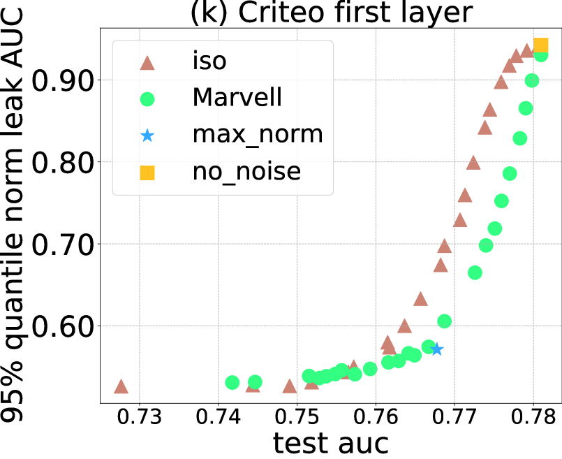

Privacy-Utility Tradeoff comparison results. In measuring the privacy-utility tradeoff, we aim to find a method that consistently achieves a lower leak AUC (better privacy) for the same utility value.
-
•
[Marvell vs iso] As shown in Figure 4, Marvell almost always achieves a better tradeoff than iso against both of our proposed attacks at both the cut layer and the first layer on both the ISIC and Criteo datasets. It is important to note that although the utility constraint is in terms of training loss optimization, Marvell’s better tradeoff still translates to the generalization performance when the utility is measured through test loss or test AUC. Additionally, despite achieving reasonable (though still worse than Marvell) privacy-utility tradeoff against the norm-based attack, iso performs much worse against the direction-based attack: on ISIC, even after applying a significant amount of isotropic noise (with ), iso’s cosine leak AUC is still higher than at the cut layer (Figure 4(b,f)). In contrast, Marvell is effective against this direction-based attack with a much lower cosine leak AUC .
-
•
[max_norm heuristic] Beyond Marvell, we see that our heuristic approach max_norm can match and sometimes achieve even lower (Figure 4(a,f,i)) leak AUC value than Marvell at the same utility level. We believe this specifically results from our norm and direction consideration when designing this heuristic. However, without a tunable hyperparameter, max_norm cannot tradeoff between privacy and utility. Additionally, unlike Marvell which is designed to protect against the entire class of adversarial scoring functions, max_norm might still fail to protect against other future attack methods beyond those considered here.
In summary, our principled method Marvell significantly outperforms the isotropic Gaussian baseline, and our proposed max_norm heuristic can also work particularly well against the norm- and direction-based attacks which we identified in Section 2.
6 Conclusion
In this paper, we formulate a label leakage threat model in the two-party split learning binary classification problem through a novel privacy loss quantification metric (leak AUC). Within this threat model, we provide two simple yet effective attack methods that can accurately uncover the private labels of the label party. To counter such attacks, we propose a heuristic random perturbation method max_norm as well as a theoretically principled method Marvell which searches for the optimal noise distributions to protect against the worst-case adversaries in the threat model. We have conducted extensive experiments to demonstrate the effectiveness of Marvell and max_norm over the isotropic Gaussian perturbation baseline iso.
Open questions and future work. Our work is the first we are aware of to identify, rigorously quantify, and protect against the threat of label leakage in split-learning, and opens up a number of worthy directions of future study. In particular, as the model parameters are updated every batch in our problem setup, the true gradient of an example and the gradient distribution would both change. An interesting question is whether the adversarial non-label party can remember the stale gradient of the same example from past updates (possibly separated by hundreds of updates steps) in order to recover the label information in the current iteration in a more complex threat model. It would also be interesting to build on our results to study whether there exist attack methods when the classification problem is multiclass instead of binary, and when the split learning scenario involves more than two parties with possibly more complicated training communication protocols (e.g., Vepakomma et al., 2018).
References
- McMahan et al. [2017] Brendan McMahan, Eider Moore, Daniel Ramage, Seth Hampson, and Blaise Aguera y Arcas. Communication-efficient learning of deep networks from decentralized data. In Artificial Intelligence and Statistics, pages 1273–1282. PMLR, 2017.
- Yang et al. [2019] Qiang Yang, Yang Liu, Tianjian Chen, and Yongxin Tong. Federated machine learning: Concept and applications. ACM Transactions on Intelligent Systems and Technology (TIST), 10(2):1–19, 2019.
- Gupta and Raskar [2018] Otkrist Gupta and Ramesh Raskar. Distributed learning of deep neural network over multiple agents. Journal of Network and Computer Applications, 116:1–8, 2018.
- Vepakomma et al. [2018] Praneeth Vepakomma, Otkrist Gupta, Tristan Swedish, and Ramesh Raskar. Split learning for health: Distributed deep learning without sharing raw patient data. arXiv preprint arXiv:1812.00564, 2018.
- Kolesnikov et al. [2016] Vladimir Kolesnikov, Ranjit Kumaresan, Mike Rosulek, and Ni Trieu. Efficient batched oblivious prf with applications to private set intersection. In Proceedings of the 2016 ACM SIGSAC Conference on Computer and Communications Security, CCS ’16, page 818–829, 2016.
- Pinkas et al. [2018] Benny Pinkas, Thomas Schneider, and Michael Zohner. Scalable private set intersection based on ot extension. ACM Transactions on Privacy and Security (TOPS), 21(2):1–35, 2018.
- Zhu et al. [2019] Ligeng Zhu, Zhijian Liu, and Song Han. Deep leakage from gradients. In Advances in Neural Information Processing Systems, pages 14774–14784, 2019.
- Zhao et al. [2020] Bo Zhao, Konda Reddy Mopuri, and Hakan Bilen. idlg: Improved deep leakage from gradients. arXiv preprint arXiv:2001.02610, 2020.
- Vepakomma et al. [2019] Praneeth Vepakomma, Otkrist Gupta, Abhimanyu Dubey, and Ramesh Raskar. Reducing leakage in distributed deep learning for sensitive health data. arXiv preprint arXiv:1812.00564, 2019.
- Bonawitz et al. [2017] Keith Bonawitz, Vladimir Ivanov, Ben Kreuter, Antonio Marcedone, H Brendan McMahan, Sarvar Patel, Daniel Ramage, Aaron Segal, and Karn Seth. Practical secure aggregation for privacy-preserving machine learning. In Proceedings of the 2017 ACM SIGSAC Conference on Computer and Communications Security, pages 1175–1191, 2017.
- Subramanyan et al. [2017] Pramod Subramanyan, Rohit Sinha, Ilia Lebedev, Srinivas Devadas, and Sanjit A Seshia. A formal foundation for secure remote execution of enclaves. In Proceedings of the 2017 ACM SIGSAC Conference on Computer and Communications Security, pages 2435–2450, 2017.
- Abadi et al. [2016] Martin Abadi, Andy Chu, Ian Goodfellow, H Brendan McMahan, Ilya Mironov, Kunal Talwar, and Li Zhang. Deep learning with differential privacy. In Proceedings of the 2016 ACM SIGSAC Conference on Computer and Communications Security, pages 308–318, 2016.
- McMahan et al. [2018] H. Brendan McMahan, Daniel Ramage, Kunal Talwar, and Li Zhang. Learning differentially private recurrent language models. In International Conference on Learning Representations, 2018. URL https://openreview.net/forum?id=BJ0hF1Z0b.
- Erlingsson et al. [2019] Úlfar Erlingsson, Vitaly Feldman, Ilya Mironov, Ananth Raghunathan, Kunal Talwar, and Abhradeep Thakurta. Amplification by shuffling: From local to central differential privacy via anonymity. In Proceedings of the Thirtieth Annual ACM-SIAM Symposium on Discrete Algorithms, pages 2468–2479. SIAM, 2019.
- Cheu et al. [2019] Albert Cheu, Adam Smith, Jonathan Ullman, David Zeber, and Maxim Zhilyaev. Distributed differential privacy via shuffling. In Annual International Conference on the Theory and Applications of Cryptographic Techniques, pages 375–403. Springer, 2019.
- Dwork [2006] Cynthia Dwork. Differential privacy. In Michele Bugliesi, Bart Preneel, Vladimiro Sassone, and Ingo Wegener, editors, Automata, Languages and Programming, pages 1–12, Berlin, Heidelberg, 2006. Springer Berlin Heidelberg. ISBN 978-3-540-35908-1.
- Dwork et al. [2014] Cynthia Dwork, Aaron Roth, et al. The algorithmic foundations of differential privacy. Foundations and Trends in Theoretical Computer Science, 9(3-4):211–407, 2014.
- Chaudhuri and Hsu [2011] Kamalika Chaudhuri and Daniel Hsu. Sample complexity bounds for differentially private learning. In Proceedings of the 24th Annual Conference on Learning Theory, pages 155–186. JMLR Workshop and Conference Proceedings, 2011.
- Ghazi et al. [2021] Badih Ghazi, Noah Golowich, Ravi Kumar, Pasin Manurangsi, and Chiyuan Zhang. On deep learning with label differential privacy. arXiv preprint arXiv:2102.06062, 2021.
- [20] Criteo. Criteo display advertising challenge, 2014. URL https://www.kaggle.com/c/criteo-display-ad-challenge/data.
- [21] Avazu. Avazu click-through rate prediction, 2015. URL https://www.kaggle.com/c/avazu-ctr-prediction/data.
- [22] ISIC. Siim-isic melanoma classification, 2020. URL https://www.kaggle.com/c/siim-isic-melanoma-classification/data.
- Cheng et al. [2016] Heng-Tze Cheng, Levent Koc, Jeremiah Harmsen, Tal Shaked, Tushar Chandra, Hrishi Aradhye, Glen Anderson, Greg Corrado, Wei Chai, Mustafa Ispir, et al. Wide & deep learning for recommender systems. In Proceedings of the 1st workshop on deep learning for recommender systems, pages 7–10, 2016.
Appendix A Appendix
A.1 Expressing as an integral
Recall that the ROC curve of a scoring function is a parametric curve such that , with
We notice that and are both monotonically decreasing functions in with
However, and does not need to be differentiable everywhere with respect to . Thus we cannot simply express the area under the curve using . On the other hand, because both and are functions of bounded variations, we can express the area under the parametric curve through the Riemann-Stieltjes integral which involves integrating the function with respect to the function :
Here the integration boundary is from to in order to ensure the integral evaluates to a positive value.
A.2 Toy example of positive example prediction lacking confidence
As mentioned in Observation 1 of norm-based attack in Section 2, for many practical applications, there is inherently more ambiguity for the positive class than the negative class. To make this more concrete, let’s consider a simple toy example.
Suppose the binary classification problem is over the real line. Here, 50% of the data is positive and lies uniformly in the interval . On the other hand, the remaining negative data (the other 50% of the total data) is a mixture distribution: 10% of the negative data also lies uniformly in , while the rest 90% of the negative data lies uniformly in .
This setup mirrors our online advertising example where for all the users interested in the product (with feature ), only a part of them would actually make the purchase after clicking on its advertisement.
In this case, the best possible probabilistic classifiers that can be ever learned, by Bayes Rule, would predict any example in to be of the positive class with probability , while it would predict any example in to be of the negative class with probability :
Thus even for this best possible classifier , every positive example would have a confidence gap of while of the negative examples (the ones in ) would have a confidence gap of . Hence we see that in this toy example, our empirical observation of the lack of prediction confidence for positive examples would still hold true.
Besides, it is important to notice that this lack of positive prediction confidence phenomenon happens even in this class-balanced toy example (). Thus, Observation 1 does not require the data distribution to be class-imbalanced to hold, which further demonstrates the generality of our norm-based attack.
A.3 Proof of Theorem 1
Theorem 1.
For and any perturbed gradient distributions and that are absolutely continuous with respect to each other,
Proof of Theorem 1.
Combining Pinsker’s inequality with Jensen’s inequality, we can obtain an upper bound of total variation distance by the symmetrized KL divergence (sumKL) for a pair of distributions that are absolutely continuous with respect to each other:
| (4) |
By our assumption, this implies that . By the equivalent definition of total variation distance , we know that for any , . For any scoring function and any threshold value , let , then we have .
Therefore, the AUC of the scoring function can be upper bounded in the following way:
| (5) | ||||
| (6) |
where in (6) we use the additional fact that for all .
When , we have . As is a monotonically nonincreasing function in with range in , the set is not empty. Let . Again by being a monotonically nonincreasing function in , we can break the integration in Equation (6) into two terms:
| (7) | ||||
| (8) | ||||
| (9) | ||||
| (10) | ||||
| (11) |
Since this inequality is true for any scoring function , it is true for the maximum value. Thus the proof is complete. ∎
A.4 Proof and Interpretation of Theorem 2
Theorem 2.
The optimal and to the following problem
have the form:
| (12) |
where is the solution to the following 4-variable optimization problem:
| s.t. | |||
Proof of Theorem 2.
By writing out the analytical close-form of the KL divergence between two Gaussian distributions, the optimization can be written as:
| (13) | ||||
By the commutative constraint on the two positive semidefinite matrices and , we know that we can factor these two matrices using the same set of eigenvectors. We thus write:
| (14) |
where is an orthogonal matrix and the eigenvalues are nonnegative and decreasing in value.
Using this alternative expression of and , we can express the optimization in terms of :
For any fixed feasible , we see that the corresponding minimizing will set its first row to be the unit vector in the direction of . Thus by first minimizing , the optimization objective reduces to:
We see that for the pair of variable (), the function is strictly convex over the line segment for any nonnegative and attains the the minimum value at when and when . Suppose without loss of generality , then for the optimal solution we must have for all . Under this condition, we notice that the function is strictly convex on the positive reals. Thus for all that satisfies for a fixed nonnegative , by Jensen inequality, we have
From this, we see that the optimal solution’s variables must take on the same value () for all . The case when is similar. As a result, we have proved that at the optimal solution, we must have:
Hence, the optimization problem over the variables can be reduced to an optimization problem over the four variables :
| (15) | ||||
Given the optimal solution to the above 4-variable problem , we can set to be any orthogonal matrix whose first row is the vector . Plugging this back into the expression of and in Equation (14) gives us the final result.
Thus the proof is complete. ∎
Remark (Interpreting the optimal and ).
From the form of the optimal solution in (12), we see that the optimal covariance matrices are both linear combinations of two terms: a rank one matrix and the identity matrix . Because a zero-mean Gaussian random vector with convariance matrix can be constructed as the sum of two independent zero-mean Gaussian random vectors with covariance matrices and respectively, we see that the optimal additive noise random variables and each consist of two independent components: one random component lies along the line that connects the positive and negative gradient mean vectors (whose covariance matrix is proportional to ); the other component is sampled from an isotropic Gaussian. The use of the first random directional component and the fact that the isotropic Gaussian component have different variance scaling for the positive and negative class clearly distinguishes Marvell from the isotropic Gaussian baseline iso.