Koopman embedding and super-linearization counterexamples with isolated equilibria
Abstract.
A frequently repeated claim in the “applied Koopman operator theory” literature is that a dynamical system with multiple isolated equilibria cannot be linearized in the sense of admitting a smooth embedding as an invariant submanifold of a linear dynamical system. This claim is sometimes made only for the class of super-linearizations, which additionally require that the embedding “contain the state”. We show that both versions of this claim are false by constructing (super-)linearizable smooth dynamical systems on having any countable (finite) number of isolated equilibria for each .
2020 Mathematics Subject Classification:
Primary 37C15A linearizing embedding of a nonlinear smooth dynamical system is a global identification of the nonlinear system with an invariant submanifold of a linear dynamical system. Linearizing embeddings have been studied by various communities and are of central importance in the rapidly developing “applied Koopman operator theory” literature [BBKK22]. An oft-repeated claim in that literature is that any dynamical system with multiple isolated equilibria cannot be linearized by a smooth embedding, or at least not by an embedding that “contains the state”. We call the latter type of linearizing embeddings super-linearizations.
The first claim was shown to be false by the authors in [KA23, Ex. 4] if non-Euclidean state spaces are allowed. In the present paper we show that both claims are also false for Euclidean state spaces by constructing for each (i) linearizable dynamical systems on having any countable number of isolated equilibria and (ii) super-linearizable dynamical systems on having any finite number of equilibria. Thus, there are more (super-)linearizable dynamical systems than previously believed.
Super-linearizations are of practical importance for engineering applications since they are invertible in closed form. Our notion of super-linearization is slightly different from that of Belabbas and Chen [BC23] since we consider embeddings into linear rather than affine dynamical systems.
We now proceed more formally. In this paper all manifolds and maps between them are smooth (), and embeddings are smooth embeddings [Lee13]. Let be a manifold and be the flow of a dynamical system. A map between two such dynamical systems and is called equivariant (also called a semi-conjugacy) if
| (1) |
for all . If is a diffeomorphism then we say that and are smoothly conjugate dynamical systems.
A dynamical system admits a linearizing embedding if there exists an equivariant embedding of into where is the flow of a linear system of ordinary differential equations on generated by some matrix . Recall that is an embedding if it is a homeomorphism of onto its image and if the derivative is injective [Lee13, p. 85].
From now on we shall assume that is an open subset of . For such systems there is a stronger notion of linearizability: a linearizing embedding is a super-linearizing embedding if it is of the form for some map . Observe that the image of is the graph of ,
For this reason it will be helpful for us to refer to embeddings as graphlike if the image of can be written in the form
where is an open subset of some -dimensional subspace of and is a smooth map into a complementary subspace . Equivalently, is graphlike if and only if there exists a linear subspace of codimension whose affine translates transversely intersect the image of in at most one point. Every super-linearizing embedding is graphlike, and the image of any graphlike linearizing embedding of a dynamical system is the image of a super-linearizing embedding of some smoothly conjugate dynamical system.
Remark 1.
Suppose defines a smooth conjugacy between two dynamical systems and is a linearizing embedding of . Then is a linearizing embedding of . Therefore, the property of admitting a linearizable embedding is well defined on the equivalence classes of smoothly conjugate dynamical systems. However, if is a super-linearizing embedding then need not be. Put differently, unlike linearizability, being super-linearizable is not a manifestly diffeomorphism-invariant attribute of dynamical systems.
Theorem 1.
For any there exists a super-linearizable dynamical system on with any given finite number of isolated equilibria.
Example 1 (A linearizing embedding of a planar system with two isolated equilibria).
Consider the linear system on given by
| (2) |
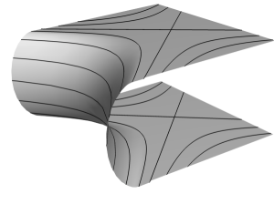
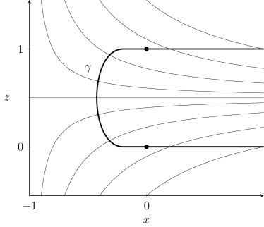
This preserves the planes and generates the standard flow on hyperbolae in -space. For each the lines divide the plane into four invariant quadrants. Let denote the plane with the quadrant containing removed. Now let be a smooth curve in the plane which connects to the origin as shown in Figure 2 [Lee13, Ch. 2], and let denote the set of all orbits of (2) intersecting . Consider the surface
| (3) |
as shown in Figure 1. This surface is smooth and diffeomorphic to the plane, and hence, implicitly defines a linearizing embedding of a planar system with two isolated equilibria as shown in the figure.

Remark 2.
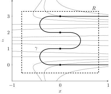
We may extend the previous example to give a planar system with any countable number of isolated equilibria. We do this by continuing to stack higher planes and alternately removing the quadrants containing . The curve must now smoothly snake upwards joining the equilibria together, as shown for instance in Figure 3. We shall denote the surface with exactly equilibria constructed in this way by .
Remark 3.
We may enlarge such systems on the plane to for any by writing and setting, for instance, . The map now defines a linearizing embedding of a system on with any desired countable number of isolated equilibria.
The surface is not given by a graphlike embedding of into . However, it might be possible to find an equivariant embedding of into some higher dimensional vector space whose restriction to is graphlike and hence a super-linearizing embedding of some dynamical system. This is the main idea that we use in our proof of Theorem 1. Before presenting the proof we must first discuss equivariant polynomial maps between vector spaces.
Consider a finite-dimensional vector space . The symmetric product can be interpreted as homogeneous degree- polynomials on the dual by taking the evaluation of on to be the product
Here denotes the pairing between with its dual and is the symmetrized tensor product [FH91, pp. 473–474]. We can then introduce the direct sum
| (4) |
interpreted as the vector space of all degree- polynomials on . The diagonal inclusion given by is a -equivariant degree- polynomial map, and by extension we may consider the natural map
| (5) |
More explicitly, sends to the polynomial which when evaluated on yields
Note that is a smooth embedding of into and is -equivariant with respect to the action on polynomials given by
for and where is the adjoint. Thus, if is a linearizing embedding, so is .
Proposition 1.
Let be a smooth embedding of into a real vector space . The composition is a graphlike embedding if and only if there exist polynomials of degree on for which the fibres of intersect the image of transversely in at most one point.
We will say that the submanifold is tamed by the polynomials .
Proof.
Recall that an embedding is graphlike if and only if there exists a codimension- subspace of whose affine translates intersect the image of the embedding transversely in at most one point. Equivalently, there exist linear functions for which each fibre of intersects the image of the embedding transversely in at most one point. Consequently, is graphlike if and only if there exist in with this property. The result follows by noting that linear functions on pull back through to polynomials of degree on . ∎
Example 2 (A super-linearizing embedding of a planar system with two isolated equilibria).
Consider the planar dynamical system with linearizing embedding from Example 1. Using Proposition 1 we will show that this admits a super-linearizing embedding into the much larger 20-dimensional vector space by finding two degree-3 polynomials and on which tame the surface .
We begin by choosing . Now consider the intersections of with the planes , as shown for instance in Figure 2 for . For any fixed value of , this intersection viewed in the -plane extends in the negative -direction no further than , since is constant along orbits. Therefore, the curve
| (6) |
for any and for fixed, intersects transversely in at most one point. Hence, we set to establish that and tame as intended.
Proof of Theorem 1.
From the previous example we have already established the claim for the case of two isolated equilibria and . By the technique of Remark 3 it suffices to show that the extended surfaces constructed in Remark 2 for finite can also be tamed by some degree polynomials and . By Proposition 1 this will imply that is an equivariant graphlike embedding, and hence, a super-linearizing embedding of some smoothly conjugate dynamical system.
We again set and consider the intersections as shown for instance in Figure 3 for . We claim that for any fixed , the level sets of
| (7) |
transversely intersect the curve , where is any positive constant larger than
and is some closed rectangular region in the plane with and which contains all of the turns of , as shown for instance in Figure 3. To see why this is true consider the gradient of in the plane ,
For different fixed , rectangular regions containing the orbits through the turns of can be chosen to scale in the -direction by a factor less than . Therefore, by construction along the turns of . Furthermore, the sign of always agrees with the sign of the -derivative of . It follows that the derivative of along the curve as it moves upwards is positive everywhere. Each joint level set of and therefore intersects the surface transversely exactly once, as desired. ∎
Remark 4.
It is tempting to extend this proof to include the surface in Example 2 with countably infinite isolated equilibria. However, a direct generalisation will not work. To see why, consider again the intersection . This intersection is now a curve which snakes upwards with infinitely many turns. Suppose this curve can be tamed by some polynomial . Then the derivative of along must be nowhere zero, and hence must alternate sign infinitely often along the line . This contradicts the Fundamental Theorem of Algebra since is a polynomial in .
Incidentally, the example of in the previous remark shows that not every embedded submanifold can be tamed by polynomials. If one is interested in applying a polynomial embedding to super-linearize a dynamical system, it would be of interest to obtain necessary and sufficient conditions for an embedded submanifold to be tamed by polynomials, and to perhaps bound their degree.
To conclude, we would like to make some comments regarding the relevance of these counterexamples to the study of Koopman eigenmappings. For a dynamical system a Koopman eigenfunction is a function on for which
for all and for some . If one has multiple Koopman eigenfunctions then defines an equivariant map from into a linear dynamical system on . If one has enough functionally independent Koopman eigenfunctions, then this map will be a smooth immersion, and hence, is very closely related to our notion of a linearizing embedding. Indeed, in Example 1 the three functions , , and each pull back through the embedding to give Koopman eigenfunctions on a planar dynamical system with multiple isolated equilibria.
As far as we know, these are the first examples of globally defined smooth Koopman eigenfunctions for a dynamical system with multiple isolated equilibria. Furthermore, the linear span of these eigenfunctions seems to be the first known example of a non-trivial finite-dimensional subspace of smooth functions for a dynamical system with multiple isolated equilibria which is invariant under the action of the Koopman operator. Moreover, by using a super-linearizing embedding (as in Example 2) such an invariant subspace additionally “contains the state”.
Finally, we should caution that despite the counterexamples we have presented, there exist many obstructions which prevent the existence of linearizing embeddings for general dynamical systems. The existence of hetero- and homoclinic orbits between equilibria is one such obstruction (since these orbit types are not possible for linear systems), and so too is the presence of multiple asymptotically stable equilibria (see the first footnote in [KA23]). In addition, the main theorem of [LOS23] forbids the existence of linearizing embeddings for systems whose collection of -limit set is countable and contains more than one element, and whose forward-orbits are all precompact. We note that this is consistent with our example since it contains unbounded forward-orbits which are not precompact.
References
- [BBKK22] S L Brunton, M Budišić, E Kaiser, and J N Kutz, Modern Koopman theory for dynamical systems, SIAM Rev. 64 (2022), no. 2, 229–340. MR 4416982
- [BC23] M-A Belabbas and X Chen, A sufficient condition for the super-linearization of polynomial systems, arXiv preprint arXiv:2301.04048 (2023).
- [FH91] W Fulton and J Harris, Representation theory, Graduate Texts in Mathematics, vol. 129, Springer-Verlag, New York, 1991, A first course, Readings in Mathematics. MR 1153249
- [KA23] M D Kvalheim and P Arathoon, Linearizability of flows by embeddings, arXiv preprint arXiv:2305.18288 (2023).
- [Lee13] J M Lee, Introduction to smooth manifolds, second ed., Graduate Texts in Mathematics, vol. 218, Springer, New York, 2013. MR 2954043
- [LOS23] Z Liu, N Ozay, and E D Sontag, On the non-existence of immersions for systems with multiple omega-limit sets, IFAC World Congress, Yokohoma, Japan, to appear (2023), preprint retrieved on May 16, 2023 from webpage at http://ftp.eecs.umich.edu/~necmiye/pubs/LiuOS_ifac23.pdf.