Knowledge Graph Reasoning with Relational Digraph
Abstract.
Reasoning on the knowledge graph (KG) aims to infer new facts from existing ones. Methods based on the relational path have shown strong, interpretable, and transferable reasoning ability. However, paths are naturally limited in capturing local evidence in graphs. In this paper, we introduce a novel relational structure, i.e., relational directed graph (r-digraph), which is composed of overlapped relational paths, to capture the KG’s local evidence. Since the r-digraphs are more complex than paths, how to efficiently construct and effectively learn from them are challenging. Directly encoding the r-digraphs cannot scale well and capturing query-dependent information is hard in r-digraphs. We propose a variant of graph neural network, i.e., RED-GNN, to address the above challenges. Specifically, RED-GNN makes use of dynamic programming to recursively encodes multiple r-digraphs with shared edges, and utilizes query-dependent attention mechanism to select the strongly correlated edges. We demonstrate that RED-GNN is not only efficient but also can achieve significant performance gains in both inductive and transductive reasoning tasks over existing methods. Besides, the learned attention weights in RED-GNN can exhibit interpretable evidence for KG reasoning. 111The code is available at https://github.com/AutoML-Research/RED-GNN/. Correspondence is to Q. Yao.
1. Introduction
Knowledge graph (KG), which contains the interactions among real-world objects, peoples, concepts, etc., brings much connection between artificial intelligence and human knowledge (Battaglia et al., 2018; Ji et al., 2020; Hogan et al., 2021). The interactions are represented as facts with the triple form (subject entity, relation, object entity) to indicate the relation between entities. The real-world KGs are large and highly incomplete (Wang et al., 2017; Ji et al., 2020), thus inferring new facts is challenging. KG reasoning simulates such a process to deduce new facts from existing facts (Chen et al., 2020). It has wide application in semantic search (Berant and Liang, 2014), recommendation (Cao et al., 2019), and question answering (Abujabal et al., 2018), etc. In this paper, we focus on learning the relational structures for reasoning on the queries in the form of (subject entity, relation, ?).
Over the last decade, triple-based models have gained much attention to learn semantic information in KGs (Wang et al., 2017). These models directly reason on triples with the entity and relation embeddings, such as TransE (Bordes et al., 2013), ConvE (Dettmers et al., 2017), ComplEx (Trouillon et al., 2017), RotatE (Sun et al., 2019), QuatE (Zhang et al., 2019a), AutoSF (Zhang et al., 2020b), etc. Since the triples are independently learned, they cannot explicitly capture the local evidence (Niepert, 2016; Xiong et al., 2017; Yang et al., 2017; Teru et al., 2020), i.e., the local structures around the query triples, which can be used as evidence for KG reasoning (Niepert, 2016).
Learning on paths can help to better capture local evidences in graphs since they can preserve sequential connections between nodes (Perozzi et al., 2014; Grover and Leskovec, 2016). Relational path is the first attempt to capture both the semantic and local evidence for reasoning (Lao and Cohen, 2010). DeepPath (Xiong et al., 2017), MINERVA (Das et al., 2017) and M-walk (Shen et al., 2018) use reinforcement learning (RL) to sample relational paths that have strong correlation with the queries. Due to the sparse property of KGs, the RL approaches are hard to train on large-scale KGs (Chen et al., 2020). PathCon (Wang et al., 2021) samples all the relational paths between the entities and use attention mechanism to weight the different paths, but is expensive for the entity query tasks. The rule-based methods, such as RuleN (Meilicke et al., 2018), Neural LP (Yang et al., 2017), DRUM (Sadeghian et al., 2019) and RNNLogic (Qu et al., 2021), generalize the relational paths as logical rules, which learn to infer relations by logical composition of relations, and can provide interpretable insights. Besides, the logical rules can handle inductive reasoning where there exist unseen entities in the inference, which are common in real-world applications (Yang et al., 2017; Sadeghian et al., 2019; Zhang and Chen, 2019).
Subgraphs can naturally be more informative than paths in capturing the local evidence (Battaglia et al., 2018; Ding et al., 2021; Xiao et al., 2021). Their effectiveness has been empirically verified in, e.g., graph-based recommendation (Zhang and Chen, 2019; Zhao et al., 2017) and node representation learning (Hamilton et al., 2017). With the success of graph neural network (GNN) (Gilmer et al., 2017; Kipf and Welling, 2016) in modeling graph-structured data, GNN has been introduced to capture the subgraph structures in KG. R-GCN (Schlichtkrull et al., 2018), CompGCN (Vashishth et al., 2019) and KE-GCN (Yu et al., 2021) propose to update the representations of entities by aggregating all the neighbors in each layer. However, they cannot distinguish the structural role of different neighbors and cannot be interpretable. DPMPN (Xu et al., 2019) learns to reduce the size of subgraph for reasoning on large-scale KGs by pruning the irrelevant entities for a given query rather than learning the specific local structures. p-GAT (Harsha V. et al., 2020) jointly learns a Graph Attention Network and a Markov Logic Network to bridge the gap between embeddings and rules. However, a set of rules must be pre-defined and the expensive EM-algorithm should be used for optimization. Recently, GraIL (Teru et al., 2020) proposes to predict relation from the local enclosing subgraph and shows the inductive ability of subgraph. However, it suffers from both effectiveness and efficiency problems due to the limitation of the enclosing subgraph.
Inspired by the interpretable and transferable abilities of path-based methods and the structure preserving property of subgraphs, we introduce a novel relational structure into KG, called r-digraph, to combine the best of both worlds. The r-digraphs generalize relational paths to subgraphs by preserving the overlapped relational paths and the structures of relations for reasoning. Different from the relational paths that have simple structures, how to efficiently construct and learn from the r-digraphs are challenging since the construction process is expensive (Teru et al., 2020; Wang et al., 2021). Inspired by saving computation costs in overlapping sub-problems using dynamic programming, we propose RED-GNN, a variant of GNN (Gilmer et al., 2017), to recursively encode multiple RElational Digraphs (r-digraphs) with shared edges and select the strongly correlated edges through query-dependent attention weights. Empirically, RED-GNN shows significant gains over the state-of-the-art reasoning methods in both inductive and transductive benchmarks. Besides, the training and inference processes are efficient, the number of model parameters are small, and the learned structures are interpretable.
2. Related Works
A knowledge graph is in the form of , where , and are the sets of entities, relations and fact triples, respectively. Let be the query entity, be query relation, and be answer entity. Given the query , the reasoning task is to predict the missing answer entity . Generally, all the entities in are candidates for (Chen et al., 2020; Das et al., 2017; Yang et al., 2017).
The key for KG reasoning is to capture the local evidence, i.e., entities and relations around the query triples . We regard as missing link, thus the local evidence does not contain this triplet in. Examples of such local evidence explored in the literature are relational paths (Das et al., 2017; Lao et al., 2011; Xiong et al., 2017; Wang et al., 2021) and subgraphs (Schlichtkrull et al., 2018; Teru et al., 2020; Vashishth et al., 2019). In this part, we introduce the path-based methods and GNN-based methods that leverage structures in for reasoning.
2.1. Path-based methods
Relational path (Definition 1) is a set of triples that are sequentially connected. The path-based methods learn to predict the triple by a set of relational paths as local evidence. DeepPath (Xiong et al., 2017) learns to generate the relational path from to by reinforcement learning (RL). To improve the efficiency, MINERVA (Das et al., 2017) and M-walk (Shen et al., 2018) learn to generate multiple paths starting from by RL. The scores are indicated by the arrival frequency on different ’s. Due to the complex structure of KG, the reward is very sparse, making it hard to train the RL models (Chen et al., 2020). PathCon (Wang et al., 2021) samples all the paths connecting the two entities to predict the relation between them, which is expensive for the reasoning task .
Definition 0 (Relational path (Lao et al., 2011; Xiong et al., 2017; Zhang et al., 2020a)).
The relational path with length is a set of triples , , , , that are connected head-to-tail sequentially.
Instead of directly using paths, the rule-based methods learn logical rules as a generalized form of relational paths. The logical rules are formed with the composition of a set of relations to infer a specific relation. This can provide better interpretation and can be transfered to unseen entities. The rules are learned by either the mining methods like RuleN (Meilicke et al., 2018), EM algorithm like RNNLogic (Qu et al., 2021), or end-to-end training, such as Neural LP (Yang et al., 2017) and DRUM (Sadeghian et al., 2019), to generate highly correlated relational paths between and . The rules can provide logical interpretation and transfer to unseen entities. However, the rules only capture the sequential evidences, thus cannot learn more complex patterns such as the subgraph structures.
2.2. GNN-based methods
As mentioned in Section 1, the subgraphs can preserve richer information than the relational paths as more degree are allowed in the subgraph. GNN has shown strong power in modeling the graph structured data (Battaglia et al., 2018). This inspires recent works, such as R-GCN (Schlichtkrull et al., 2018), CompGCN (Vashishth et al., 2019), and KE-GCN (Yu et al., 2021), extending GNN on KG to aggregate the entities’ and relations’ representations under the message passing framework (Gilmer et al., 2017) as
| (1) |
which aggregates the message on the -hop neighbor edges of entity with dimension . is a weighting matrix, is the activation function and is the relation representation in the -th layer. After layers’ aggregation, the representations capturing the local structures of entities jointly work with a decoder scoring function to measure the triples. Since the message passing function (1) aggregates information of all the neighbors and is independent with the query, R-GCN and CompGCN cannot capture the explicit local evidence for specific queries and are not interpretable.
Instead of using all the neighborhoods, DPMPN (Xu et al., 2019) designs one GNN to aggregate the embeddings of entities, and another GNN to dynamically expand and prune the inference subgraph from the query entity . A query-dependent attention is applied over the sampled entities for pruning. This approach shows interpretable reasoning process by the attention flow on the pruned subgraph, but still requires embeddings to guide the pruning, thus cannot be generalized to unseen entities. Besides, it cannot capture the explicit local evidence supporting a given query triple.
p-GAT (Harsha V. et al., 2020) and pLogicNet (Qu and Tang, 2019) jointly learns an embedding-based model and a Markov logic network (MLN) by variational-EM algorithm. The embedding model generates evidence for MLN to update and MLN expends the training data for embedding model to train. MLN brings the gap between embedding models and logic rules, but it requires a pre-defined set of rules for initialization and the training is expensive with the variational-EM algorithm.
Recently, GraIL (Teru et al., 2020) proposes to extract the enclosing subgraph between the query entity and answer entity . To learn the enclosing subgraph, the relational GNN (Schlichtkrull et al., 2018) with query-dependent attention is applied over the edges in to control the importance of edges for different queries, but the learned attention weights are not interpretable (see Appendix B). After layers’ aggregation, the graph-level representations aggregate all the entities in the subgraph and are used to score the triple . Since the subgraphs need to be explicitly extracted and scored for different triples, the computation cost is very high.
3. Relational Digraph (r-digraph)
The relational paths have shown strong transferable and interpretable reasoning ability on KGs (Das et al., 2017; Yang et al., 2017; Sadeghian et al., 2019). However, they are limited in capturing more complex dependencies in KG since the nodes in paths are only sequentially connected. GNN-based methods can learn different subgraph structures. But none of the existing methods can efficiently learn the subgraph structures that are both interpretable and inductive like rules. Hence, we are motivated to define a new kind of structure, to explore the important local evidence.
Before defining r-digraph, we first introduce a special type of directed graph in Definition 1.
Definition 0 (Layered st-graph (Battista et al., 1998)).
The layered st-graph is a directed graph with exactly one source node (s) and one sink node (t). All the edges are directed, connecting nodes between consecutive layers and pointing from -th layer to -th layer.
Here, we adopt the general approaches to augment the triples with reverse and identity relations (Vashishth et al., 2019; Sadeghian et al., 2019). Then, all the relational paths with length less than or equal to between and can be represented as relational paths with length . In this way, they can be formed as paths in a layered st-graph, with the single source entity and sink entity . Such a structure preserves all the relational paths between and up to length , and maintains the subgraph structures. Based on this observation, we define r-digraph in Definition 2.
Definition 0 (r-digraph).
The r-digraph is a layered st-graph with the source entity and the sink entity . The entities in the same layer are different with each other. Any path pointing from to in the r-digraph is a relational path with length , where connects an entity in the -layer to an entity in -layer. We define if there is no relational path connecting and with length .
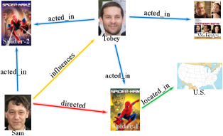
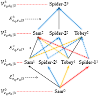
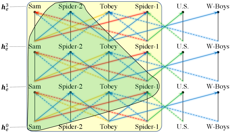
Figure 1(b) provides an example of r-digraph , which is used to infer the new triple (Sam, directed, Spider-2), in the exemplar KG in Figure 1(a). Inspired by the reasoning ability of relational paths (Das et al., 2017; Yang et al., 2017; Sadeghian et al., 2019), we aim to leverage the r-digraph for KG reasoning. However, different from the relational paths which have simple structures to learn with sequential models (Xiong et al., 2017; Das et al., 2017), how to efficiently construct and how to effectively learn from the r-digraphs are challenging.
In the paper, are the edges and are the entities in the -th layer of the r-digraph
with denoting the layer-wise connection. We define the union operator as . Given an entity , we denote , and as the sets of out-edges, in-edges and entities, respectively, visible in steps walking from . and are graphically shown in Figure 1.
4. The Proposed Model
Here, we show how GNNs can be tailor-made to efficiently and effectively learn from the r-digraphs. Extracting subgraph structures and then learning the subgraph representation is a common practice for subgraph encoding in the literature, such as GraphSage (Hamilton et al., 2017) and GraIL (Teru et al., 2020). Given a query triple , the subgraph encoding generally contains three processes:
-
(i).
extract the neighborhoods of both and ;
-
(ii).
take the intersection to construct the subgraph;
-
(iii).
run message passing and use the graph-level representation as the subgraph encoding.
When working on the r-digraph , the same approach can be customized in Algorithm 1. First, we get the neighborhoods of both and in steps 2-5. Second, we take the intersection of neighborhoods from and in steps 6-8 to induce the r-digraph layer-wisely. Third, if the r-digraph is empty, we set the representation as in step 9. Otherwise, the message passing is conducted layer-by-layer in steps 10-12. Since is the single sink entity, the final layer representation is used as subgraph representation to encode the r-digraph . We name this simple solution as RED-Simp.
However, Algorithm 1 is very expensive. First, we need to conduct the two directional sampling in steps 3 and 4, and take the intersection to extract the r-digraph. Second, given a query , we need to do this algorithm for different triples with different answering entities . It needs time (see Section 4.3) to predict a given query , where is the average degree of entities in and is the average number of edges in ’s. These limitations also exist in PathCon (Wang et al., 2021) and GraIL (Teru et al., 2020). To improve efficiency, we propose to encode multiple r-digraphs recursively in Section 4.1.
4.1. Recursive r-digraph encoding
In Algorithm 1, when evaluating with different but the same query , the neighboring edges of are shared. We have the following observation:
Proposition 1.
The set of edges visible from by -steps equals , namely is the union of the -th layer edges in the r-digraphs between and all the entities .
Proposition 1 indicates that the -th layer edges with different answer entities share the same set of edges in . A common approach to save computation cost in overlapping sub-problems is dynamic programming. This has been used to aggregate node representations on large-scale graphs (Hamilton et al., 2017) or to propagate the question representation on KGs (Zhang et al., 2018). Inspired by the efficiency gained by dynamic programming, we recursively construct the r-digraph between and any entity as
| (2) |
Once the representations of for all the entities in the -th layer are ready, we can encode by combining with the shared edges in the -th layer. Based on Proposition 1 and Eq.(2), we are motivated to recursively encode multiple r-digraphs with the shared edges in layer by layer. The full process is in Algorithm 2.
Initially, only is visible in . In the -th layer, we collect the edges and entities in step 3. Then, the message passing is constrained to obtain the representations for through the edges in . Finally, the representations , encoding for all the entities , are returned in step 7. The recursive encoding can be more efficient with shared edges in and fewer loops. It learns the same representations as Algorithm 1 as guaranteed by Proposition 2.
4.2. Interpretable reasoning with r-digraph
As the construction of is independent with the query relation , how to encode is another problem to address. Given different triples sharing the same r-digraph, e.g. (Sam, starred, Spider-2) and (Sam, directed, Spider-2), the local evidence we use for reasoning is different. To capture the query-dependent knowledge from the r-digraphs and discover interpretable local evidence, we use the attention mechanism (Veličković et al., 2017) and encode into the attention weight to control the importance of different edges in . The message passing function is specified as
| (3) |
where the attention weight on edge is
| (4) |
with , , and is the concatenation operator. Sigmoid function is used rather than softmax attention (Veličković et al., 2017) to ensure multiple edges can be selected in the same neighborhood.
After layers’ aggregation by (3), the representations can encode essential information for scoring . Hence, we design a simple scoring function
| (5) |
with . We associate the multi-class log-loss (Lacroix et al., 2018) with each training triple , i.e.,
| (6) |
The first part in (6) is the score of the positive triple in , the set of training queries, and the second part contains the scores of all triples with the same query . The model parameters , , , , are randomly initialized and are optimized by minimizing (6) with stochastic gradient descent (Kingma and Ba, 2014).
We provide Theorem 1 to show that if a set of relational paths are strongly correlated with the query triple, they can be identified by the attention weights in RED-GNN, thus being interpretable. This theorem is also empirically illustrated in Section 5.4.
Theorem 1.
Given a triple , let be a set of relational paths , that are generated by a set of rules between and with the form
where are variables that are bounded by unique entities. Denote as the r-digraph constructed by . There exists a parameter setting and a threshold for RED-GNN that can equals to the r-digraph, whose edges have attention weights , in .
4.3. Inference complexity
In this part, we compare the inference complexity of different GNN-based methods. When reasoning on the query , we need to evaluate triples with the different answer entity . We assume the average degree as and average number of edges in each layer of r-digraph as .
-
•
RED-Simp (Algorithm 1). For construction, the main cost, which is with the worst case cost , comes from extracting the neighborhoods of and . Along with encoding, the total cost is .
-
•
RED-GNN (Algorithm 2). Since the full computation is conducted on and , thus the cost is the number of edges times the dimension , i.e. and .
-
•
CompGCN. All the representations are aggregated in one pass with cost . Then the scores for all the entities are computed with cost . The total cost is .
-
•
DPMPN. Denote the dimension and layer in the non-attentive GNN as , the average sampled edges in the pruning procedure as . The main cost comes from the non-attentive GNN with cost . The cost on sampled subgraph is . Thus, the total computation cost is .
-
•
GraIL. Denote as the average number of entities in the subgraphs. The complexity in constructing the enclosing subgraph is with edges and entities. The cost of the GNN module is . Then the overall cost is .
In comparison, we have RED-GNN CompGCN DPMPN RED-Simp GraIL in terms of inference complexity. The empirical evaluation is provided in Section 5.3.
5. Experiments
All the experiments are written in Python with PyTorch framework (Paszke et al., 2017) and run on an RTX 2080Ti GPU with 11GB memory.
5.1. Inductive reasoning
Inductive reasoning is a hot research topic (Hamilton et al., 2017; Sadeghian et al., 2019; Teru et al., 2020; Yang et al., 2017) as there are emerging new entities in the real-world applications, such as new users, new items and new concepts (Zhang and Chen, 2019). Being able to reason on unseen entities requires the model to capture the semantic and local evidence ignoring the identity of entities.
| WN18RR | FB15k-237 | NELL-995 | |||||||||||
| V1 | V2 | V3 | V4 | V1 | V2 | V3 | V4 | V1 | V2 | V3 | V4 | ||
| MRR | RuleN | .668 | .645 | .368 | .624 | .363 | .433 | .439 | .429 | .615 | .385 | .381 | .333 |
| Neural LP | .649 | .635 | .361 | .628 | .325 | .389 | .400 | .396 | .610 | .361 | .367 | .261 | |
| DRUM | .666 | .646 | .380 | .627 | .333 | .395 | .402 | .410 | .628 | .365 | .375 | .273 | |
| GraIL | .627 | .625 | .323 | .553 | .279 | .276 | .251 | .227 | .481 | .297 | .322 | .262 | |
| RED-GNN | .701 | .690 | .427 | .651 | .369 | .469 | .445 | .442 | .637 | .419 | .436 | .363 | |
| Hit@1 (%) | RuleN | 63.5 | 61.1 | 34.7 | 59.2 | 30.9 | 34.7 | 34.5 | 33.8 | 54.5 | 30.4 | 30.3 | 24.8 |
| Neural LP | 59.2 | 57.5 | 30.4 | 58.3 | 24.3 | 28.6 | 30.9 | 28.9 | 50.0 | 24.9 | 26.7 | 13.7 | |
| DRUM | 61.3 | 59.5 | 33.0 | 58.6 | 24.7 | 28.4 | 30.8 | 30.9 | 50.0 | 27.1 | 26.2 | 16.3 | |
| GraIL | 55.4 | 54.2 | 27.8 | 44.3 | 20.5 | 20.2 | 16.5 | 14.3 | 42.5 | 19.9 | 22.4 | 15.3 | |
| RED-GNN | 65.3 | 63.3 | 36.8 | 60.6 | 30.2 | 38.1 | 35.1 | 34.0 | 52.5 | 31.9 | 34.5 | 25.9 | |
| Hit@10 (%) | RuleN | 73.0 | 69.4 | 40.7 | 68.1 | 44.6 | 59.9 | 60.0 | 60.5 | 76.0 | 51.4 | 53.1 | 48.4 |
| Neural LP | 77.2 | 74.9 | 47.6 | 70.6 | 46.8 | 58.6 | 57.1 | 59.3 | 87.1 | 56.4 | 57.6 | 53.9 | |
| DRUM | 77.7 | 74.7 | 47.7 | 70.2 | 47.4 | 59.5 | 57.1 | 59.3 | 87.3 | 54.0 | 57.7 | 53.1 | |
| GraIL | 76.0 | 77.6 | 40.9 | 68.7 | 42.9 | 42.4 | 42.4 | 38.9 | 56.5 | 49.6 | 51.8 | 50.6 | |
| RED-GNN | 79.9 | 78.0 | 52.4 | 72.1 | 48.3 | 62.9 | 60.3 | 62.1 | 86.6 | 60.1 | 59.4 | 55.6 | |
| type | models | Family | UMLS | WN18RR | FB15k-237 | NELL-995 | ||||||||||
|---|---|---|---|---|---|---|---|---|---|---|---|---|---|---|---|---|
| MRR | Hit@1 | Hit@10 | MRR | Hit@1 | Hit@10 | MRR | Hit@1 | Hit@10 | MRR | Hit@1 | Hit@10 | MRR | Hit@1 | Hit@10 | ||
| triple | ConvE* | - | - | - | .94 | 92. | 96. | .43 | 39. | 49. | .325 | 23.7 | 50.1 | - | - | - |
| RotatE | .921 | 86.6 | 98.8 | .925 | 86.3 | 99.3 | .477 | 42.8 | 57.1 | .337 | 24.1 | 53.3 | .508 | 44.8 | 60.8 | |
| QuatE | .941 | 89.6 | 99.1 | .944 | 90.5 | 99.3 | .480 | 44.0 | 55.1 | .350 | 25.6 | 53.8 | .533 | 46.6 | 64.3 | |
| path | MINERVA | .885 | 82.5 | 96.1 | .825 | 72.8 | 96.8 | .448 | 41.3 | 51.3 | .293 | 21.7 | 45.6 | .513 | 41.3 | 63.7 |
| Neural LP | .924 | 87.1 | 99.4 | .745 | 62.7 | 91.8 | .435 | 37.1 | 56.6 | .252 | 18.9 | 37.5 | out of memory | |||
| DRUM | .934 | 88.1 | 99.6 | .813 | 67.4 | 97.6 | .486 | 42.5 | 58.6 | .343 | 25.5 | 51.6 | out of memory | |||
| RNNLogic* | – | – | – | .842 | 77.2 | 96.5 | .483 | 44.6 | 55.8 | .344 | 25.2 | 53.0 | – | – | – | |
| GNN | pLogicNet* | – | – | – | .842 | 77.2 | 96.5 | .441 | 39.8 | 53.7 | .332 | 23.7 | 52.8 | – | – | – |
| CompGCN | .933 | 88.3 | 99.1 | .927 | 86.7 | 99.4 | .479 | 44.3 | 54.6 | .355 | 26.4 | 53.5 | out of memory | |||
| DPMPN | .981 | 97.4 | 98.1 | .930 | 89.9 | 98.2 | .482 | 44.4 | 55.8 | .369 | 28.6 | 53.0 | .513 | 45.2 | 61.5 | |
| RED-GNN | .992 | 98.8 | 99.7 | .964 | 94.6 | 99.0 | .533 | 48.5 | 62.4 | .374 | 28.3 | 55.8 | .543 | 47.6 | 65.1 | |
Setup. We follow the general inductive setting (Sadeghian et al., 2019; Teru et al., 2020; Yang et al., 2017) where there are new entities in testing and the relations are the same as those in training. Specifically, the training and testing contain two KGs and , with the same set of relations but disjoint sets of entities. Three sets of triples , augmented with reverse relations, are provided. is used to predict and for training and validation, respectively. In testing, is used to predict . Same as (Sadeghian et al., 2019; Teru et al., 2020; Yang et al., 2017), we use the filtered ranking metrics, i.e., mean reciprocal rank (MRR), Hit@1 and Hit@10 (Bordes et al., 2013), to indicate better performance with larger values.
Baselines. Since training and testing contain disjoint sets of entities, all the methods requiring the entity embeddings (Bordes et al., 2013; Harsha V. et al., 2020; Sun et al., 2019; Vashishth et al., 2019; Xu et al., 2019; Zhang et al., 2019a) cannot be applied here. We mainly compare with four methods: 1) RuleN (Meilicke et al., 2018), the discrete rule induction method; 2) Neural-LP (Yang et al., 2017), the first differentiable method for rule learning; 3) DRUM (Sadeghian et al., 2019), an improved work of Neural-LP (Yang et al., 2017); and 4) GraIL (Teru et al., 2020), which designs the enclosing subgraph for inductive reasoning. MINERVA (Das et al., 2017), PathCon (Wang et al., 2021) and RNNLogic (Qu et al., 2021) can potentially work on this setting but there lacks the customized source code for the inductive setting, thus not compared.
Hyper-parameters. For RED-GNN, we tune the learning rate in , weight decay in , dropout rate in , batch size in , dimension in , for attention in , layer in , and activation function in {identity, tanh, ReLU}. Adam (Kingma and Ba, 2014) is used as the optimizer. The best hyper-parameter settings are selected by the MRR metric on with maximum training epochs of 50. For RuleN, we use their implementation with default setting. For Neural LP and DRUM, we tune the learning rate in , dropout rate in , batch size in , dimension in , layer of RNN in , and number of steps in . For GraIL we tune the learning rate in , weight decay in , batch size in , dropout rate in , edge_dropout rate in , GNN aggregator among {sum, MLP, GRU} and hop numbers among . The training epochs are all set as 50.
Tie policy. In evaluation, the tie policy is important. Specifically, when there are triples with the same rank, choosing the largest rank and smallest rank in a tie will lead to rather different results (Sun et al., 2020). Considering that we give the same score for triples where , there will be a concern of the tie policy. Hence, we use the average rank among the triples in tie as suggested (Rossi et al., 2021).
Datasets. We use the benchmark dataset in (Teru et al., 2020), created on WN18RR (Dettmers et al., 2017), FB15k237 (Toutanova and Chen, 2015) and NELL-995 (Xiong et al., 2017). Each dataset includes four versions with different groups of triples. Please refer to (Teru et al., 2020) for more details.
Results. The performance is shown in Table 1. First, GraIL is the worst among all the methods since the enclosing subgraphs do not learn well of the relational structures that can be generalized to unseen entities (more details in Appendix B). Second, there is not absolute winner among the rule-based methods as different rules adapt differently to these datasets. In comparison, RED-GNN outperforms the baselines across all the benchmarks. Based on Thereom 1, the attention weights can help to adaptively learn correlated relational paths for different datasets, and preserve the structural patterns at the same time. In some cases, the Hit@10 of RED-GNN is slightly worse than the rule-based methods since it may overfit to the top-ranked samples.
5.2. Transductive reasoning
Transductive reasoning, also known as KG completion (Trouillon et al., 2017; Wang et al., 2017), is another general setting in the literature. It evaluates the models’ ability to learn the patterns on an incomplete KG.
Setup. In this setting, a KG and the query triples , augmented with reverse relations, are given. For the triple-based method, triples in are used for training, and are used for inference. For the others, of the triples in are used to extract paths/subgraphs to predict the remaining triples in training, and the full set is then used to predict in inference (Yang et al., 2017; Sadeghian et al., 2019). We use the same filtered ranking metrics with the same tie policy in Section 5.1, namely MRR, Hit@1 and Hit@10.
Baselines. We compare RED-GNN with the triple-based methods ConvE (Dettmers et al., 2017), RotatE (Sun et al., 2019) and QuatE (Zhang et al., 2019a); the path-based methods MINERVA (Das et al., 2017), Neural LP (Yang et al., 2017), DRUM (Sadeghian et al., 2019) and RNNLogic (Qu et al., 2021); MLN-based method pLogicNet (Qu and Tang, 2019) and the GNN-based methods CompGCN (Vashishth et al., 2019) and DPMPN (Xu et al., 2019). RuleN (Meilicke et al., 2018) is not compared here since it has been shown to be worse than DRUM (Sadeghian et al., 2019) and RNNLogic (Qu et al., 2021) in this setting. p-GAT is not compared as their results are evaluated on a problematic framework (Sun et al., 2020). GraIL (Teru et al., 2020) is not compared since it is computationally intractable on large graphs (see Section 5.3).
Hyper-parameters. The tuning ranges of hyper-parameters of RED-GNN are the same as those in the inductive reasoning. For RotatE and QuatE, we tune the dimensions in , batch size in , weight decay in , number of negative samples in , with training iterations of 100000. For MINERVA, Neural LP, DRUM and DPMPN, we use their default setting provided. For CompGCN, we choose the decoder as ConvE, the operator as circular correlation as suggested (Vashishth et al., 2019), and tune the learning rate in , layer in and dropout rate in with training epochs of 300.
Datasets. Five 222 Data from https://github.com/alisadeghian/DRUM/tree/master/datasets and https://github.com/thunlp/OpenKE/tree/OpenKE-PyTorch/benchmarks/NELL-995. datasets are used including Family (Kok and Domingos, 2007), UMLS (Kok and Domingos, 2007), WN18RR (Dettmers et al., 2017), FB15k237 (Toutanova and Chen, 2015) and NELL-995 (Xiong et al., 2017). We provide the statistics of entities, relations and split of triples in Table 3.
| Family | 3,007 | 12 | 23,483 | 2,038 | 2,835 |
|---|---|---|---|---|---|
| UMLS | 135 | 46 | 5,327 | 569 | 633 |
| WN18RR | 40,943 | 11 | 86,835 | 3,034 | 3,134 |
| FB15k-237 | 14,541 | 237 | 272,115 | 17,535 | 20,466 |
| NELL-995* | 74,536 | 200 | 149,678 | 543 | 2,818 |
Results. As in Table 2, the triple-based methods are better than the path-based ones on Family and UMLS, and is comparable with DRUM and RNNLogic on WN18RR, FB15k-237. The entity embeddings can implicitly preserve local information around entities, while the path-based methods may loss the structural patterns. CompGCN performs similar as the triple-based methods since it mainly relies on the aggregated embeddings and the decoder scoring function. Neural LP, DRUM and CompGCN run out of memory on NELL-995 with entities due to the use of full adjacency matrix. For DPMPN, the entities in the pruned subgraph is more informative than that in CompGCN, thus has better performance. For RED-GNN, it is better than all the baselines indicated by the MRR metric. These demonstrate that the r-digraph can not only transfer well to unseen entities, but also capture the important patterns in incomplete KGs without using entity embeddings.
5.3. Complexity analysis
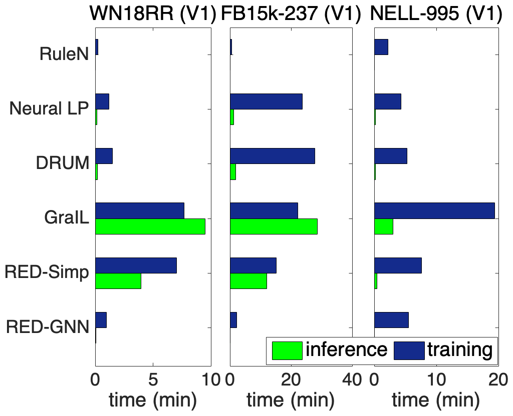
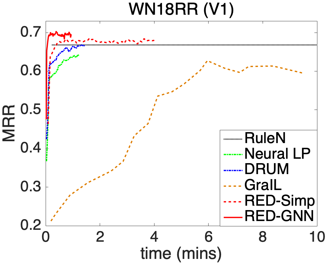
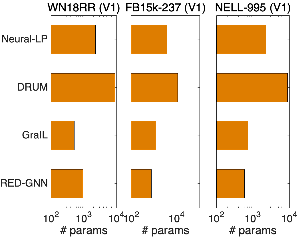
We compare the complexity in terms of running time and parameter size of different methods in this part. We show the training time and the inference time on for each method in Figure 2(a), learning curves in Figure 2(b), and model parameters in Figure 2(c).
Inductive reasoning. We compare RuleN, Neural LP, DRUM, GraIL and RED-GNN on WN18RR (V1), FB15k-237 (V1) and NELL-995 (V1). Both training and inference are very efficient in RuleN. Neural LP and DRUM have similar cost but are more expensive than RED-GNN by using the full adjacency matrix. For GraIL, both training and inference are very expensive since they require bidirectional sampling to extract the subgraph and then compute for each triple. As for model parameters, RED-GNN and GraIL have similar amount of parameters, less than Neural-LP and DRUM. Overall, RED-GNN is more efficient than the differentiable methods Neural LP, DRUM and GraIL.
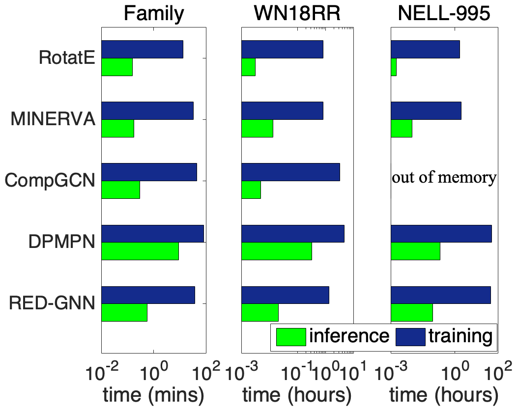
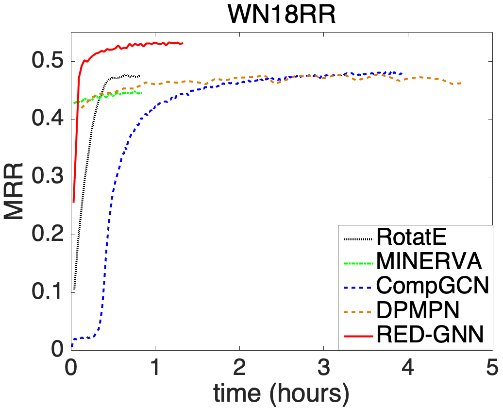
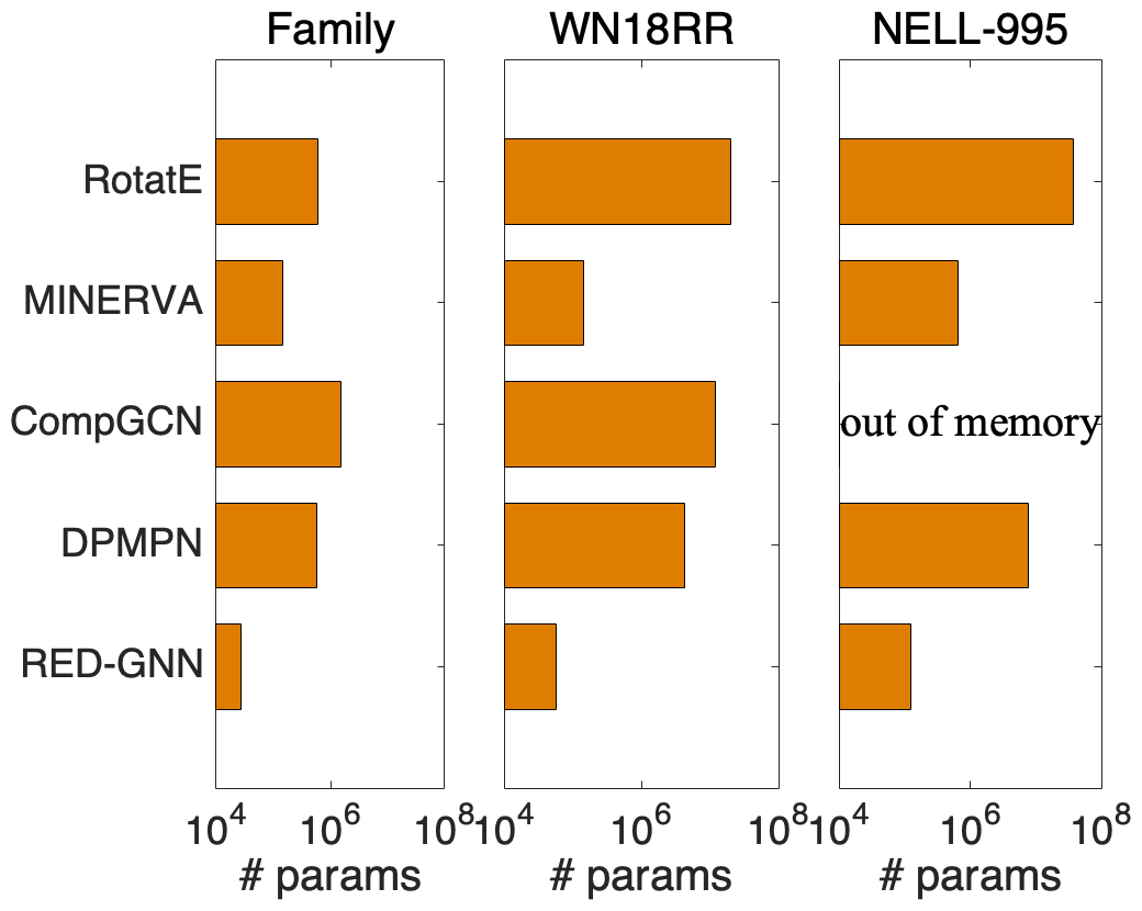
Transductive reasoning. We compare RotatE, MINERVA, CompGCN, DPMPN and RED-GNN on Family, WN18RR and NELL-995. Due to the simple training framework on triples, RotatE is the fastest method. MINERVA is more efficient than GNN-based methods since the sampled paths can be efficiently modeled in sequence. CompGCN, with fewer layers, has similar cost with RED-GNN as its computation is on the whole graph. For DPMPN, the pruning is expensive and it has two GNNs working together, thus it is more expensive than RED-GNN. GraIL is hundreds of times more expensive than RED-GNN, thus intractable on the larger KGs in this setting. Since RED-GNN does not learn entity embeddings, it has much less parameters compared with the other four methods.
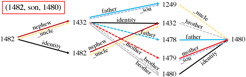
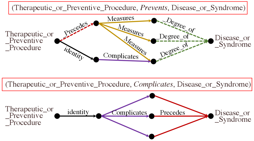
5.4. Case study: learned r-digraphs
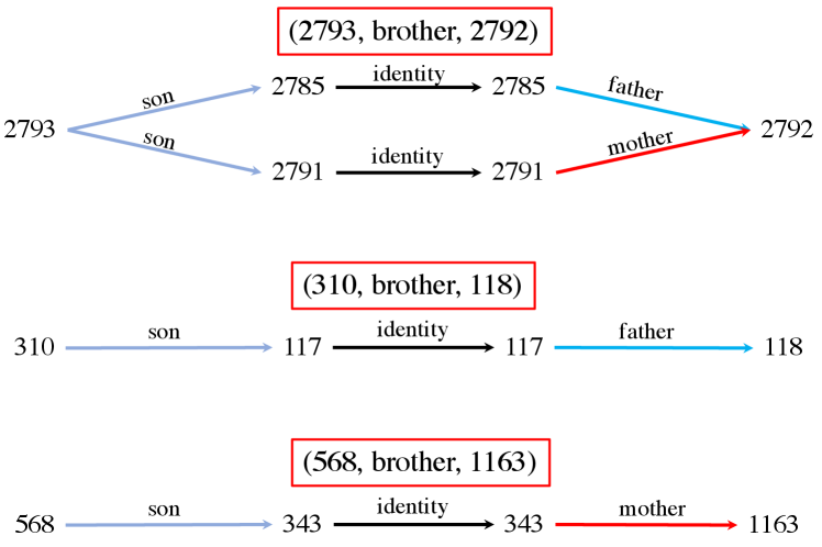
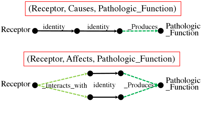
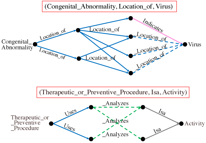
We visualize some exemplar learned r-digraphs by RED-GNN with on the Family and UMLS datasets. Given the triple , we remove the edges in whose attention weights are less than , and extract the remaining parts. Figure 3(a) shows one triple that DRUM fails. As shown, inferring id- as the son of id- requires the knowledge that id- is the only brother of the uncle id- from the local structure. Figure 3(b) shows the example with the same and sharing the same digraph . As shown, RED-GNN can learn distinctive structures for different query relations, which caters to Theorem 1. The examples in Figure 3 demonstrate that RED-GNN is interpretable. We provide more examples and the visualization algorithm in Appendix A.
5.5. Ablation study
Variants of RED-GNN. Table 4 shows the performance of different variants. First, we study the impact of removing in attention (denoted as Attn-w.o.-). Specifically, we remove from the attention weight in (4) and change the scoring function to , with . Since the attention aims to figure out the important edges in , the learned structure will be less informative without the control of the query relation , thus has poor performance.
| WN18RR (V1) | FB15k-237 (V1) | NELL (V1) | ||||
|---|---|---|---|---|---|---|
| methods | MRR | H@10 | MRR | H@10 | MRR | H@10 |
| Attn-w.o.- | .659 | 78.3 | .268 | 37.6 | .517 | 73.4 |
| RED-Simp | .683 | 79.6 | .311 | 45.3 | .563 | 75.8 |
| RED-GNN | .701 | 79.9 | .369 | 48.3 | .637 | 86.6 |
Second, we replace Algorithm 2 in RED-GNN with the simple solution in Algorithm 1, i.e. RED-Simp. Due to the efficiency issue, the loss function (6), which requires to compute the scores over many negative triples, cannot be used. Hence, we use the margin ranking loss with one negative sample as in GraIL (Teru et al., 2020). As in Table 4, the performance of RED-Simp is weak than RED-GNN since the multi-class log loss is better than loss functions with negative sampling (Lacroix et al., 2018; Ruffinelli et al., 2020; Zhang et al., 2019b). RED-Simp still outperforms GraIL in Table 1 since the r-digraphs are better structures for reasoning. The running time of RED-Simp is in Figure 2(a) and 2(b). Algorithm 1 is much more expensive than Algorithm 2 but is cheaper than GraIL since GraIL needs the Dijkstra algorithm to label the entities.
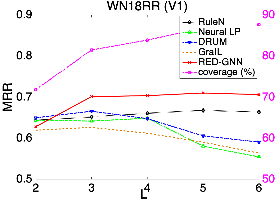
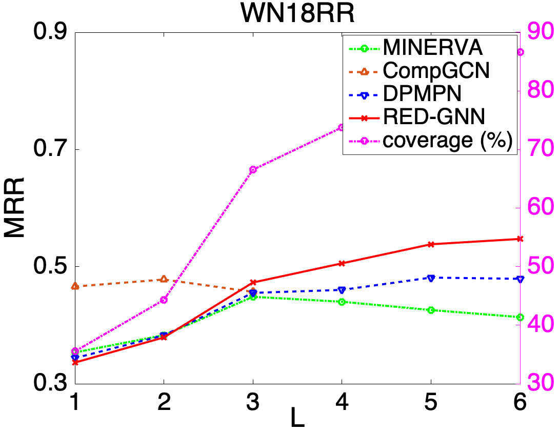
Depth of models. In Figure 4, we show the influence of testing MRR with different layers or steps in the left -axis. The coverage (in %) of testing triples where is visible from in steps, i.e., , is shown in the right -axis. Intuitively, when increases, more triples will be covered, paths or subgraphs between and then contain richer information, but will be harder to learn. As shown, the performance of DRUM, Neural LP and MINERVA decreases for . CompGCN runs out of memory when and it is also hard to capture complex structures with . When is too small, e.g., , RED-GNN has poor performance mainly dues to limited information encoded in such small r-digraphs. RED-GNN achieves the best performance for where the r-digraphs can contain richer information and the important information for reasoning can be effectively learned by (3). Since the computation cost significantly increases with , we tune to balance the efficiency and effectiveness in practice.
| distance | 1 | 2 | 3 | 4 | 5 | 5 |
|---|---|---|---|---|---|---|
| ratios (%) | 34.9 | 9.3 | 21.5 | 7.5 | 8.9 | 17.9 |
| CompGCN | .993 | .327 | .337 | .062 | .061 | .016 |
| DPMPN | .982 | .381 | .333 | .102 | .057 | .001 |
| RED-GNN | .993 | .563 | .536 | .186 | .089 | .005 |
Per-distance performance. Note that given a r-digraph with layers, the information between two nodes that are not reachable with hops cannot be propagated by Algorithm 2. This may raise a concern about the predicting ability of RED-GNN, especially for triples not reachable in steps. We demonstrate this is not a problem here. Specifically, given a triple , we compute the shortest distance from to . Then, the MRR performance is grouped in different distances. We compare CompGCN (), DPMPN () and RED-GNN () in Table 5. All the models have worse performance on triples with larger distance and cannot well model the triples that are far away. RED-GNN has the best per-distance performance within distance .
6. Conclusion
In this paper, we introduce a novel relational structure, i.e., r-digraph, as a generalized structure of relational paths for KG reasoning. Individually computing on each r-digraph is expensive for the reasoning task . Hence, inspired by solving overlapping sub-problems by dynamic programming, we propose RED-GNN as a variant of GNN, to efficiently construct and effectively learn the r-digraph. We show that RED-GNN achieves the state-of-the-art performance in both KG with inductive and transductive KG reasoning benchmarks. The training and inference of RED-GNN are very efficient compared with the other GNN-based baselines. Besides, interpretable structures for reasoning can be learned by RED-GNN.
Lastly, a concurrent work NBFNet (Zhu et al., 2021) proposes to recursively encode all the paths between the query entity to multiple answer entities, which is similar to RED-GNN. However, NBFNet uses the full adjacency matrix for propagation, which is very expensive and requires 128GB GPU memory. In the future work, we can leverage the pruning technique in (Xu et al., 2019) or distributed programming in (Cohen et al., 2019) to apply RED-GNN on KG with extremely large scale.
References
- (1)
- Abujabal et al. (2018) A. Abujabal, R. Saha Roy, M. Yahya, and G. Weikum. 2018. Never-ending learning for open-domain question answering over knowledge bases. In The WebConf. 1053–1062.
- Battaglia et al. (2018) P. Battaglia, J. B Hamrick, V. Bapst, A. Sanchez-Gonzalez, V. Zambaldi, M. Malinowski, et al. 2018. Relational inductive biases, deep learning, and graph networks. Technical Report. arXiv:1806.01261.
- Battista et al. (1998) G. D. Battista, P. Eades, R. Tamassia, and I. G Tollis. 1998. Graph drawing: algorithms for the visualization of graphs. Prentice Hall PTR.
- Berant and Liang (2014) J. Berant and P. Liang. 2014. Semantic parsing via paraphrasing. In ACL. 1415–1425.
- Bordes et al. (2013) A. Bordes, N. Usunier, A. Garcia-Duran, J. Weston, and O. Yakhnenko. 2013. Translating embeddings for modeling multi-relational data. In NeurIPS. 2787–2795.
- Cao et al. (2019) Y. Cao, X. Wang, X. He, Z. Hu, and T. Chua. 2019. Unifying knowledge graph learning and recommendation: Towards a better understanding of user preferences. In The WebConf. 151–161.
- Chen et al. (2020) X. Chen, S. Jia, and Y. Xiang. 2020. A review: Knowledge reasoning over knowledge graph. Expert Systems with Applications 141 (2020), 112948.
- Cohen et al. (2019) W. W Cohen, H. Sun, R A. Hofer, and M. Siegler. 2019. Scalable Neural Methods for Reasoning With a Symbolic Knowledge Base. In ICLR.
- Das et al. (2017) R. Das, S. Dhuliawala, M. Zaheer, L. Vilnis, I. Durugkar, A. Krishnamurthy, A. Smola, and A. McCallum. 2017. Go for a walk and arrive at the answer: Reasoning over paths in knowledge bases using reinforcement learning. In ICLR.
- Dettmers et al. (2017) T. Dettmers, P. Minervini, P. Stenetorp, and S. Riedel. 2017. Convolutional 2D knowledge graph embeddings. In AAAI.
- Ding et al. (2021) Y. Ding, Q. Yao, H. Zhao, and T. Zhang. 2021. Diffmg: Differentiable meta graph search for heterogeneous graph neural networks. In SIGKDD. 279–288.
- Gilmer et al. (2017) J. Gilmer, S. S Schoenholz, P. F Riley, O. Vinyals, and G. E Dahl. 2017. Neural Message Passing for Quantum Chemistry. In ICML. 1263–1272.
- Grover and Leskovec (2016) A. Grover and J. Leskovec. 2016. Node2vec: Scalable feature learning for networks. In SIGKDD. ACM, 855–864.
- Hamilton et al. (2017) W. Hamilton, Z. Ying, and J. Leskovec. 2017. Inductive representation learning on large graphs. In NeurIPS. 1024–1034.
- Harsha V. et al. (2020) L V. Harsha V., G. Jia, and S. Kok. 2020. Probabilistic logic graph attention networks for reasoning. In Companion of WebConf. 669–673.
- Hogan et al. (2021) A. Hogan, E. Blomqvist, M. Cochez, C. d’Amato, G. D. Melo, C. Gutierrez, S. Kirrane, J. E. L. Gayo, R. Navigli, S. Neumaier, et al. 2021. Knowledge graphs. CSUR 54, 4 (2021), 1–37.
- Hornik (1991) K. Hornik. 1991. Approximation capabilities of multilayer feedforward networks. Neural networks 4, 2 (1991), 251–257.
- Ji et al. (2020) S. Ji, S. Pan, E. Cambria, P. Marttinen, and P. Yu. 2020. A survey on knowledge graphs: Representation, acquisition and applications. TKDE (2020).
- Kingma and Ba (2014) D. P Kingma and J. Ba. 2014. Adam: A method for stochastic optimization. Technical Report. arXiv:1412.6980.
- Kipf and Welling (2016) T. Kipf and M. Welling. 2016. Semi-supervised classification with graph convolutional networks. In ICLR.
- Kok and Domingos (2007) S. Kok and P. Domingos. 2007. Statistical predicate invention. In ICML. 433–440.
- Lacroix et al. (2018) T. Lacroix, N. Usunier, and G. Obozinski. 2018. Canonical Tensor Decomposition for Knowledge Base Completion. In ICML. 2863–2872.
- Lao and Cohen (2010) N. Lao and W. W Cohen. 2010. Relational retrieval using a combination of path-constrained random walks. Machine learning 81, 1 (2010), 53–67.
- Lao et al. (2011) N. Lao, T. Mitchell, and W. Cohen. 2011. Random walk inference and learning in a large scale knowledge base. In EMNLP. 529–539.
- Meilicke et al. (2018) C. Meilicke, M. Fink, Y. Wang, D. Ruffinelli, R. Gemulla, and H. Stuckenschmidt. 2018. Fine-grained evaluation of rule-and embedding-based systems for knowledge graph completion. In ISWC. Springer, 3–20.
- Niepert (2016) M. Niepert. 2016. Discriminative gaifman models. In NIPS, Vol. 29. 3405–3413.
- Paszke et al. (2017) A. Paszke, S. Gross, S. Chintala, G. Chanan, E. Yang, Z. DeVito, Z. Lin, A. Desmaison, L. Antiga, and A. Lerer. 2017. Automatic differentiation in PyTorch. In ICLR.
- Perozzi et al. (2014) B. Perozzi, R. Al-Rfou, and S. Skiena. 2014. Deepwalk: Online learning of social representations. In SIGKDD. ACM, 701–710.
- Qu et al. (2021) M. Qu, J. Chen, L. Xhonneux, Y. Bengio, and J. Tang. 2021. RNNLogic: Learning Logic Rules for Reasoning on Knowledge Graphs. In ICLR.
- Qu and Tang (2019) M. Qu and J. Tang. 2019. Probabilistic Logic Neural Networks for Reasoning. NeurIPS 32, 7712–7722.
- Rossi et al. (2021) A. Rossi, D. Firmani, A. Matinata, P. Merialdo, and D. Barbosa. 2021. Knowledge Graph Embedding for Link Prediction: A Comparative Analysis. TKDD (2021).
- Ruffinelli et al. (2020) D. Ruffinelli, S. Broscheit, and R. Gemulla. 2020. You can teach an old dog new tricks! on training knowledge graph embeddings. In ICLR.
- Sadeghian et al. (2019) A. Sadeghian, M. Armandpour, P. Ding, and D Wang. 2019. DRUM: End-To-End Differentiable Rule Mining On Knowledge Graphs. In NeurIPS. 15347–15357.
- Schlichtkrull et al. (2018) M. Schlichtkrull, T. N Kipf, P. Bloem, Rianne Van D., I. Titov, and M. Welling. 2018. Modeling relational data with graph convolutional networks. In ESWC. Springer, 593–607.
- Shen et al. (2018) Y. Shen, J. Chen, Y. Huang, P.and Guo, and J. Gao. 2018. M-walk: Learning to walk over graphs using monte carlo tree search. In NeurIPS.
- Sun et al. (2019) Z. Sun, Z. Deng, J. Nie, and J. Tang. 2019. RotatE: Knowledge graph embedding by relational rotation in complex space. In ICLR.
- Sun et al. (2020) Z. Sun, S. Vashishth, S. Sanyal, P. Talukdar, and Y. Yang. 2020. A Re-evaluation of Knowledge Graph Completion Methods. In ACL. 5516–5522.
- Teru et al. (2020) K. K Teru, E. Denis, and W. Hamilton. 2020. Inductive Relation Prediction by Subgraph Reasoning. In ICML.
- Toutanova and Chen (2015) K. Toutanova and D. Chen. 2015. Observed versus latent features for knowledge base and text inference. In PWCVSMC. 57–66.
- Trouillon et al. (2017) T. Trouillon, C. R Dance, É. Gaussier, J. Welbl, S. Riedel, and G. Bouchard. 2017. Knowledge graph completion via complex tensor factorization. JMLR 18, 1 (2017), 4735–4772.
- Vashishth et al. (2019) S. Vashishth, S. Sanyal, V. Nitin, and P. Talukdar. 2019. Composition-based multi-relational graph convolutional networks. In ICLR.
- Veličković et al. (2017) P. Veličković, G. Cucurull, A. Casanova, A. Romero, P. Lio, and Y. Bengio. 2017. Graph attention networks. In ICLR.
- Wang et al. (2021) H. Wang, H. Ren, and J. Leskovec. 2021. Relational Message Passing for Knowledge Graph Completion. In SIGKDD. 1697–1707.
- Wang et al. (2017) Q. Wang, Z. Mao, B. Wang, and L. Guo. 2017. Knowledge graph embedding: A survey of approaches and applications. TKDE 29, 12 (2017), 2724–2743.
- Xiao et al. (2021) W. Xiao, H. Zhao, V. W Zheng, and Y. Song. 2021. Neural PathSim for Inductive Similarity Search in Heterogeneous Information Networks. In CIKM. 2201–2210.
- Xiong et al. (2017) W. Xiong, T. Hoang, and W. Wang. 2017. DeepPath: A Reinforcement Learning Method for Knowledge Graph Reasoning. In EMNLP. 564–573.
- Xu et al. (2019) X. Xu, W. Feng, Y. Jiang, X. Xie, Z. Sun, and Z. Deng. 2019. Dynamically Pruned Message Passing Networks for Large-Scale Knowledge Graph Reasoning. In ICLR.
- Yang et al. (2017) F. Yang, Z. Yang, and W. Cohen. 2017. Differentiable learning of logical rules for knowledge base reasoning. In NeurIPS. 2319–2328.
- Yu et al. (2021) D. Yu, Y. Yang, R. Zhang, and Y. Wu. 2021. Knowledge Embedding Based Graph Convolutional Network. In The WebConf. 1619–1628.
- Zhang and Chen (2019) M. Zhang and Y. Chen. 2019. Inductive Matrix Completion Based on Graph Neural Networks. In ICLR.
- Zhang et al. (2019a) S. Zhang, Y. Tay, L. Yao, and Q. Liu. 2019a. Quaternion knowledge graph embeddings. In NeurIPS.
- Zhang et al. (2018) Y. Zhang, H. Dai, Z. Kozareva, A. J Smola, and L. Song. 2018. Variational reasoning for question answering with knowledge graph. In AAAI.
- Zhang et al. (2020a) Y. Zhang, Q. Yao, and L. Chen. 2020a. Interstellar: Searching Recurrent Architecture for Knowledge Graph Embedding. In NeurIPS, Vol. 33.
- Zhang et al. (2020b) Y. Zhang, Q. Yao, W. Dai, and L. Chen. 2020b. AutoSF: Searching scoring functions for knowledge graph embedding. In ICDE. IEEE, 433–444.
- Zhang et al. (2019b) Y. Zhang, Q. Yao, Y. Shao, and L. Chen. 2019b. NSCaching: simple and efficient negative sampling for knowledge graph embedding. In ICDE. IEEE, 614–625.
- Zhao et al. (2017) H. Zhao, Q. Yao, J. Li, Y. Song, and K. L. Lee. 2017. Meta-graph based recommendation fusion over heterogeneous information networks. In SIGKDD. 635–644.
- Zhu et al. (2021) Z. Zhu, Z. Zhang, L. Xhonneux, and J. Tang. 2021. Neural Bellman-Ford Networks: A General Graph Neural Network Framework for Link Prediction, In NeurIPS. arXiv e-prints, arXiv–2106.
Appendix A Visualization
We provide the visualization of the r-digraph learned between entities in Algorithm 3. The key point is to backtrack the neighborhood edges of that has attention weight larger than a pre-defined threshold , i.e., steps 3-6. The remaining structures are returned as the structure selected by the attention weights.
Appendix B Problem analysis on GraIL
As mentioned in the main text, efficiency is the preliminary issue of GraIL (Teru et al., 2020). In this part, we mainly analyze it in terms of effectiveness.
Enclosing subgraph in (Teru et al., 2020) v.s. r-digraph. When constructing the enclosing subgraph, the bidirectional information between and is preserved. It contains all the relational paths from to and all the paths from to . This is the key difference between enclosing subgraph and r-digraph. In this view, the limitations of the enclosing subgraph can be summarized as follows.
-
•
The entities in the enclosing subgraph need distance as labels. But in r-digraph, the distance is implicitly encoded in layers.
-
•
The order of relations, inside the enclosing subgraph is mixed, making it hard to learn the order of relations, e.g. the difference between brothermotheruncle and motherbrotheraunt.
The enclosing subgraph, even with more edges than the r-digraph, does not show valuable inductive bias for KG reasoning.
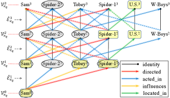
Non-interpretable. We show the computation graphs of GraIL and RED-GNN in the yellow space and green space respectively in Figure 7. Even though attention is applied in the GNN framework, how the weights cooperate in different layers is unclear. Thus they did not provide interpretation and nor can we come up a way to interpret the reasoning results in GraIL.
Empirical evidence. To show that GraIL fails to learn the relational structures, we conduct a tiny ablation study here. Specifically, we change the message function in GraIL from
where . This removes the relation when aggregating edges to only focus on graph structures.
We name this as GraIL no rel. The results are shown in Table 6. We observe that the performance decay is really marginal if relation is removed in the edges. This means that GraIL mainly learns on the graph structures and the relations play little role in. Thus, we claim that GraIL fails to learn the relational dependency in the ill-defined enclosing subgraph.
We also change the aggregation function in RED-GNN from (3) to
where is shared in the same layer, to remove the relation on edges. We denote this variant as RED-no rel. Note that RED-no rel is different from the variant Attn-w.o.- in Table 4. As in Table 6, the performance drops dramatically. RED-GNN mainly relies on the relational dependencies in edges as evidence for reasoning.
| methods | WN18RR (V1) | FB15k-237 (V1) | NELL-995 (V1) |
|---|---|---|---|
| GraIL no rel | 0.620 | 0.255 | 0.475 |
| GraIL | 0.627 | 0.279 | 0.481 |
| RED-no rel | 0.557 | 0.198 | 0.384 |
| RED-GNN | 0.701 | 0.369 | 0.637 |
Appendix C Proofs
C.1. Proposition 1
We prove this proposition from the bi-directions such that and .
Proof.
First, we prove that .
As in step-7 of Algorithm 1, is defined as . Thus we have and also .
Second, we prove that .
We use proof by contradiction here. Assume that is wrong, then there must exist and . In other words, there exists an edge that can be visited in steps walking from , but not in any r-digraph . Based on Def. 2 of r-digraph, then, will be an edge that is steps away from but does not belong to the -th triple of any relational paths , this is impossible. Therefore, we have .
Based on above two directions, we prove that . ∎
C.2. Proposition 2
Given a query triple and , when , it is obvious that in both Algorithm 1 and Algorithm 2. For , we prove by induction. We denote as the representations learned by Algorithm 1 and as the representations learned by Algorithm 2. Then, we show that for all and .
C.3. Theorem 1
Proof.
Based on Definition 2, any set of relational paths are contained in the r-digraph .
Denote as the r-digraph constructed by . In each layer, the attention weight is computed as
Then, we prove that can be extracted from the -th layer and recursively to the first layer.
-
•
In the -th layer, denote as the set of the triples , whose attention weights are , in the -th layer of . Based on the universal approximation theorem (Hornik, 1991), there exists a set of parameters that can learn a decision boundary that if and otherwise . Then the -th layer of can be extracted.
-
•
Similarly, denote as the set of the triples that connects with the remaining entities in the -th layer. Then, there also exists a set of parameters that can learn a decision boundary that if and otherwise not in. Besides, and are independent with each other. Thus, we can extract the -tfh layer of .
-
•
Finally, with recursive execution, can be extracted as the subgraph in with attention weights .
∎