Knot Dynamics
Abstract
The paper studies the dynamics of knots under self-repulsion produced by artificial charges placed on the curve in space representing the knot.
1 Introduction
It is the purpose of this paper to ask questions about the dynamics of knots under self-repulsion.
A knot is arranged in three dimensional space so that it is coated with a mathematical version of electrical charge so that it evolves to
geometric positions that minimize its energy under constraints that maintain its total length. Will such evolutions result in the unknotting of
loops that are topologically unknotted? What are the forms of extermal positions in such evolutions?
We will give a guided tour of computer experiments that can be performed in the quest for answers to these questions. In the course of our specific computer exploration we use
the knot theory of rational knots and rational tangles [5] to produce classes of unknots with complex initial configurations that we call hard unknots and corresponding
complex configurations that are topologically equivalent to simpler knots. We shall see that these hard unknots and complexified knots give examples that do not reduce in the experimental
space of the computer program. That is, we find unknotted configurations that will not reduce to simple circular forms under self-repulsion, and we find complex versions of knots that will not
reduce to simpler forms under the self-repulsion. It is clear to us that the phenomena that we have discovered depend very little on the details of the computer program as long as it
conforms to our general description of self-repulsion. Thus, we suggest on the basis of our experiments that sufficiently complex examples of hard unknots and sufficiently complex examples
of complexified knots will not reduce to global minimal energy states in self-repulsion environments. In the course of the paper we will make the character of these examples precise.
It is our challenge to other program environments to verify or disprove our assertions.
To make this challenge quite specific, here is a family of examples. Let
in the notation of Section 3 of this paper. is a diagram for an unknot.
The example is shown in Figure 17 and Figure 18. We conjecture that any algorithm based only on self-repulsion will be unable to unknot for some natural number value for
In this example, our version of KnotPlot is unable to unknot
More generally, again using the notation of Section 3, we have an infinity of unknots in the form where is a rational tangle in continued fraction form, and is the truncate of T obtained by removing the last term of These unknotted configuratons provide a wealth of inputs for knot dynamical experiments.
In Section 3 we explain how to create complex configurations of given knot types by the same method.
Having made this challenge, we point out that in [12] refined methods of gradient descent provide ways in which many examples that we do not reach with our methods can be unknotted.
And in [9] the BFACF algorithm [8] is used to strong effect. The challenge is given to all of these more powerful algorithms as well.
A knot is represented by a (cyclic) sequence of points in three dimensional space
In computer graphics the points can be shown and edges can connect point with point and of course with Another computer
graphic option is to enclose the resulting piecewise linear curve with tube so that the knot appears as a smooth tube with a chosen diameter. We make use of the computer program
KnotPlot [10] created by Robert Scharein, and we thank him for numerous conversations about the use of this program, and for modifying the program to facilitate the use of
tangles and rational knots. We shall refer to KnotPlot when speaking of experiments
and examples produced in the course of the paper.
A knot undergoes dynamics of self-repulsion in the computer program by a recursion involving forces of order ( is the distance between a chosen pair of points on the knot) applied to all pairs of non-adjacent points in the sequence of points that define the knot (see above).
The recursion is controlled so that the knot-type of the space curve does not change from step to step. We can calcluate the Simon Energy [13]. The Simon Energy is the sum of over all pairs of distinct points in the list of points in three dimensional space that describes the knot.
The KnotPlot program minimizes this energy by self-repulsion forces of order The Simon Energy corresponds directly to forces of the form
One can examine many aspects of the knot dynamics. Knots and links evolve into special geometric configurations that are not predictable beforehand.
One often finds that unknotted curves will unfold and become simplified into curves that are nearly flat circles. In some cases the force field cannot undo unknots.
The final configuration can depend upon the starting configuration and upon degrees of perturbation that are allowed in the process of evolution.
The program we use allows, in addition to the
repulsion forces, an attraction of nearby points via spring-forces (using an analog of Hooke’s Law) [11].
The balance of the spring and repulsion forces can be used to facilitate experiments.
We will give examples of all these phenomena.
2 Moving Down Energy Gradients
We begin with a relatively flat representation of the trefoil knot, a torus knot of type Generally we consider torus knots of type where and are relative prime positive
integers. Such a knot winds around a standardly embedded torus in three-space times around the meridian direction and times around the longitude direction. It is a fact that a torus knot
of type is topologically equivalent to a torus knot of type We shall write for a torus knot of type and so write that and are topologically equivalent. We shall see this equivalence emerge in the dynamics.
In Figure 1 we see the initial representation of In Figure 2 we see the result of the trefoil after it has reached self-repulsion stability. At this point the trefoil configuration has
calculated Simons energy The Simons energy is computed by using the fact that the knot we see is represented by a collection of points in three dimensional Euclidean space as shown in Figure 3. The Simons energy is the sum of ranging over all pairs of points in this configuration where is the Euclidean distance between the points
and The Simon energy corresponds classically to the force field with exponent but it is convenient to track this energy even when using other force functions.
In Figure 4 we see the initial state for a torus knot of type Topologically, a torus knot of type is equivalent to one of type but geometrically this is quite a different starting position. In one case the curve goes around the torus longitudinally twice and meridianally three times. This is reversed to three and two in the second case. We now examine how the repulsion dynamics worked on the In Figure 5 we see the self-repelled torus knot in what appears to be a stable position. Experimentally this configuration is
stable when using the undamped program in KnotPlot. Undamped means that the springs that are available between successive nodes in the model are not operation (in the sense that the spring constant is high and the springs are hence fully contracted). The energy level of this configuration is , considerably higher than the minimum we found for the knot. Now we have the opportunity to perturb this configuration by using the program in its undamped form. Then the springs are free to contract and expand, letting the energy move into kinetic energy of motion for the configuration. In Figures 6 7 8 9 we see that indeed the undamped evolution results in an oscillation that swings arcs of the knot around and lets it fall into the lower energy configuration of the trefoil knot.
Figures 10 11 12 13 14 15 illustrate the descent of a torus knot. The resulting energy minimum is Note that the internal twist
in the knot collapes in the course of this evolution. The same collapse will be observed for torus knots with
If one uses the undamped descent for a long time, then for the the resulting configuration does not change when the undamped evolution is made available.
If one runs the damped evolution for a short time, then the result will be similar to our evolution with the trefoil knot and an exchange of kinetic energy takes the knot to the same configuration as
the descent of the torus knot. We illustrate the final descent configuration for a torus knot in Figure 16.
In Figure 17 we illustrate an initial position for an unknot of type where we will explain this notation below. The Figure 18 shows the result of the undamped evolution of this knot. It has not become unknotted and no application of the undamped program will unknot it at any point in the process. This is an eperimental example of an unknnotted curve that fails to become unknotted in the force field of the Knotplot program. We conjecture that this phenomenon is not specific to this program but rather that some unknots of the form
will not be able to evolve to simple circles in any forcefield of this kind. The reader is advised to experiment with these examples. We explain the corresponding tangle theory in the next section.
The knot shown in Figure 19 is obtained by the same techniques as the previous two figures. It is of type and is equivalent to a figure eight knot as we will explain in the next section.It will not reduce any further in the KnotPlot environment either via undamped or damped evolution. In fact, as we will see in then next section, we have an infinite collection of figure eight knots in the forms and for greater than we have the empirical result that they all have local energy minima , increasing with the value of in the KnotPlot environment.
We conjecture that this phenomenon is qualitatively the same in any force field environment for knot repulsion.
 |
 |
 |
 |
 |
 |
 |
 |
 |
 |
 |
 |
 |
 |
 |
 |
 |
 |
 |
3 Hard Knots and Collapsing Tangles
Before we begin the details of this section, the reader should view Figure 26. There is illustrated a diagram and a sequence of steps that show that the diagram is
unknotted. This is the type of unknot that we have discussed in the previous section. In order to systematically construct configurations of this type, that are complex and yet unknotted, we
develop an algebraic language of tangles in the present section of the paper. For complete information about all aspects of this discussion we recommend that the reader consult
the paper [5].
In this section we give background in terms of a theory of tangles for constructing the unknots and knots in collapsible states.
We begin with the definition of a tangle and the notions of combination of tangles (addition, star product, numerator and denominator) and how this leads to the tangle fraction, the notion of
rational tangles and rational knots and how these constructions are related to computer experiments.The notion of a tangle was introduced in 1967 by
Conway [1] in his work on enumerating and classifying knots and links.
A -tangle is a proper embedding of two unoriented arcs and a finite number of circles in a -ball
so that the four endpoints lie in the boundary of . A tangle diagram is a regular projection
of the tangle on an equatorial disc of A rational tangle is a special case of a -tangle obtained by applying consecutive twists
on neighbouring endpoints of two trivial arcs. Such a pair of arcs comprise the or tangles
as shown in Figure 21, depending on their position in the plane. We shall say that the rational tangle is in twist form when it is obtained by such successive twists of adjacent strands. For example see Figure 20 where we show a tangle in the center of the figure that is obtained by
first starting with a horizontal 3-twist ( in Figure 21 and then twisting two vertical strands negatively twice and then twisting two horizontal strands positively twice.
Tangles obtained recursively from the untwisted tangles and of Figure 21 are called rational tangles.
Note that in Figure 21 we have indicated horizontal twists by bracketed integers and vertical twists by reciprocal integers including the convention that
In Figure 22 we show tangle operations , , and These are called addition, star product and rotation of tangles. The rotation operation has the effect of turning the tangle by ninety degrees in the plane. Note that twisting horizontal strand times is the same as forming and twisting vertical strands times is the same as forming . Thus we can describe the tangle in Figure 20 as (.
It turns out that one can associate to any tangle a fraction with values in the rational numbers plus the formal value and that this fraction satisfies the following rules with
respect to addition, star product and rotation. Here denote the mirror image tangle, obtained by switching all the crossings of
Once we assume that these rules determine the fractions of rational tangles.
-
1.
-
2.
-
3.
-
4.
The second property of the fraction for the star product is a conseqence of first property for addition, using the third property that tells us that the fraction of a rotate is the negative reciprocal of
the fraction of the original tangle. Note that it follows from these rules that and that and that
This is the formula for the fraction of a tangle with an extra vertical twist at the bottom. From this formula we see that the fraction of a rational tangle will be represented by a continued fraction. For example,
For this reason it is useful to denote rational tangles by just writing a corresponding continued fraction.
 |
 |
 |
 |
 |
 |
 |
 |
 |
 |
 |
 |
 |
 |
We will illustrate this with an example. In Figure 23 we illustrate these properties by starting with the tangle from Figure 20 and noting that is a sum of the form where We could directly use the rules above to compute as follows.
In the Figure 23 we denote and use property above to rotate the tangle and then use property to complete the calculation of without using property In the rest of the figure we note that has a positive continued fraction expansion as The last symbol, is the symbol for this continued fraction. Thus
and more generally
Thus we shall from now on use the continued fraction written numerically to indicate the corresponding rational tangle. Thus will be our notation for the tangle diagram at the bottom of
Figure 23. Note that topologically this tangle is equivalent to These symbols represent the same numerical fraction and they each represent specific diagrams for rational tangles. The Figure 23 gives the reader enough information to see that these two tangles are topologically equivalent. That is, the reader can take as an exercise to deform the tangle
to the tangle by an isotopy that does not move any arcs over the endpoints of the tangle, while leaving the endpoints fixed.
John Horton Conway proved that two rational tangles are topolgically equivalent if and only if they have the same fraction. See [1, 5, 6, 7] for statements and proofs of the Conway Theorem. The key to our approach to proving the Conway Theorem, in these cited papers, is the insight that any continued fraction tangle with a mixture of signs such as
is not an alternating weave, and can be simplified by standard isotopies (swinging arcs that go over or under consecutive crossings) until it is alternating. The rational form of the tangle is
retained under such isotopies, and the final alternating form corresponds to an entirely positive (or entirely negative) sequence such as The only positive or only negative sequence is uniquely obtained from the fraction itself
by Euclid’s algorithm. We give no more details here, but refer to our papers.
Note that Thus These sequential symbols are useful for handling rational tangles and continued fractions. Note also that when we
draw the twists occur from right to left. Thus in Figure 23 we illustrate and the occurs on the right in the diagram.
In Figure 24 we illustrate a useful fact about about tangles. If is a tangle and we apply rotation to it twice it will be rotated by 180 degrees. It turns out that for rational tangles, one can pick them up, rotate them by 180 degrees and they are topologically unchanged. The figure illustrates one case of the internal topological rotations that accomplish this fact.
The next operation we need is the numerator construction that converts a tangle to a knot of link by connect the top strands to one another and the bottom strands to one another.
See Figure 20 for an illustration of the numerator operation and its so-called corresponding denominator operation. A theorem of Schubert (See [LKS]) gives a classification of
the rational knots obtained as numerators of rational tangles. We do not need the full Schubert Theorem here but refer to [7] for the reader who wants more information about it.
In Figure 25 we illustrate the formula Actually this is simply an identity for tangles, but it is often occurring inside a numerator closure. Note that algebraically this is just the cancellation of with but topologically it can be interpreted as the result of a rotation that involves the intermediate tangle Such rotations occur in
manipulating rope models and in the motions of curves in the force fields we have considered in the first section of the paper.
Now we are in position to look at Figure 26 again. Note that the diagram indicated is and so the and cancel is in the previous paragraph. Again one can see this by an internal rotation in the numerator closure. The rest of the figure illustrates how this configuration is unknotted.
We can note that if and the tangle obtained by reversing all the terms in then and are topologically equivalent knots. The Figure 27 will give the reader an appreciation of this fact. In that figure we illustrate how by representing each of these tangles in a
partially braided form. The reader can take as an exercise to see that any continued fraction template for a rational tangle can be put into such a braided form.
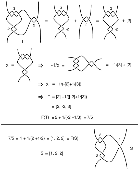
Figure 28 illustrates for and We have the basic fact that the numerator of the sum of two rational tangles and is topologically equivalent to the numerator of a rational tangle that is constructed from the two of them. Given and let be defined by the formula
Then is topologically equivalent to In order to see this topological equivalence the Figure shows how to rotate and isotope so that it is clearly equivalent to But we know that for any So this gives the desired result. Thus in Figure 28 we see that
The rotation that we see in in Figure 28 is the key to producing many diagrams of the unknot that can be difficult for the dynamics of the program to undo. The basic result is this: Let and Then is topologically equivalent to the unknot. Figure 26 illustrates how this works. The tangle has just one less term than the tangle and is obtained from it by removing the last term of We call the truncate of In the figure the reader should be able to see that the from and the from flank a tangle and allow a rotation that cancels these terms and then brings and into cancelling position. This continues recursively and allows the knot to unwind and become unknotted. To see this result in tangle terms the following identity is of use:
where this equality can be read as topological equivalence of tangles, or as identity of continued fractions. For example, in fractions we have
The unknotting is then mirrored in a bit of algebra. For example
and is unknotted.
By the same token, we can arrange tangle diagrams that collapse to certain knots. For example,
This means that we can give the dynamics program tangled versions of knots and unknots and perform experiments to see if the program
will undo the unknots and collapse the complexified knots to simpler forms.
3.1 Collapse Examples
Notation. We make the following definitions. Let with ’s in the continued fraction sequence.
Let This is the notation we have used in the first section of the paper. Thus Figure 17 and Figure 18 give images
for a configuration that we know is unknotted from the above construction. These figures show that the KnotPlot program takes to a stable state
that is still entangled. The second instance is Figure 19 where we show how also has a complex stable state. By our discussion below we will see
that for , Thus and this is a Figure Eight knot.The upshot of these constructions is that we can give
infinitely many examples of configurations that are either knotted or unknotted but have complex stable states in the force field algorithm of KnotPlot.
To prove that consider an example:
Thus the proof of this fact follows from the work we have already done, plus the use of this compressed notation.
We will also write so that the can indicate consecutive ’s in the tangle. Then we have the basic result that
is isotopic to
where can be replaced by any continued fraction tangle.
This result follows by the same reasoning as we have outlined above, and it provides a large collection of starting configurations for testing a self-repulsion program.
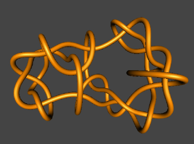
Our last example illustrates all the principles in this section. The basic knot we work with is the rational knot
illustrated in its initial form in Figure 30 and it its final fully repelled form in Figure 31.
In Figure 32 we show the initial form of
In Figure 33 we show the final self-repelled form that occurs from this beginning.
We see that in this case does not reduce to the minimal form of in the KnotPlot environment.
It is our conjecture that no environment of this type will fully reduce all of the configurations and we challenge users or designers of other
programs to experiment with this family of configurations of the knot There is, of course, nothing special about the choices we have made here.
The phenomenon of non-collapse will occur for sufficiently large complexifications of any knot or unknot.
References
- [1] J.H. Conway, An enumeration of knots and links and some of their algebraic properties, Proceedings of the conference on Computational problems in Abstract Algebra held at Oxford in 1967, J. Leech ed., (First edition 1970), Pergamon Press, 329-358.
- [2] A. Henrich, L. H. Kauffman, Unknotting unknots, Amer.Math. Monthly May 2014, pp. 379-390.
- [3] L.H. Kauffman, State Models and the Jones Polynomial, Topology 26 (1987), 395–407.
- [4] L. H. Kauffman, “Knots and Physics”. Fourth edition. Series on Knots and Everything, 53. World Scientific Publishing Co. Pte. Ltd., Hackensack, NJ, 2013. xviii+846 pp. ISBN: 978-981-4383-01-1.
- [5] L. H. Kauffman and S. Lambropoulou, Hard knots and collapsing tangles, in in “Introductory Lectures in Knot Theory”, K&E Series Vol. 46, edited by Kauffman, Lambropoulou, Jablan and Przytycki, World Scientiic 2011, pp. 187 - 247.
- [6] L.H. Kauffman, S. Lambropoulou, On the classification of rational tangles, Advances in Applied Math, 33, No. 2 (2004), 199 237.
- [7] L.H. Kauffman, S. Lambropoulou, On the classification of rational knots. L’Enseignement Mathématiques, 49, (2003), 357-410.
- [8] E. J. van Rensburg, .A. Rechnitzer, BFACF-style algorithms for polygons in the body-centered and face-centered cubic lattices. J. Phys. A 44 (2011), no. 16, 165001, 25 pp.
- [9] R. Scharein, K. Ishihara, J. Arsuaga, Y. Diao, K. Shimokawa, M. Vazquez, Bounds for the minimum step number of knots in the simple cubic lattice. J. Phys. A 42 (2009), no. 47, 475006, 24 pp. 92D10
- [10] R. Scharein, KnotPlot (program available from the web), http://wren.pims.math.ca/knotplot.
- [11] R. Scharein, Interactive Topological Drawing, PhD Thesis, Department of Computer Science, University of British Columbia, March 1998.
- [12] P. Reiter and H. Schumacher, Sobolev Gradients for the Mobius Energy May 18, 2020, arXiv:2005.07448.
- [13] J. K. Simon, Energy functions for polygonal knots. Journal of Knot Theory and Its Ramifications, 3(3):299 320, 1994.