Khovanov homology and exotic -manifolds
Abstract.
We show that the Khovanov-Rozansky skein lasagna module distinguishes the exotic pair of knot traces and , an example first discovered by Akbulut. This gives the first analysis-free proof of the existence of exotic compact orientable -manifolds. We also present a family of exotic knot traces that seem not directly recoverable from gauge/Floer-theoretic methods. Along the way, we present new explicit calculations of the Khovanov skein lasagna modules, and we define lasagna generalizations of the Lee homology and Rasmussen -invariant, which are of independent interest. Other consequences of our work include a slice obstruction of knots in -manifolds with nonvanishing skein lasagna module, a sharp shake genus bound for some knots from the lasagna -invariant, and a construction of induced maps on Khovanov homology for cobordisms in .
1. Introduction
The revolutionary work of Donaldson and Freedman in the s revealed a drastic dichotomy between the topological and smooth category of manifolds in dimension . Since then, constant efforts are made to find exotic pairs of -manifolds.
A pair of smooth -manifolds and is said to be exotic if they are homeomorphic but not diffeomorphic. In preferable cases, showing two -manifolds are homeomorphic boils down to checking some algebraic topological invariants agree, thanks to Freedman’s fundamental theorems [freedman1982topology]. Showing that they are non-diffeomorphic usually involves showing some gauge-theoretic or Floer-theoretic smooth invariants (Donaldson invariants [donaldson1990polynomial], Seiberg-Witten invariants [seiberg1994monopoles], Heegaard Floer type invariants [ozsvath2004holomorphic], and various variations/generalizations) differ. To date, all detection of compact orientable exotic -manifolds depends heavily on analysis, mostly elliptic PDE. We present the first analysis-free detection result.111For a noncompact example, an exotic can be constructed from a topologically slice but not smoothly slice knot. Such knots can be detected by Freedman’s result [freedman1982topology] and Rasmussen’s -invariant [rasmussen2010khovanov] from Khovanov homology. For nonorientable examples, Kreck [kreck2006some] showed and form an exotic pair using Rochlin’s Theorem, and indeed exotic ’s were constructed by Cappell-Shaneson [cappell1976some] (shown to be homeomorphic to later in [hambleton1994nonorientable]).222Exotic surfaces in -manifolds were also known to be detectable by Khovanov homology [hayden2021khovanov].
The relevant smooth invariant in our story is the Khovanov-Rozansky skein lasagna module (Khovanov skein lasagna module for short) defined by Morrison-Walker-Wedrich [morrison2022invariants], which is an extension of a suitable variation of the classical Khovanov homology [khovanov2000categorification] via a skein-theoretic construction. It assigns a tri-graded (by homological degree , quantum degree , and homology class degree below) abelian group
to every pair of compact oriented smooth -manifold and framed oriented link on its boundary. When is the empty link we simply write for the skein lasagna module.
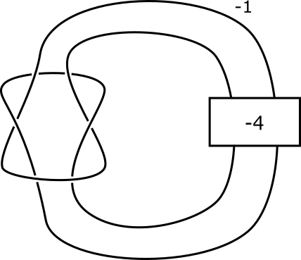
The -trace on a knot , denoted , is the -manifold obtained by attaching an -framed -handle to along . Our main theorem shows that the -traces on the mirror image of the knot and the Pretzel knot , namely
have non-isomorphic skein lasagna module.

Theorem 1.1.
The graded modules and are non-isomorphic over . Therefore, and form an exotic pair of -manifolds. In fact, even their interiors are exotic.
The exotic pair was first discovered by Akbulut [akbulut1991exotic, akbulut1991fake]. The fact that are homeomorphic is more or less standard: a sequence of Kirby moves shows and are homeomorphic and a suitable extension of Freedman’s Theorem [freedman1982topology, boyer1986simply] then implies and are homeomorphic. On the other hand, the fact that are not diffeomorphic was detected by an intricate calculation of Donaldson invariants. Later, the result was reproved by Akbulut-Matveyev [akbulut1997exotic, Theorem 3.2] using a simplified argument which essentially says is Stein (since the maximal Thurston-Bennequin number of is ) while is not (since is slice). This latter proof is elegant, yet still depends heavily on calculation of Seiberg-Witten invariants of Stein surfaces, as well as deep results of Eliashberg [eliashberg1990topological] and Lisca-Matić [lisca1997tight]. In comparison, our proof of Theorem 1.1 depends on the much lighter package of Khovanov homology, which is combinatorial in nature.
Since the Khovanov skein lasagna module over a field of a connected sum or boundary connected sum of -manifolds is equal to the tensor product of the Khovanov skein lasagna modules of the components, a fact proved in [manolescu2022skein], and remain exotic after (boundary) connected sums with any -manifolds with nonvanishing skein lasagna module (at least when the support of is small in a suitable sense). Such tricks lead to many new exotic pairs. We write down some explicit examples in the following corollary to give the reader a flavor of what can be proven. For more choices of such candidates of connected summands one may look into Section 6.
Corollary 1.2.
The -manifolds and form an exotic pair if and . The exotica remain under connected sums or boundary sums with any copies of , , , and the negative manifold. The exotica also remains upon further taking the interiors of the pair.
Anubhav Mukherjee informed us that most of these variations seem also achievable via gauge/Floer-theoretic methods and topological arguments. However, below we present a family of exotic knot traces generalizing Theorem 1.1 that seems not directly recoverable from other methods. Let and be satellite patterns drawn as in Figure 2, and , be the corresponding satellite knots with companion knot . These satellite patterns were first studied by Yasui [yasui2015corks]. Let denote the Rasmussen -invariant of .
Theorem 1.3.
If a knot has a slice disk in and are two integers satisfying
then and form an exotic pair. Their interiors are also exotic.
In the special case when is the unknot, , is the trivial slice disk of in , and , , Theorem 1.3 recovers Theorem 1.1. One can also construct more exotic pairs in the spirit of Corollary 1.2 by taking connected sums of these examples and other standard manifolds appearing in that corollary.
Now we turn to some explicit calculations of and other applications. Some topological applications we derived can indeed be proved in other ways, but our approach provides the first analysis-free proofs. We also give a proof of Theorem 1.1 in Section 1.5, assuming some results stated.
Throughout this paper, all -manifolds are assumed to be smooth, compact, and oriented. All surfaces are oriented and smoothly and properly embedded. In the current section, many statements are presented in a specialized form. In such cases, we indicate the corresponding generalizations in the parentheses after the statement numbers.
1.1. A vanishing result and slice obstruction
For a knot , let denote its maximal Thurston-Bennequin number. We have the following vanishing criterion for the Khovanov skein lasagna module.
Theorem 1.4.
If the knot trace for some knot and framing embeds into a -manifold , then for any .
For example, since contains an embedded sphere with self-intersection , we see the -trace of the unknot embeds into , implying . This answers a question of Manolescu (see [sullivan2024kirby, Question 2]), generalizing one main Theorem of Sullivan-Zhang [sullivan2024kirby, Theorem 1.3] and answering [sullivan2024kirby, Question 3] in the affirmative.
The folklore trace embedding lemma says that embeds into if and only if is -slice in , i.e. there is a framed slice disk in of the -framed knot . Therefore, the contrapositive of Theorem 1.4 can be phrased as follows.
Corollary 1.5.
Suppose for some . If a knot is -slice in , then .∎
1.2. Lee skein lasagna modules and lasagna -invariants
In the construction of the Khovanov skein lasagna module, the relevant TQFT (the Khovanov-Rozansky homology) enters only at the very last step. We could replace this TQFT by its Lee deformation [lee2005endomorphism], and define an analogous notion of a Lee skein lasagna module of a -manifold with link , denoted . It is a -vector space equipped with a homological -grading, a quantum -grading, a homology class grading by , and a quantum -filtration (where has filtration degree ), with the caveat that a nonzero vector can have quantum filtration degree .
We show in Section 4 that the structure of , except for the quantum filtration, is determined by simple algebraic data of . Moreover, we extract numerical invariants from the quantum filtration structure333The authors are aware that the recent paper [morrison2024invariants] by Morrison-Walker-Wedrich has an independent proof of a part of this structural result (except addenda (3) and (4)), stated in a more general form. They extract slightly different invariants from the filtration structure, which gives somewhat less information than ours in the case. Moreover, our invariants generalize Rasmussen -invariants for links and enjoy nice functorial properties.. For the purpose of exposition, in the current section we assume is the empty link. Let denote the quantum filtration function.
Theorem 1.6.
(Theorem 4.1) The Lee skein lasagna module of a -manifold is with a basis consisting of canonical generators , one for each pair . Moreover,
-
(1)
has homological degree ;
-
(2)
has homology class degree ;
-
(3)
, have quantum degrees , , respectively;
-
(4)
, which also equals if in .
Definition 1.7.
(Definition 4.6) The lasagna -invariant of at a homology class is
The lasagna -invariants of thus define a smooth invariant .
The genus function of a -manifold , defined by
captures subtle information about the smooth topology of . Like the classical -invariant [rasmussen2010khovanov, beliakova2008categorification], which provides a lower bound on the slice genus of links, the lasagna -invariants provide a lower bound on the genus function of -manifolds.
Theorem 1.8.
(Theorem 4.7(6) and Corollaries after) The genus function of a -manifold has a lower bound given by
Unlike the classical -invariant, the lasagna -invariants are not directly computable from link diagrams. However, we are able to compute them in some special cases. We indicate one special case where Theorem 1.8 does provide useful information.
The -shake genus of a knot is defined by , where is a generator of . Clearly, , but the inequality may not be strict [akbulut19772, piccirillo2019shake]. Theorem 1.8 specializes to a shake genus bound
| (1) |
Theorem 1.9.
-
(1)
If is concordant to a positive knot, then for we have where is the Rasmussen -invariant of . Thus
-
(2)
If is a concordance from to a positive knot , then for we have . Thus
Remark 1.10.
The computation of shake genus in Theorem 1.9(1) also follows from the following two facts:
-
(i)
The adjunction inequality for Stein manifolds [lisca1997tight], which implies
(2) for any Legendrian representative of with . When , take to be a stabilization that maximize , of a max tb representative of . Then the right hand side agrees with for positive knots [tanaka1999maximal, Theorem 2].
-
(ii)
Two concordant knots have the same shake genus (by an easy topological argument).
Lasagna -invariants also obstruct embeddings between -manifolds in the following sense.
Proposition 1.11.
If is an inclusion between two -manifolds, then for any class ,
1.3. Nonvanishing result for -handlebodies from lasagna -invariants
The Khovanov homology of a link admits a spectral sequence to its Lee homology. In particular, in every bidegree, the rank of the Khovanov homology is bounded below by the dimension of the associated graded vector space of the Lee homology. Although we are not able to define a spectral sequence from to , we do have a rank inequality when is a -handlebody. Let denote the associated graded vector space of a filtered vector space .
Theorem 1.12.
If is a -handlebody, then in any tri-degree ,
In particular, if the quantum filtration on is not identically , then .
We state a comparison result for Lee skein lasagna modules of -handlebodies, which can sometimes be used as a nonvanishing criterion for Khovanov skein lasagna modules in view of Theorem 1.12.
Proposition 1.13.
(Proposition 5.3) Suppose (resp. ) is a -handlebody obtained by attaching -handles to along a framed oriented link (resp. ). If is framed concordant to , then as tri-graded, quantum filtered vector spaces. Under the identification induced by a link concordance, and have equal lasagna -invariants.
1.4. Nonvanishing result for -handlebodies from link diagram
Using a diagrammatic argument, in Section 5.4, we prove a nonvanishing result for -handlebodies with sufficiently negative framings. For the ease of exposition, here we only state the case for knot traces. Let be the minimal number of negative crossings among all diagrams of a knot .
Theorem 1.14.
(Theorem 5.5) Let be a knot and be its -trace.
-
(1)
If , then and
-
(2)
If is positive, then for , , . For ,
1.5. Proof of Theorem 1.1
Since is a positive knot with , by Theorem 1.9(1) we have . On the other hand, is slice, thus . This shows and are non-diffeomorphic, without actually calculating .
We still need to argue the Khovanov (and indeed Lee) skein lasagna modules of actually differ. Apply Theorem 1.14(2) to , we obtain ,
Apply Theorem 1.14(2) to the unknot, and then Proposition 1.13 to and the unknot, we obtain , and
where the first containment follows from Theorem 1.12. In particular, .∎
1.6. Example: Khovanov and Lee skein lasagna module of
As an example, we note that the recent work by the first author [ren2023lee] has the following implications on the Lee and Khovanov skein lasagna modules for .
Proposition 1.15.
The lasagna -invariants of are given by . The associated graded vector space of the Lee skein lasagna module of is given by for
and in other tri-degrees. Moreover, for ,
A consequence of this result, together with some properties of lasagna -invariants, is the following.
Corollary 1.16.
If a -manifold admits an embedding for some , then , with equality achieved if is a -handlebody and . In particular, for , and for if .
It is also worth pointing out that Conjecture 6.1 in [ren2023lee] is equivalent to a complete determination of the Khovanov skein lasagna module of (see Conjecture LABEL:conj:-CP2).
If is an oriented cobordism in between two oriented links , the last part of Proposition 1.15 enables us to define an induced map
between ordinary Khovanov homology of and , at least over a field and up to sign, with bidegree . We carry out this construction in more details in Section LABEL:sbsec:Kh_CP2_cob.
1.7. A conjecture for Stein manifolds
Many similarities between skein lasagna modules and other gauge/Floer-theoretic smooth invariants appear. However, a serious constraint for our computation is that we were not able to produce any -manifold with that has finite lasagna -invariants or nonvanishing Khovanov skein lasagna module. In fact, if one were able to find a simply-connected closed -manifold with that has , then is an exotic closed -manifold, as it has nonvanishing while its standard counterpart (some ) has vanishing .
To pursue this thread, we propose the following conjecture, which seems plausible and desirable.
Conjecture 1.17.
If is a knot and for some , then and . In particular, . More generally, any Stein -handlebody has and nonvanishing Khovanov skein lasagna module.
1.8. Organization of the paper
In Section 2, we review the theory of Khovanov skein lasagna modules, expanding on a few properties, as well as making some new comments on the skein-theoretic construction. In the short Section 3, we prove Theorem 1.4 by applying a bound on Khovanov homology by Ng [ng2005legendrian], and we give some examples of -manifolds with vanishing Khovanov skein lasagna module.
In Section 4, we develop the theory of Lee skein lasagna modules and lasagna -invariants, which can be thought of as a lasagna generalization of the classical theory by Lee [lee2005endomorphism] and Rasmussen [rasmussen2010khovanov] for links in . A generalization of Theorem 1.6, in particular the definition of canonical Lee lasagna generators, is presented in Section 4.1. The behavior of canonical Lee lasagna generators under morphisms is given in Theorem 4.5 in Section 4.2. Building on these results, in Section 4.3 we define and examine the lasagna -invariants, generalizing Definition 1.7, Theorem 1.8, and Proposition 1.11.
In Section 5, we make use of a -handlebody formula by Manolescu-Neithalath [manolescu2022skein] to prove nonvanishing results for Khovanov and Lee skein lasagna modules of -handlebodies. In Section 5.1, we prove Theorem 1.12 which shows that finiteness results for the quantum filtration of Lee skein lasagna modules imply nonvanishing results for Khovanov skein lasagna modules. In Section 5.2 we prove a generalization of Proposition 1.13 and in Section 5.3 we show that lasagna -invariants can be expressed in terms of classical -invariants of some cable links. Finally, in the somewhat technical Section 5.4, we prove a vast generalization of the diagrammatic nonvanishing criterion Theorem 1.14.
Finally, in Section 6, we give examples and applications, mostly to the theory and tools developed in Section 4 and Section 5. This includes proofs of Corollary 1.2, Theorem 1.3, Theorem 1.9, and an expanded discussion of Section 1.6. Other discussions include a proof that -invariants of cables of the Conway knot can obstruct its sliceness, and that the Khovanov skein lasagna module over does not detect potential exotica arising from Gluck twists in .
Most of our developments are independent to proving Theorem 1.1. The readers only interested in Theorem 1.1 may want to look at its proof in Section 1.5 and delve into the corresponding sections. In particular, to distinguish the smooth structures of the pair in Theorem 1.1, one can read the first half of Section 2, certain statements in Section 4 (mainly Definition 4.6 and Corollary 4.13), Section 5.4, and Section 6.4. The minimal amount of theory needed to actually distinguish their Khovanov skein lasagna modules depends moreover on Section 5.1 and Section 5.2 (but not really on Corollary 4.13 and Section 6.4). Still, the statements in those sections are often much more general than needed for Theorem 1.1, which at times complicate the proofs.
Acknowledgement
We thank Ian Agol, Daren Chen, Kyle Hayden, Sungkyung Kang, Ciprian Manolescu, Marco Marengon, Anubhav Mukherjee, Ikshu Neithalath, Lisa Piccirillo, Mark Powell, Yikai Teng, Joshua Wang, Paul Wedrich, Hongjian Yang for helpful discussions. This work was supported in part by the Simons grant “new structures in low-dimensional topology” through the workshop on exotic -manifolds held at Stanford University December 16-18, 2023.
2. Khovanov and Lee skein lasagna modules
The Khovanov-Rozansky skein lasagna modules were defined by Morrison-Walker-Wedrich [morrison2022invariants]. In the first part of this section we review its construction, cast in a slightly different way, while defining its Lee deformation under the same framework. In Section 2.1, we begin with a general skein-theoretic construction of skein lasagna modules, using an arbitrary (stratified) TQFT for links in . In Section 2.2, we state a few properties of skein lasagna modules, most of which are essentially proved in [manolescu2022skein]. Only then, in Section 2.3, do we fix the TQFT in consideration to be either the Khovanov-Rozansky homology [morrison2022invariants] or its Lee deformation [lee2005endomorphism]. We state a few more computational results for these settings in Section 2.4.
The second part of the section is new, and can be skipped on a first reading. In Section 2.5, we identify the structure of the underlying space of skeins in the construction of Section 2.1. The proof will eventually be useful in Section 4.1 where we calculate the Lee skein lasagna module of a pair . Finally, in Section 2.6, we suggest a few variations of the skein-theoretic construction.
2.1. Construction of skein lasagna modules
444The formulation of our construction was motivated by a conversation with Sungkyung Kang.Let be a -manifold and be a framed oriented link on its boundary. A skein in or in rel is a properly embedded framed oriented surface in with the interiors of finitely many disjoint -balls deleted, whose boundary on is . That is, a skein in can be written as
| (3) |
The deleted balls are called input balls of the skein .
We define the category of skeins in , denoted , as follows. The objects consist of all skeins in rel . Suppose is an object as in (3) and is another object with input balls , . If and each either coincides with some or does not intersect any on its boundary, then the set of morphisms from to consists of pairs of an isotopy class of surfaces555We formally allow some components of to be curves on the boundaries of those . rel boundary with , , and an isotopy class of isotopies from 666In order for the surfaces to glue smoothly, one may assume throughout that all embedded surfaces have a standard collar near each boundary, and all isotopies rel boundary respect these collars. to rel boundary. We will suppress the isotopy and write for this morphism. If the input balls do not satisfy the condition above, there is no morphism from to . The identity morphism at is given by . The composition of two morphisms and is (together with the composition of isotopies).
Next we introduce an arbitrary (stratified) TQFT of framed oriented links in , by which we mean a symmetric monoidal functor from the category of framed oriented links in and link cobordisms in up to isotopy rel boundary, to the category of modules over a commutative ring , such that and is finitely generated for all links . Equivalently, is a functorial link invariant in satisfying the conditions in Theorem 2.1 of [morrison2024invariants]. At times we also assume is a field and is involutive, meaning that for a link and for a cobordism , where is the reverse cobordism.
Assign to every object of as in the notations before the -module which we denote by an abuse of notation , where each is a framed link. Assign to every morphism the morphism induced by the cobordism . Then defines a functor from the category of skeins in to the category of -modules.
The skein lasagna module of with respect to , denoted , can be now defined as
| (4) |
More explicitly,
| (5) |
where is the equivalence relation generated by linearity in , and for . A pair (or just if there’s no confusion) as in (5) is called a lasagna filling of .
The skein lasagna module is an invariant of the pair up to diffeomorphism. When , we write for short for . In this case, since all lasagna fillings and their relations appear in the interior of , is an invariant of .
2.2. Properties of skein lasagna modules
We state some properties of the skein lasagna modules, mostly following Manolescu-Neithalath [manolescu2022skein]. Although their paper dealt with the case when the TQFT is the Khovanov-Rozansky homology, the proofs remain valid in the more general setup. We remark that the more recent paper [manolescu2023skein] gives a formula for in terms of a handlebody decomposition of . However, we will not be using this result, so we refer interested readers to their paper.
Every object of represents a homology class in , whose image under the boundary homomorphism in the long exact sequence
is , the fundamental class of . If is a morphism, then . This means admits a grading by , which we write as
Of course, is nonempty if and only if the image of in is zero, i.e. is null-homologous in . From now on this will be assumed, since otherwise is trivially zero as there is no lasagna filling.
Proposition 2.1 (-handle attachments, [manolescu2022skein, Proposition 2.1]).
If is obtained from by attaching a -handle (resp. -handle) away from , then there is a natural surjection (resp. isomorphism) .∎
Proposition 2.2 (Connected sum formula, [manolescu2022skein, Theorem 1.4,Corollary 7.3]).
If the base ring is a field and is involutive, then there is a natural isomorphism
The same formula holds with the boundary sum replaced by the connected sum or the disjoint union.∎
Suppose is a pair and is a properly embedded separating oriented -manifold, possibly with transverse intersections with in some point set . Then cuts into two pairs and , where induces the orientation on and induces the reverse orientation, and are framed oriented tangles with endpoints . The framing and the orientation of restrict to a framing and an orientation of .
If is a framed oriented tangle with in the framed oriented sense, then is a framed oriented link in and is one in . A lasagna filling of and a lasagna filling of glue to a lasagna filling of in a bilinear way, inducing a map
| (6) |
Proposition 2.3 (Gluing).
The gluing map
is a surjection.
Proof.
Every lasagna filling of can be isotoped to intersect transversely in some tangle . ∎
Write . A framed surface with is a lasagna filling of (without input balls), thus putting its class in the second tensor summand of (6) defines a gluing map
| (7) |
The most useful cases of gluing might be when is closed, where , and are links. Still more specially, if is an inclusion of -manifolds, there is an induced map by gluing the exterior of to . For example, the map in Proposition 2.1 is defined this way.
The skein lasagna module with respect to refines the TQFT in the following sense.
Proposition 2.4 (Recover TQFT).
For a framed oriented link we have a natural isomorphism . If is a cobordism from to , then the gluing map agrees with under the natural isomorphisms.
Proof.
The statement on objects is proved in [morrison2022invariants, Example 5.6] and the statement on morphisms is a simple exercise. ∎
Finally, we remark that extra structures on the TQFT usually induce structures on the skein lasagna module . For example, suppose takes values in -modules with a grading by an abelian group , so that for a link cobordism , is homogeneous with degree for some independent of . Then the lasagna module inherits an -grading, once we impose an extra grading shift of in the definition of for a skein . Analogously, a filtration structure on induces a filtration structure on . The isomorphisms or morphisms stated or constructed in this section all respect the extra grading or filtration structure, with a warning that the gluing morphism in (7) has degree or filtration degree .
Remark 2.5.
In view of the gluing morphism (7) (in the special case and ), one is tempted to define a TQFT for framed oriented links in oriented -manifolds and cobordisms between them. Namely, for a -manifold and link , define
For a cobordism , define by taking the direct sum of the gluing maps .
However, the resulting modules are usually infinite dimensional. To obtain a finite theory, one has to either restrict the domain category (one extreme of which is to recover back the TQFT for links in again), or modulo suitable skein-theoretic relations on . We leave the exploration of these possibilities to future works.
2.3. Khovanov-Rozansky homology and its Lee deformation
In this paper we will take the TQFT in the skein lasagna construction to be the Khovanov-Rozansky homology or its Lee deformation. In this section we review some features of these TQFTs, partly also to fix the renormalization conventions and do some bookkeeping. We assume the reader is familiar with the classical Khovanov homology as well as its Lee deformation. See [khovanov2000categorification, lee2005endomorphism, rasmussen2010khovanov] for relevant backgrounds and [bar2002khovanov] for an accessible overview.
We follow the convention in [morrison2022invariants]. Khovanov-Rozansky homology is a renormalization of the Khovanov-Rozansky homology defined in [khovanov2008matrix] (and extended to -coefficient in [blanchet2010oriented]) that is sensitive to the framing of a link. Since conventionally most calculations have been done using the classical Khovanov homology [khovanov2000categorification], we write down explicitly the renormalization differences between it and the theory.
Let and denote the Khovanov-Rozansky homology and the usual Khovanov homology, respectively. Then for a framed oriented link , we have
| (8) |
where is the writhe of , and is the mirror image of . When we want to emphasize that we are working over a commutative ring , write and for the corresponding homology theories.
A dotted framed oriented cobordism in induces a map of bidegree which only depends on the isotopy class of rel boundary. Let denote the mirror image of . Then the identification (8) is functorial in the sense that is equal to under (8) up to sign. Since the classical Khovanov homology is only known to be functorial in up to sign, can be thought of as a sign fix and a functorial upgrade of .
Both the constructions of and depend on the input of the Frobenius algebra 777Strictly speaking, the construction of uses the formalism of foams, but for simplicity, our discussion stays in the classical Khovanov formalism throughout. with comultiplication and counit given by
Here has quantum degree in the case and in the case.
The Lee deformation of over [lee2005endomorphism] is the Frobenius algebra with
Using instead of defines the Khovanov-Rozansky Lee homology and the classical Lee homology, denoted and , respectively. Since is no longer graded but only filtered, the resulting homology theories carry quantum filtration structures, instead of quantum gradings (although a compatible quantum -grading is still present). We remark that has quantum filtration degree while has quantum filtration degree , since the two filtrations go in different directions.
Either or changes only by a renormalization upon changing the orientation of the link . More precisely, if denote the link equipped with a possibly different orientation , then for ,
| (9) |
It is sometimes more convenient to change from the basis of to the basis . In this new basis,
Like the classical story, the Khovanov-Rozansky Lee homology of a framed oriented link has a basis consisting of “(rescaled) canonical generators” [rasmussen2010khovanov, Section 2.3]888Here ’s are defined to be the (grading renormalized) canonical generators on the right hand side of equation (1) in [morrison2024invariants] for (see Proposition 3.12 there), rescaled by . More classically, up to sign is Rasmussen’s generator of renormalized to the theory, rescaled by where are the writhe and the number of Seifert circles of a framed diagram of equipped with orientation used to define . , one for each orientation of as an unoriented link. Having fixed (and thus the generator ), we write as a union of sublinks on which agrees (resp. differs) with the orientation of . Then has homological degree , where is the writhe of with orientation . Moreover, , have quantum degrees , respectively, where is the reverse orientation of (This statement is preserved under disjoint union, cobordisms (in view of (10)), so it suffices to be checked for the two Hopf links).
The unique canonical generator of the empty link is . For the -framed unknot we have as a filtered vector space sitting in homological degree , and the canonical generators are given by , . Via Reidemeister I induced maps, for any , the -framed unknot has naturally, and the canonical generators are again given by , .
The generators behave nicely under cobordisms (cf. Footnote 8 and proof of Theorem 3.3 in [morrison2024invariants] about twisting; see also [rasmussen2005khovanov, Proposition 3.2] for the classical version with sign ambiguity999The equation in [rasmussen2005khovanov, Proposition 3.2] missed a factor on the exponent on the right hand side.). If is a framed oriented link cobordism and is an orientation of as an unoriented link, then
| (10) |
where runs over orientations on that are compatible with the orientation (thus each is an oriented cobordism from to ), is the union of components of whose orientation disagree with , and
| (11) |
for a surface with positive boundary and negative boundary . In particular, is additive under gluing surfaces.
The -invariant of is defined to be
where is the orientation of and is the quantum filtration function. It relates to the classical -invariant of oriented links (as defined in [beliakova2008categorification], after [rasmussen2010khovanov]) by
| (12) |
2.4. Properties for Khovanov and Lee skein lasagna modules
Letting or as the TQFT for the skein lasagna module, we recover the Khovanov and Lee skein lasagna modules, denoted and , respectively, the first of which agrees with the construction in [morrison2022invariants] (or more concisely in [manolescu2022skein]) for the Khovanov-Rozansky skein lasagna module. Since and allow dots on cobordisms, in the definition of lasagna fillings we may also allow dots on skeins, which does not change the structure of or but makes the description of certain elements easier. One can think of a dot as an -decoration on the unknot in the boundary of an extra deleted local -ball near the dot.
It follows from our general discussion in Section 2.1 and Section 2.2 that for a pair of -manifold and framed oriented link , the Khovanov skein lasagna module
is an abelian group with a homological grading by , a quantum grading by , and a homology class grading by . Similarly, the Lee skein lasagna module is a -vector space with a homological -grading, a quantum filtration, a compatible quantum -grading, and a homology class grading by . A Khovanov/Lee lasagna filling of is of the form , where is a skein in rel with some input balls , and , . If is homogeneous with homological degree and quantum degree (or filtration degree) , then the class represented by in has homological degree , quantum degree (or filtration degree at most) , and homology class degree . When we work over a ring , write for the corresponding Khovanov skein lasagna module.
Next we describe a formula of Khovanov and Lee skein lasagna modules for -handlebodies, developed in [manolescu2022skein]. From now on till the end of this section, suppose is a -handlebody obtained by attaching -handles along a framed oriented link disjoint from a framed oriented link . Then can be regarded as a link in . A class intersects the cocore of the -handle on algebraically some times, and the assignment gives an isomorphism . Write and . Write for the -norm on .
For , let denote the framed oriented link obtained from by replacing each by parallel copies of itself, with orientations on of them reversed.
Proposition 2.6 (-handlebody formula).
Let be given as above. Then
| (13) |
where denotes the shifting of the quantum degree by , , and is the linear equivalence relation generated by
-
(i)
for and , where acts by permuting the cables for (cf. [grigsby2018annular])101010Strictly speaking, elements in may permute cables of with different orientations, so it does not act on . Nevertheless, since changing orientation only affects by a renormalization, we can first work with and then renormalize.;
-
(ii)
for where
is the map induced by the dotted annular cobordism that creates two parallel, oppositely oriented cables of (which is bidegree-preserving), and where is the th coordinate vector.
Here, when , we assume to work over a base ring where is invertible; otherwise, is given by a further quotient of the right hand side of (13).
Proof.
The version follows from a slight generalization of Theorem 1.1 and Proposition 3.8111111The in Proposition 3.8 in [manolescu2022skein] should be instead. in [manolescu2022skein], stated as Theorem 3.2 in [manolescu2023skein]. The claim for the case when is not invertible follows from the proof of Proposition 3.8 in [manolescu2022skein]. The version for has an identical proof. ∎
Changing the orientation of a link only affects by a grading shift, given by (9). Therefore, by (13), is independent of the orientation of (as along as it is null-homologous) up to renormalizations, and only depends on the mod reduction of up to renormalizations. Explicitly, suppose has the same mod reduction as such that is the fundamental class of with a possibly different orientation. Let denote the link with orientation given by . Then , and
| (14) |
Here when we assume is invertible in the base ring.
The bilinear product on in (14) (similarly for ) is defined by counting intersections of two surfaces in with boundary , one copy of which is pushed off via its framing. In particular, it is independent of the choice of .
Example 2.7.
For the -handlebody , is the -framed unknot. It follows from Proposition 2.6 that can be computed from the Khovanov or Lee homology of unlinks and dotted cobordism maps between them. Explicitly, [manolescu2022skein, Theorem 1.2] calculated that for every ,
Similarly, is given by the same formula with replaced by .
Using Proposition 2.6, [manolescu2022skein, Theorem 1.3] also obtained partial information on Khovanov skein lasagna modules for -bundles over with euler number , denoted , namely that
For , this also yields the corresponding calculation for , , in view of Proposition 2.1. These results will be improved for in Example 3.2, and for in Example 6.1, Section LABEL:sbsec:torus_traces, and Section LABEL:sbsec:-CP^2.
The set of framings of a link in an oriented -manifold is affine over . If are two framed links with the same underlying link, the writhe difference of them is defined to be where is thought of as an element in and is the augmentation map, which is defined by taking the sum over all coordinates.
Proposition 2.8 (Framing change).
If is a framed oriented link which agrees with upon forgetting the framing, then for ,
Proof.
For a given lasagna filling of , create new input balls near each component of that intersect the skein in disks. Change the framing of to and push the framing change into the intersection disks. Then the sum of framings on the input unknots is . Assigning these unknots the Khovanov or Lee class (the element corresponds to under the Reidemeister I induced isomorphisms, where is the -framed unknot) produces a lasagna filling of . This assignment induces the claimed isomorphism. ∎
Finally, in view of the trick for framing changes in the proof of Proposition 2.8, we can state a slight improvement of the gluing construction (7). In the general setup when gluing to to obtain , in order to get an induced map on skein lasagna modules we needed to assume to be framed so that it can be regarded as a skein in rel . In the Khovanov or Lee skein lasagna module setup, however, we can drop the framing assumption, at the expense of deleting extra input balls to compensate. Thus, for any (unframed) surface with the previous assumptions, there is a gluing morphism
| (15) |
which has homological degree and quantum (filtration) degree . If is already framed, this map agrees with the previous construction.
2.5. Structure of space of skeins
The skein lasagna module decomposes as a direct sum over , the set of connected components of . We call the space of skeins in rel . In this section we show that is no finer than .
Theorem 2.9.
Taking homology defines an isomorphism
| (16) |
We recall that is the set of (properly embedded, oriented) framed surfaces with up to
-
(a)
isotopy rel boundary;
-
(b)
enclosing some small balls by some large balls and deleting the interior of the large balls, or its converse.
Although
-
(c)
isotopy of input balls in (that drags surfaces along)
is not directly allowed in the relations, it can be recovered using a combination of (a)(b).
Lemma 2.10.
The relations (a),(b) between skeins are equivalent to the relation of framed cobordisms in between such skeins away from the tubular neighborhood of a -dimensional complex, relative to .
Proof.
One direction is clear: (a) is clearly contained in the relation of framed cobordisms, and (b) is realized by taking the identity cobordism but gradually enlarging the small deleted balls so that they merge with each other and become the large balls.
For the converse, after an isotopy we can decompose every framed cobordism of surfaces rel away from a -complex into the following elementary moves:
-
(i)
Isotopy of the surface and deleted balls rel ;
-
(ii)
Morse move away from deleted balls;
-
(iii)
Pushing a Morse critical point into one deleted ball;
-
(iv)
Deleting a local ball away from the surface, or its converse;
-
(v)
Choosing a path between two deleted balls disjoint from the surface and replacing by a small tubular neighborhood of , or its converse.
We see immediately that (i) is realized by (a) and (c), while (iii),(iv), and (v) are realized by (b). Since a Morse move is local, we can use (b) twice to delete a local ball and reglue it back to realize (ii). ∎
Proof of Theorem 2.9.
First we show the map is surjective. Any class can be represented by an oriented embedded surface with . The obstruction to putting a framing on lies in . Once we delete local -balls at points on each component of , this obstruction vanishes and we get a skein with .
Next we show the map is injective. Suppose two skeins , have the same homology class. By enclosing all input balls by one large ball, we may assume for some fixed ball in . Since , we can find a properly embedded immersed oriented -manifold that cobounds . By transversality we may assume the self-intersection of is a properly embedded -manifold in . Deleting a tubular neighborhood along the self intersection makes an embedded cobordism between and in with the tubular neighborhood of a -complex deleted. The obstruction of putting a compatible framing on lies in , which can be made zero upon a further deletion of the tubular neighborhood of a -complex in . ∎
Remark 2.11.
An alternative proof of Theorem 2.9 can be deduced from a relative and noncompact version of [kirby2012cohomotopy, Theorem 2] applied to together with the fact that a framed link translation (as defined in their paper) can be undone in by a neck-cutting. However, for our purpose in Section 4, we need a similar result for the space of a pair of skeins, which can be proved in the same way as we demonstrated, but is inaccessible by directly applying [kirby2012cohomotopy, Theorem 2].
2.6. Variations of the construction
In this section we assume to be connected. The skein lasagna module is the colimit of along the category of skeins. One can restrict to the subcategory of skeins with exactly input ball. The colimit of along produces a slightly different version of skein lasagna module, say . It comes with a map
| (17) |
which is surjective since every object in has a successor in .
In fact, (17) is an isomorphism whenever has no -handles. This is because the relevant formulas of for attaching -handles (generalized appropriately for -handles when ), developed by Manolescu-Walker-Wedrich [manolescu2023skein], still hold for . In particular, most calculations done in this paper, including the proof of Theorem 1.1, remain valid with replaced by , .
However, when , (17) is usually not an injection. In fact, a relative and noncompact version of [kirby2012cohomotopy, Theorem 2] shows that the relevant space of skeins admits a surjection onto by taking homology, whose fiber is usually nontrivial.
We illustrate the problem in the following example. Take and let be a knot. Then the lasagna filling of (with any framing on ) is equivalent to the lasagna filling by a neck-cutting relation in [manolescu2022skein, Lemma 7.2]. However, the neck-cutting relation no longer holds for , so cannot be simplified there in general. More precisely, if the framing on has twists along the factor, then and do not represent the same element in [kirby2012cohomotopy], so is not equivalent to in , as the latter represents a class that is nonzero in the quotient [manolescu2023skein, Corollary 4.2].
Since the proof for the connected sum formula (Proposition 2.2) requires a neck-cutting, we also lose it for . Thus, although is a refinement of , its computation could be more challenging. We suspect that when is simply connected, is cofinal in and thus is an isomorphism.
One may also consider versions of skein lasagna modules with various conditions on framings and orientations. For example, if one drops the assumption that surfaces are framed, one can obtain a skein lasagna module for every input TQFT of unframed oriented links in . The underlying space of skeins in rel , no matter whether one allows only one input ball or finitely many (or none), is again isomorphic to . The many-balls version of the unframed skein lasagna module for the Khovanov or Lee TQFT seems to agree with its framed counterpart up to renormalizations, in view of the framing-change trick in the proof of Proposition 2.8. In fact, it could be notationally simpler to work with this version throughout the paper, but we follow the existing convention. The structure of the one-ball version of the unframed Khovanov skein lasagna module is less clear.
3. Vanishing criterion and examples
In this section we prove Theorem 1.4 and give a few examples where the theorem applies. The proof is a straightforward application of Ng’s maximal Thurston-Bennequin bound from Khovanov homology [ng2005legendrian] and the -handlebody formula (13).
Lemma 3.1 ([ng2005legendrian, Theorem 1]).
For an oriented link , the Khovanov homology is supported in the region
Proof of Theorem 1.4.
It suffices to prove the case , , since the general case follows from it and Proposition 2.3 applied to , .
Give an orientation, and suppose is a framed oriented link disjoint from that gives rise to a link . Since , we can find a Legendrian representative of with Thurston-Bennequin number . Let denote the Legendrian -cable of with the orientation on of the strands reversed. Then the underlying link type of is where has framing . As a framed link with the contact framing, we have
Example 3.2.
The unknot has maximal number . The -trace on is , the -bundle over with euler number , which is also a tubular neighborhood of an embedded sphere in a -manifold with self-intersection . Therefore in this case, Theorem 1.4 says whenever contains an embedded sphere with positive self-intersection. This is an adjunction-type obstruction for to be nontrivial.
For example, with , , , or the mirror image of the surface have vanishing Khovanov skein lasagna modules.
Example 3.3.
The right handed trefoil has . Therefore, the -trace on both have vanishing Khovanov skein lasagna modules. The boundary of this -manifold is the Poincaré homology sphere for , and the mirror image of the Brieskorn sphere for .
One way to see embedded traces is through a Kirby diagram of -manifold . If there is an -framed -handle attached along some knot not going over -handles, then the -handle together with the -ball is a copy of inside . Consequently, if we see such a -handle with , then for any .
Remark 3.4.
As proved by [manolescu2022skein, Theorem 1.3] (and will be reproved more generally in Section LABEL:sbsec:-CP^2), has nonvanishing skein lasagna module. Therefore, we obtain a slice obstruction from Corollary 1.5, which states that if is a slice disk in for a knot , then
In this special case, however, the obstruction is somewhat weaker than the obstruction coming from Rasmussen -invariant from [ren2023lee, Corollary 1.5] which implies . Since [plamenevskaya2006transverse, Proposition 4], this implies .
4. Lee skein lasagna modules and lasagna -invariants
In this section, we explore the structure of the Lee skein lasagna module for an arbitrary pair of -manifold and framed oriented link . In particular, we prove the statements in Section 1.2 (except Theorem 1.9) in a more general setup.
Recall from Section 2.4 that the Lee skein lasagna module is defined to be the skein lasagna module with as the TQFT input. For a pair , its Lee skein lasagna module is a vector space over with a homological -grading, a quantum -grading, a homology class grading by , and an (increasing) quantum filtration (so that has filtration degree ). Since the filtration degree of an element can decrease under a filtered map, a nonzero element in the colimit may also have filtration degree . Let denote the quantum filtration function.
4.1. Structure of Lee skein lasagna module
For a pair , let be the components of and be the fundamental class of . Let be the boundary homomorphism. Define the set of double classes in rel to be
Thus for any double class we have .
The purpose of this section is to prove the following generalization of Theorem 1.6.
Theorem 4.1.
The Lee skein lasagna module of is , with a basis consisting of canonical generators , one for each double class . Moreover,
-
(1)
has homological degree ;
-
(2)
has homology class degree ;
-
(3)
, have quantum degrees , , respectively;
-
(4)
, which also equals if in (in particular if ).
Here, the bilinear product on is defined using the framing of .
When , the bilinear product computes the linking numbers of the boundary links and thus in view of Proposition 2.4, Theorem 4.1 recovers classical structural results on by Lee [lee2005endomorphism, Proposition 4.3] and Rasmussen [rasmussen2010khovanov, Proposition 2.3,3.3,Lemma 3.5] [beliakova2008categorification, Section 6.1].
We define a double skein in rel to be a skein together with a partition of its components . Equivalently, a double skein is a pair where is a skein (which is already oriented) and is an orientation of as an unoriented surface. The equivalence is given by defining to be the union of components of on which matches the given orientation of . A double skein represents a double class .
The canonical Lee lasagna filling of a double skein is the lasagna filling defined as follows. Let be the input balls for and be the input links. Assign the (rescaled) canonical generator , and put an extra decoration on each component of and on each component of ( are linear combinations of and the dot decoration; cf. Section 2.3 and Section 2.4 for relevant notations). Define to be the resulting lasagna filling rescaled by where is defined as in (11).
Equivalently, the canonical Lee lasagna filling can be thought of as obtained by first deleting a local ball on each component of , then assigning to each input link (which now includes an unknot for each component of ) and rescaling by , where is with local disks deleted. (Strictly speaking this is not a lasagna filling with skein anymore, but on the level of they define the same element. The difference will be insignificant for our discussion.)
Lemma 4.2.
Let be a skein in rel . Every element in is equivalent in to a linear combination of canonical Lee lasagna fillings of with various double skein structures.
Proof.
Let be the input links for . Every element in (possibly with decorations on surfaces) can be written as a linear combination of “pure Lee lasagna fillings,” which are by definition the ones with a decoration on each (for some orientation of as an unoriented link), and a decoration of or on each component of . Now we claim that such a pure Lee lasagna filling is in unless it is a (multiple of a) canonical Lee lasagna filling for some double skein structure on .
If a pure Lee lasagna filling does not come from a double skein structure on , then the orientation on defined by the standard orientation on -decorated components and the reverse orientation on the -decorated components is not compatible with for some . Take a component of and a knot component where the orientation is incompatible. Think of the decoration on to be a multiple of the Lee canonical generator of a local unknot on . Then and have incompatible orientations. Choose a path in from a point on to a point on . Then deleting a tubular neighborhood of induces a map by connect-summing and , which maps the chosen Lee lasagna filling to zero since the corresponding Lee canonical generators on and are induced by incompatible orientations. ∎
If is a morphism in the category of skeins , then a double skein structure on induces one on by restricting the orientation, and .
Lemma 4.3.
If is a double skein in rel and is a morphism in inducing the double skein structure on , then
where the term is zero in . Moreover, there is no term if every component of has a boundary on some input ball of .
Proof.
This is a consequence of (10). More explicitly, we need to calculate the image of under the cobordism and keep track of the extra decorations on surfaces. We may assume, by further decomposing , that either every component of has some boundary in , or is a single cap.
We first deal with the first case which is more complicated. To keep track of the decorations on surfaces, suppose a component splits into components in , then we rewrite its decoration as or and push each copy of or into one corresponding component in .
By (10),
where is induced from , and is a linear combination of lasagna fillings incompatible with the double skein structure , thus is zero in by the proof of Lemma 4.2. If every component of has a boundary on some input ball, there is only one compatible orientation for in (10), thus there is no term.
It now follows that
where the additivity of ensures (and similarly for ).
Next we consider the case when is a cap that annihilates an unknot component in some (with an identity cobordism in other link components, which we may assume to be empty since it contributes an identity map in a tensor summand). Thus is a disk, , and . If , then (one of is the decoration on ) is mapped to . If , then is mapped to . ∎
Now we are ready to prove Theorem 4.1.
Proof of Theorem 4.1.
We define an augmentation map by demanding it to map the class represented by a canonical Lee lasagna filling to , the generator of the th coordinate of the codomain. Lemma 4.2 and Lemma 4.3 guarantee that is well-defined.
We show is an isomorphism. Any pair can be represented by properly embedded immersed surfaces with forming a partition of as an oriented unframed link. By transversality we may assume all singularities of are transverse double points. Deleting balls around these singularities makes embedded in with some balls deleted, and after deleting one extra local ball on each component of we can put a framing on compatibly with . Now the class represented by the Lee canonical lasagna filling is mapped to , proving the surjectivity of .
We remark that the above proof for surjectivity is a replica of that of (16) with minor changes. We do the same for injectivity but skip the details. It suffices to show any with represent the same element in . By mimicking the proof of Theorem 2.9, we see that and are related by morphisms in (or their reverses) compatible with the double skein structures. Namely, we can find a zigzag of morphisms in
and double skein structures on each compatible with and the morphisms. Take the corresponding canonical Lee lasagna fillings and apply Lemma 4.3, we obtain a zigzag
up to lasagna fillings that are zero in . This proves the injectivity of .
The canonical generator of can now be defined by for any double skein representing . It remains to prove the four addenda to the theorem. (2) is clear since . Denote by ’s the input links of , which also admit decompositions induced from the decomposition . The Lee canonical generator has homological degree . This proves (1) since . The class is represented by the reverse double skein , which comes from canonical generators , which are conjugates of , meaning that they are equal in quantum degree and negatives of each other in degree . The decorations (which are equal in degree and negatives of each other in degree ) also exchange under reversing the double skein structure. Taking into account the extra renormalization factor and the quantum shift , we see that and agree in quantum degree
proving (3).
Finally we prove (4) which is more subtle. If , we can find a Lee lasagna filling representing where has and . By deleting extra balls if necessary, we may assume every component of has a boundary on some input ball. Define a conjugation action on by on the quantum degree part and on the other part.
Write as a linear combination of Lee canonical generators, where runs over orientations of ’s. Each term represents for some constant if comes from a double skein structure on , and zero otherwise. In the first case, by (3). In the second case . Summing up, we have , thus . Now by symmetry . By the triangle inequality this also equals .
Finally, suppose in and , we prove . Since have different grading, we know . To show the reverse inequality we resort to the following linear algebra lemma.
Lemma 4.4.
Let be a linear subspace. Suppose is a partition of the cube such that each is contained in a coset of , and . Suppose satisfies
Then there exist such that
Proof.
Pick any with . ∎
We now finish the proof of (4). Choose a lasagna filling representing with , , where or is the sign that minimizes . Assume as before every component of has a boundary on an input ball. Then we can rewrite
| (18) |
where runs over orientations of with , and denotes terms that do not come from a double skein structure on (in particular they represent the zero class in ). Let be the components of . Identify an orientation on as a vector , with if and only if agrees with the orientation of on ; in this way the coefficients in (18) define a function . Partition into according to the value of . Then each is contained in a coset of . Assume are the parts with , respectively. Then satisfy the condition in Lemma 4.4 (they are not contained in as ). Also, the condition is exactly the condition on in Lemma 4.4. Let be given by the conclusion of the lemma applied to our data . Now consider the operator on , where is a dot operation on . Since and , it follows that
Since the operator has filtered degree , we conclude that
as desired. ∎
4.2. Canonical Lee lasagna generators under morphisms
Recall that the induced map on Lee homology of a link cobordism is determined by its actions on Lee canonical generators, given by (10). In this section we prove a lasagna generalization of this formula. In its most general form, the relevant cobordism map we need to examine is (15).
We recall the notations and explain the setup before stating the generalization to (10). The -manifold is obtained by gluing along some common part of their boundaries, where is a -manifold possibly with boundary. Two framed oriented tangles and glue to a framed oriented link , and is a (not necessarily framed) surface with an oriented link boundary where is a tangle in . Then is a framed oriented link in . The gluing of to along induces the cobordism map
| (19) |
as in (15), which has homological degree and quantum filtration degree . We recall that by deleting local balls on (one for each component) and putting a compatible framing, the punctured surface is a skein in rel with a natural lasagna filling by assigning to all boundary unknots, and (19) is defined by putting the class of this lasagna filling in the second tensor summand of the more general gluing map (6).
A class and a class glue to a class . Similarly, a double class and a double class glue to a double class if they are compatible, i.e. if (and thus ) agree on , and do not glue if they are incompatible.
The punctured surface represents the class . Thus the cobordism map (19) decomposes into direct sums of maps .
Theorem 4.5.
The cobordism map (19) is determined by
| (20) |
Here the sum runs over double skein structures on compatible with , is an integral constant depending only on the topological type of the input pair, which equals if is a link, thought of as the negative boundary of , and is the sublink of with fundamental class .
Proof.
This is almost tautological from the construction. Let be a double skein in rel representing . Then is represented by the canonical Lee lasagna filling on the skein , defined by decorating each input link by and each component of by , respectively, with an overall scaling factor . Gluing in produces a skein in rel , which has two types of components: the ones that intersect and the ones that do not. The lasagna filling also extends to . The components of the first type already have some or decorations from . If there is one such component with both and decorations, then it represents the zero class in , while there is no orientation on this component compatible with , making the right hand side of (20) zero as well. Otherwise, every component of the first type has only or decorations that multiply to or , which also determine a unique orientation on the component compatible with . Each of the components of the second type has two compatible orientations, with a decoration by . The extra unknots around the punctures of can be thought of as assigned or for the components of the first type, and for those of the second type.
Keeping track of the constants, we see is equal to the sum
If is a link then by the additivity of . In general,
only depends on the topological type of . It is an integer since both and are. Similarly for the exponent on . ∎
4.3. Lasagna -invariants and genus bounds
Let be a pair as before. In view of Theorem 4.1 we make the following definition.
Definition 4.6.
The lasagna -invariant of at a double class is
The lasagna -invariant of at a class is
When , we often drop it from the notation of lasagna -invariants.
When is a -handlebody, the isomorphism (14) respects the canonical Lee lasagna generators in the sense that is identified (up to renormalizations) with for the unique pair with . In particular,
| (21) |
Thus, the double class version of lasagna -invariants in Definition 4.6 can be recovered from the single class version. When is not a -handlebody, however, it is not clear that (14) holds in a filtered sense for Lee skein lasagna modules, so we do not have this conclusion.
We prove a few properties of lasagna -invariants.
Theorem 4.7.
The lasagna -invariants satisfy the following properties.
-
(0)
(Empty manifold) .
-
(1)
(Recover classical ) If denotes the unique element in , then
where is the classical -invariant defined by Rasmussen [rasmussen2010khovanov] and Beliakova-Wehrli [beliakova2008categorification].
-
(2)
(Symmetries) , where denote the orientation reversal of .
-
(3)
(Parity) (by convention has arbitrary parity).
-
(4)
(Connected sums) If is a boundary sum, a connected sum, or the disjoint union of and , and , , then
-
(5)
(Reduced connected sum) If is a (reduced) boundary sum of and performed along framed oriented intervals on components , , and are double classes compatible with the boundary sum, then
-
(6)
(Genus bound) If is glued to along some to obtain , and (unframed) is properly embedded with , as in the setup of (19), such that every component of has a boundary on , then for any compatible partition and double class ,
The special case of Theorem 4.7(5) when , in view of (1), recovers the connected sum formula
for -invariant of links in , a fact that is proved only recently [manolescu2023generalization, Theorem 7.1].
Since we performed gluing in its most general form, Theorem 4.7(6) has a rather complicated look. We state some special cases as corollaries, roughly in decreasing order of generality. Note that for -handlebodies, by (21), the double class versions of the genus bounds are equivalent to the single class versions.
Corollary 4.8.
Suppose , are two pairs that can be glued along some common boundary where is a closed -manifold (in particular ). Suppose (unframed) has and each component of has a boundary on , then for any compatible partition and double class ,
In particular, for any class ,
Proof.
This is the special case of Theorem 4.7(6) when is closed, so with . ∎
Remark 4.9.
Corollary 4.10.
Suppose is an unframed cobordism between framed oriented links in closed oriented -manifolds such that each component of has a boundary on , and is a -manifold that bounds . Then for any compatible partition and double class ,
In particular, for any class ,
Proof.
This is the special case of Corollary 4.8 when . ∎
In the special case of Corollary 4.10 when is a link cobordism between links , each component of which has a boundary on , and when , in view of Proposition 2.4 and Theorem 4.7(1), we have . Of course we can reverse the orientations to obtain
which recovers the classical genus bound for link cobordisms from -invariants [beliakova2008categorification, (7)]121212Note (7) in [beliakova2008categorification] incorrectly missed the condition about components of having boundaries on ends..
Proof of Proposition 1.11.
This is the special case of the single class version of Corollary 4.10 when . ∎
Corollary 4.11.
Suppose is a pair and are disjoint properly embedded surfaces with , then
In particular, if is properly embedded with , then
Proof.
In the special case and is a knot, the single class version of Corollary 4.11 recovers Rasmussen’s slice genus bound for knots [rasmussen2010khovanov, Theorem 1].
Corollary 4.12.
Suppose is a -manifold, and are disjoint closed embedded surfaces, then
In particular, if is an embedded surface, then
Proof.
This is the special case of Corollary 4.11 when . ∎
The genus function of a -manifold , , is defined by
Corollary 4.13.
(Theorem 1.8) The genus function of a -manifold has a lower bound given by
Proof.
This is a reformulation of the second part of Corollary 4.12. ∎
We return to Theorem 4.7. It is an easy consequence of the hard work that we have done in previous sections.
Proof of Theorem 4.7.
-
(0)
is represented by the Lee lasagna filling on the empty skein, which has filtration degree .
- (1)
-
(2)
The first equality is a consequence of Theorem 4.1(4). Reversing the orientation of all skeins defines an isomorphism which negates the homology class grading but preserves other gradings and the quantum filtration, and exchanges the canonical Lee lasagna generators. This proves the second equality.
-
(3)
This is a consequence of Theorem 4.1(3).
-
(4)
This is a consequence of Proposition 2.2 and the fact that the canonical Lee lasagna generators behave tensorially under the various sum operations (as can be seen on the canonical Lee lasagna filling level).
- (6)
-
(5)
There is a framed saddle cobordism from to , where is bounded by . Thus Corollary 4.10 (which is a corollary of (6)) and (4) implies
To prove the reverse inequality, by Theorem 4.1(4), we can choose signs , , such that
By Theorem 4.5, the reverse of induces that maps to a nonzero multiple of . Since has filtered degree , it follows that
5. Nonvanishing criteria for -handlebodies
When is a -handlebody, the Khovanov or Lee skein lasagna module of a pair has a nice formula (13). In this section, we make use of this -handlebody formula to provide some explicit criteria for or to be nonvanishing, where by convention the latter means the filtration function on is not identically (equivalently, the lasagna -invariants of are not all ). By our discussions in Section 3 and Section 4, these lead to smooth genus bounds for second homology classes of -manifolds. This section is an expansion of Section 1.3 and Section 1.4.
Throughout the section, we assume that is the -handlebody obtained by attaching -handles to along a framed link , and is given by a framed oriented link in disjoint from , as in the setup of (13).
5.1. Rank inequality between Khovanov and Lee skein lasagna modules
In this section we prove Theorem 1.12, which states that the rank of is bounded below by the dimension of in every tri-degree . In particular, if is nonvanishing, so is . By Theorem 1.4, this has the following consequence.
Corollary 5.1.
If a knot trace embeds into a -manifold for some knot and framing , then is vanishing for any . In particular, the lasagna -invariants of are all .
Proof.
Again, by taking the contrapositive and using the trace embedding lemma one obtains the following slice obstruction.
Corollary 5.2.
Suppose some class in has finite filtration degree. If is -slice in , then .∎
We turn to Theorem 1.12. We will only use the -handlebody condition in a mild way, namely that the -handlebody formula (13) expresses as a filtered colimit instead of an arbitrary colimit (4).
Proof of Theorem 1.12.
We first rewrite (13) into a filtered colimit. The group acts on , where . Then (13) for can be rewritten as
| (22) |
where denotes the subgroup of fixed by , and the morphisms are given by dotted annular creation maps composed with symmetrization. A similar formula holds for .
Now for a fixed triple , pick any linearly independent vectors whose images in are also linearly independent. Since is expressed as a filtered colimit, we can choose representatives for with ( denotes the filtration function).
Let and be the Khovanov-Rozansky and Lee cochain complexes for , where and is the sum of and another term that decreases the quantum degree. We further lift to the chain level to Lee cocycles with where is homogeneous of quantum degree , and . Since where , we see is a Khovanov cocycle.
We claim that any nontrivial linear combination of ’s represents a nonzero element in , which would imply , proving the theorem. Let where not all are zero. To prove represents a nonzero element, it suffices to check its homology class survives under an arbitrary morphism in the filtered system. Since this map is a linear combination of induced maps by link cobordisms, it is induced by a map on the chain level. Similarly is induced by some , where we can assume and is a sum of (which is homogeneous) and some another term that decreases the quantum degree. It follows that satisfies for some with . Now, suppose for contrary that is a Khovanov coboundary. Then is homologous to which has filtration degree less than . Thus the element , which was represented by , is also represented by with filtration level less than , implying , contradicting the choices of . ∎
5.2. Comparison results for Lee skein lasagna modules
In this section, we prove two comparison results for Lee skein lasagna modules of -handlebodies.
Recall that is the pair that arises from after attaching 2-handles along . Let be another such pair from . Suppose there is a concordance , that is, a genus component-preserving framed link cobordism in (thus topologically is a disjoint union of annuli). Then the surgery on gives a homology cobordism between the surgery on and the surgery on . In particular, (and thus ) induces an isomorphism . Moreover, . If is a concordance between and , then induces an isomorphism that restricts to .
Proposition 5.3.
Let and be obtained from as above, and let be a concordance that induces the homology cobordism .
-
(1)
If is a framed concordance between , then as tri-graded (by , where via ), quantum filtered vector spaces. Moreover, for all .
-
(2)
If has components , has components , and for all , then is nonvanishing if and only if is nonvanishing.
Proof.
-
(1)
Gluing to defines a filtered (degree ) map . Turning upside down gives another filtered map . By Theorem 4.5, the two maps interchange the corresponding canonical Lee lasagna generators, thus are inverses to each other. The statement follows.
-
(2)
By symmetry, it suffices to assume the filtration of is identically and prove the same for .
Under the given condition, we can find framed immersed cobordisms in that intersect each other transversely. After deleting some local balls, we can regard as a skein in rel . For any double class , there is a unique compatible double skein structure . Gluing with the canonical Lee lasagna filling to maps to a nonzero multiple of . Since , we see as well. Since all canonical Lee lasagna generators of arise this way, we conclude that the filtration function on is identically .∎
5.3. Lasagna -invariant and -invariants of cables
In this section we show that the lasagna -invariants of are determined by the classical -invariants of cables of . Recall that as in the setup of (13), the choice gives an identification .
Proposition 5.4.
For any ,
Moreover, the quantity within the limit sign in the first (resp. second) line is noninceasing (resp. nondecreasing) in .
Proof.
Since the morphisms in the -handlebody formula for are filtered, the quantity within the limit sign in the first line is nonincreasing in . In particular, the limit exists (which could be ). The -invariant relates to the classical -invariant via (12). Since is independent of , the claims on the second equality follow from the first. Thus it remains to prove the first equality.
We describe explicitly the isomorphism (13). Delete a -ball slightly smaller than the -handle of and put on its boundary. Cap off the sublink by some parallel copies of cores of the -handles of various orientations corresponding to , and put a cylindrical surface connecting the inner link and the outer link . This gives a skein in with input link . Putting decorations on defines . Taking the direct sum over defines a map that descends to the isomorphism (13). It follows that the Lee canonical filling on this skein as a double skein (given by its own orientation) is given up to a scalar by the Lee canonical generator of (with its own orientation) decorated on the input ball.
As in the proof of Theorem 1.12, (13) for can be rewritten as (22), where . Label the cables of in by . Then the orientations of compatible with can be identified with tuples where each is a subset of , indicating which strands are given the same orientation as . Those that give rise to possible orientations of compatible with the homology class degree correspond to such tuples with . Then the canonical Lee lasagna generator under (22) is represented by
with a shift. Define . Then by (22) we have
| (23) |
It remains to show the right hand side of (23) is unchanged if we replace by , the latter of which is equal to where is any term in the summation that defines .
Since is a sum of and some -translates of it (which all have the same filtration degree), we have , thus
Now suppose the right hand side is not , so the value stabilizes to some limit for sufficiently large. We claim that for sufficiently large , we have , from which the statement follows.
To this end, we follow the argument in [ren2023lee, Section 4]. By looking at the -action on the canonical generators, we see
as an -representation, where denotes the power set operation on a set. Each tensor summand can be further decomposed as
into irreducible -representations. Here denote the irreducible -representation over defined by the two-row Young diagram . Since the -action on respects the filtration structure, all nonzero elements in each irreducible piece in the decomposition of have the same filtration degree, which is denoted .
Without loss of generality, suppose for all (otherwise reverse the orientations of some ’s). Then , . The canonical generator lies in the -subrepresentation (which is optimally small)
| (24) |
while the element lies in the subrepresentation
Thus (this uses the fact that these representations are pairwise nonisomorphic) and .
Suppose for the contrary, . Then there is a summand in (24) with some that has . The argument in [ren2023lee, Section 4.3] shows that where is the corresponding -irreducible summand of ( is the th coordinate vector). However, this implies the corresponding canonical generator for has
This contradicts being sufficiently large (so that already stabilizes at ). The proof is complete. ∎
5.4. Diagrammatic nonvanishing result
For simplicity, in this section we assume . We give a diagrammatic criterion to guarantee the nonvanishingness of and .
As before, assume is a -handlebody obtained by attaching -handles to along a framed oriented link with components and framings . Let and be the diagonal matrix with entries . Choose a link diagram of as an unframed link. Let denote the crossing matrix of , where is the number of crossings of in diagram , and is a half the number of crossings between and in for . Let be the writhe vector of in , and be the diagonal matrix with entries . Finally, for , let denote the knot with framing , and denote the -cable of with framing , obtained by replacing by an -framed -cable, with orientation reversed if . Then, any has a natural diagram induced from by taking blackboard-framed cables.
Theorem 5.5.
In the notations above, suppose a class satisfies
-
(i)
maximizes among all vectors (in particular, is nonpositive);
-
(ii)
has no negative crossings in the diagram induced from for any with .
Then
-
(1)
For , ;
-
(2)
The dimension of is equal to the number of maximal points of on . The rank of is bounded above by this number;
-
(3)
. In particular, has nonvanishing Khovanov and Lee skein lasagna modules.
Remark 5.6.
It is possible to allow a boundary link , but we refrained from doing so to avoid making the statement too complicated.
Corollary 5.7.
In the notations of Theorem 5.5, if is negative definite, then and
Proof.
Proof of Theorem 1.14.
The rest of the section is devoted to proving Theorem 5.5.
For a link , let be the Poincaré polynomial of . Define
to be the renormalized homology of , which is independent of the orientation of (cf. (9)). Let be the Poincaré polynomial of (which is a Laurent polynomial in ).
For two (Laurent) polynomials in variables , we write if every coefficient of is less than or equal to that of . For two vectors , write if for all .
Lemma 5.8 (Comparison lemma).
For and with , we have
| (25) |
for some polynomials independent of with
where are terms with lower -degrees, and denotes the irreducible -representation given by the Young diagram .
Moreover, if (25) is sharp at the highest -degree of the left hand side, then for any with , the morphism on induced by the dotted annular creation map 131313Really, the dotted annular creation map on composed with the isomorphism that changes the orientation of the reversed strand. is injective in the highest nontrivial homological degree of .
For reader’s convenience, we note that for , ,
Lemma 5.8 is a consequence of an inductive argument pioneered by Stošić [stovsic2009khovanov]. Although it might have been implicit in the proof of Theorem 1 there, or in more details in [tagami2013maximal], for completeness we sketch a proof in Appendix LABEL:sec:append. For our purpose, we do not really need the quantum shifting information in the lemma.
Lemma 5.9.
For , the maximal -degree of is at most .
Proof.
For any framed link diagram of , the maximal -degree of is at most the number of negative crossings of , and thus the maximal -degree of is at most one half the total number of crossings of . For the standard diagram of , this number is . ∎
Proof of Theorem 5.5.
Note that adding positive kinks to does not affect the conditions and statements, but increases . Thus we can assume that and has no -framed unknot component. We also assume , as the general case is only notationally more complicated (and can indeed be deduced from the special case by reversing the orientations of some ’s). Thus , . Write to separate contributions coming from positive/negative crossings.
Recall that the -handlebody formula for and (13) can be rewritten as
| (26) |
where for . Here if we assume to work over .
Step 1: Isolating the highest -degrees in .
In this first step we prove that, for any , ,
| (27) |
where the highest nontrivial -degree in each summand is , and denotes terms with lower -degrees. Moreover, if denotes the corresponding renormalized Poincaré polynomial for , then the highest -degree parts of and are equal.
In the comparison lemma 5.8, the highest -degree of the term on the right hand side is at most
by Lemma 5.9, which is strictly less than if by assumption (i). On the other hand, if , then by assumption (ii) has a positive diagram induced by with some number of connected components (which only depends on the indices of the nonzero coordinates of as has no -framed unknot component). Then (as well as ) has rank [khovanov2003patterns, Proposition 6.1]. After renormalizing, we see that has maximal -degree , and in this -degree the polynomial has rank (i.e. the evaluation at )
where for we write . Now it follows from Lemma 5.8 that the highest -degree of is at most , and in this -degree it has rank at most
On the other hand, the rank of at is equal to the number of orientations of with writhe . Dividing the count into algebraic cables of , the rank is again
where the first equality follows from conditions (i) and (ii). The second equality is true because in view of (ii), for , changing signs of coordinates of maintains if and only if, for each connected component of the diagram of , we either change all of the corresponding coordinates of or none of them. Since is bounded below by as there is a spectral sequence from to , we must have the equality (27) as well as its version for as claimed.
Step 2: Unrenormalization and proofs of (1) and (2).
For , condition (ii) ensures that the writhe of is same as , allowing us to unrenormalize (27) to give
where the maximal -degree of each term on the right hand side is . The same holds for the Lee version. In view of (26), this proves (1).
For (2), by Theorem 4.1(1)(2), has a basis consists of with , , . Such generators are in one-one-correspondence with with , where the correspondence is given by . The bilinear form on can be rewritten as . Thus by conditions (i) and (ii), we see that such are exactly those with , proving the statement for .
Write (26) in homological degree for as for short. Then by Step 1 and the naturality of the Lee spectral sequence, we know , which equals the subspace of of finite degree elements together with . In particular, the rank of is bounded above by the dimension of .
Step 3: Decomposition of and proof of (3).
As we have already seen once in Step 1 (with , and renormalization), is generated by canonical generators coming from orientations of with writhe , and we can divide these orientations according to the their algebraic cable type.
More precisely, for with , , let
be the subspace spanned by generators whose orientations make algebraic -cables of . This subspace is an -subrepresentation.
We will be interested in . As in [ren2023lee, Proposition 4.2], we know
| (28) |
as -representations, where for , , denotes the -representation given by the tensor product of the -representations . Similarly,
| (29) |
as -representations.
By the argument in [ren2023lee, Section 4.3], for every , the subrepresentation in (28) and the subrepresentation in (29) have the same filtration degree. On the other hand, the dotted annular creation cobordism map restricts to a filtered degree map
By Step 1, the associated graded map of is exactly the corresponding dotted annular creation map on , which is injective by the conclusions of Step 1 and of Lemma 5.8. Thus increases the filtration degree of every nonzero element by exactly . Inductively from (where in filtration degree by definition), we see that the filtration degree of in (28) is . Consequently by (13) (cf. (23)) we have
In particular, by Theorem 1.12. ∎
Remark 5.10.
-
(1)
We expect that in the notation of Theorem 5.5, assuming no component of is a -framed unknot, then
(30) In fact, an expanded argument of the proof above shows that the graded rank of the left hand side is bounded above by that of the right hand side. However, we have not been able to work out a proof of (30). We remark that over , (30) is equivalent to adding to the last claim of Lemma 5.8 the conclusion that the symmetrized dotted annular creation map gives an injection
where is the maximal nontrivial homological degree of the right hand side.
- (2)
6. Nonvanishing examples and applications
In this section we present some explicit calculations and applications for Khovanov and Lee skein lasagna modules and lasagna -invariants of some -handlebodies (with empty boundary link). Roughly the first half of this section utilizes the tools developed in Section 5, while the second half utilizes results in a paper of the first author [ren2023lee].
6.1. Knot traces of some small knots
| N | N | N | N | N | V | V | V | V | V | V | |
| N | ? | ? | V | V | V | V | V | V | V | V | |
| N | N | N | N | N | ? | ? | ? | ? | ?V | V | |
| N | N | N | N | N | ?V | ?V | V | V | V | V |
Example 6.1 (Unknot).
By Theorem 1.14, for , the -bundle over with Euler number has , . In particular, for .
For , more explicitly we have concentrating in degree and concentrating in degrees (cf. Remark 5.10(2)).
On the other hand, for , Example 3.2 shows and consequently all lasagna -invariants of are .
For other examples we only mention the vanishingness/nonvanishingness of the Khovanov skein lasagna modules of the knot traces. For small knots, Corollary 1.16 (which will be proved in Section LABEL:sbsec:-CP^2) usually provides more effective nonvanishing bounds than Theorem 1.14. We emphasize however that Corollary 1.16 does not provide an explicit -invariant in most cases.
Example 6.2 (Trefoils).
The left-handed trefoil, or , has negative crossings. Therefore 1.14(1) shows has nonvanishing Khovanov skein lasagna module for .
We can do better as follows. The knot can be unknotted by changing a crossing, which is realized by performing a twist on two parallelly oriented strands. This means is -slice in , thus it is -slice in some for every . It follows that embeds in some for . By Corollary 1.16, has nonvanishing Khovanov skein lasagna module for .
On the other hand, , so has vanishing Khovanov skein lasagna module for by Theorem 1.4. It would be interesting to know whether has nonvanishing Khovanov skein lasagna module for .
The right-handed trefoil is positive. By either Theorem 1.14 or Corollary 1.16 we know has nonvanishing Khovanov skein lasagna module for . On the other hand, since , has vanishing Khovanov skein lasagna module for . In this case we have a larger gap of unknown. We remark that Proposition 6.8 will imply that has vanishing Lee skein lasagna module, as there is a framed concordance in from the -framed unknot to the -framed .
Example 6.3 (Figure ).
The standard diagram of the figure knot, or , has negative crossings. Theorem 1.14(1) shows has nonvanishing Khovanov skein lasagna module for , while Corollary 1.16 shows so for as is -slice in . On the other hand, since and , we know has vanishing Khovanov skein lasagna module for by Theorem 1.4.
It would be interesting to know whether has nonvanishing Khovanov skein lasagna module for . Again, Proposition 6.8 will imply they both have vanishing Lee skein lasagna modules.
6.2. Nonpositive definite plumbings and generalizations
Example 6.4 (Nonpositive plumbing tree).
Let be a nonpositive definite plumbing tree of spheres, i.e. a plumbing of -bundles over -spheres along a tree, whose intersection form is nonpositive definite. Then we can orient the unknots in the underlying Kirby diagram so that all crossings are positive. In particular, in the notation of Theorem 5.5, is the intersection form of , which is nonpositive. Therefore Theorem 5.5(3) implies and has nonvanishing Khovanov skein lasagna module.
Example 6.5 (Traces on alternating chainmail links).
Let be a chainmail graph without loops and with positive edge weights and nonpositive vertex weights, and be its associated chainmail link, in the sense of [agol2023chainmail, Section 2]. Then has a standard positive diagram (as an unframed link), and a nonpositive framing matrix which is equal to for its standard diagram. This means the trace on has nonvanishing Khovanov skein lasagna module. This generalizes the previous example.
Example 6.6 (Branched double cover of definite surfaces of alternating links).
Suppose is a nonsplit alternating link and is an unoriented surface bounding with negative definite Gordon–Litherland pairing [gordon1978signature]. Greene [greene2017alternating] showed every choice of comes from one checkerboard surface of an alternating diagram of (and conversely one of the checkerboard surface of every alternating diagram is negative definite, which is much easier).
The branched double cover of is a -manifold bounding the branched double cover of . It is also considered by Ozsváth-Szabó [ozsvath2005heegaard] (denoted in Section 3 there), and from the description there (see also [greene2013spanning, Section 3.1]) we realize that is a special case of Example 6.5, hence it has nonvanishing Khovanov skein lasagna module. In particular, bounds a -handlebody with nonvanishing Khovanov skein lasagna module. Since we see bounds such -handlebodies on both sides.
Example 6.7.
One can further generalize Example 6.5 by connect-summing some components of with -framed positive knots. The same argument shows the resulting trace has nonvanishing Khovanov skein lasagna module.
6.3. More exotica from connected sums
In this section we prove Corollary 1.2. One can show the relevant pairs of manifolds have nonisomorphic Khovanov skein lasagna modules, but we give a simpler argument by showing they have different lasagna -invariants.
Proof of Corollary 1.2.
Write and , where and .
Recall from Section 1.5 that , , where is a generator of . Since we did not specify the sign of , we equally have , . By the connected sum formula (Theorem 4.7(4)),
for any . If there were a diffeomorphism , then by considering the intersection form we see it sends each class to some class , . However, , a contradiction.
By (a Lee version of) [manolescu2023skein, Corollary 4.2] we know . Since the above argument remains valid under connected sums with . Since by Example 6.1 for and Proposition 2.1, the argument remains valid under further connected sums with .
By a direct calculation (or Theorem 5.5 applied to the -framed unknot) we know for all . Any diffeomorphism sends each class to some class . Again, the -invariant of the latter class is not equal to the -invariant of the former class, a contradiction.
By Example 6.4 we know the negative manifold has . Any diffeomorphism between the above pair with further copies of added sends each to , whose -invariants still differ, leading to a contradiction.
Finally, since the lasagna -invariants of a -manifold are invariants of the interior of (cf. the end of Section 2.1), the interiors of any of the above pairs are not diffeomorphic. ∎
6.4. Nonpositive shake genus of positive knots
We prove Theorem 1.9(1).
6.5. Another comparison result for lasagna -invariants
In this section we make use the adjunction inequality for -invariants [ren2023lee, Corollary 1.4] to deduce a comparison result for lasagna -invariants in the spirit of Proposition 5.3. Then we prove Theorem 1.9(2). For simplicity, assume the boundary link is empty. Instead of working on the -manifold level as in Section 5.2 (which is more invariant), we work on the cabled links level directly.
As in the setup of Section 5.2, assume is a -handlebody obtained by attaching -handles to a framed link , and is one obtained by attaching handles to .
Proposition 6.8.
Suppose is a framed concordance in that restricts to concordances . Then
for any , where .
Proof.
The adjunction inequality for the -invariant [ren2023lee, Corollary 1.4] in the renormalization states that if is a framed cobordism in , such that each component of has a boundary on , then
| (31) |
Now we prove Theorem 1.9(2).
6.6. Yasui’s family of knot trace pairs
Yasui [yasui2015corks, Figure 10] defined two families of satellite patterns , , (see Figure 2). He showed that for any and any knot , the two manifolds and , namely the -traces on the two corresponding satellite knots, are homeomorphic. Moreover, he showed that if there exists a Legendrian representative of with
| (32) |
then and are not diffeomorphic, thus form an exotic pair [yasui2015corks, Theorem 4.1]. In fact, under these conditions, the exotica were detected by a discrepancy of shake slice genera: . Thus, the interiors of such pairs are also exotic. The case , , yields the exotic pair and in Theorem 1.1.
Using lasagna -invariants, we present a different family (as stated in Theorem 1.3) of Yasui’s knot trace pairs that are exotic. We recall that our hypothesis on is that there exists a slice disk of in some such that
| (33) |
Before giving the proof, we compare and discuss the conditions imposed on by Yasui (32) and by us (33).
The adjunction inequality for the -invariant [ren2023lee, Corollary 1.5] applied to the slice disk implies that . Therefore the first condition in (33) is that this adjunction inequality attains equality for . Similarly, the first condition in (32) is that the slice-Bennequin inequality attains equality for . These two conditions are satisfied on somewhat different families of knots. For example, as remarked by Yasui, his condition on is satisfied for all positive torus knots. On the other hand, our condition on is satisfied for all negative torus knots (cf. Lemma 6.10). Our condition also has the advantage of being closed under concordances and connected sums of knots.
Proof of Theorem 1.3.
As observed by Yasui, adding a band as indicated in Figure 2 and capping off the unknot component give a concordance between and the identity satellite pattern. Therefore, is concordant to , thus by Proposition 1.13 and Proposition 5.4 we have
| (34) |
Deleting a local ball in near , turning the cobordism upside down and reversing the ambient orientation, we obtain a concordance in . Applying the satellite operation gives a framed concordance in with since has winding number . Since , there is a framed concordance in obtained by adding positive twists along the meridian of the satellite solid torus, which has , where . Similarly, there is a null-homologous framed concordance in where (note that the two strands being twisted times in are oppositely oriented). Now Proposition 6.8 applied to the concordance yields
| (35) |
Together, (6.6) and (6.6) imply that , proving the theorem. ∎
Remark 6.9.
Let be a two-component link in , where is an unknot and . Regarding as a dotted -handle and attaching an -framed -handle along (resp. ) yields a Mazur manifold (resp. ). The manifolds and are homeomorphic, and Hayden-Mark-Piccirillo [hayden2021exotic, Theorem 2.7] showed that if satisfies the (very mild) assumptions that
-
•
is not the meridian of ,
-
•
every self homeomorphism of preserves the JSJ torus (with orientation) given by the image of the satellite torus of in ,
then being diffeomorphic to implies that is diffeomorphic to . Therefore, by choosing suitable , Theorem 1.3 also yields various families of exotic Mazur manifolds.
As an example, we present a family of knots for which Theorem 1.3 applies.
Lemma 6.10.
For every negative torus knot , there exists a slice disk in some with .
Proof.
We induct on . For , is the unknot and we take to be the trivial slice disk in .
For the induction step, assume . There is a positive twist along strands in that converts it into . This gives a concordance in with . By induction hypothesis, there is a slice disk of in with . Then is a slice disk of in with . ∎
6.7. Conway knot cables can obstruct its sliceness
Recently, Piccirillo [piccirillo2020conway] famously proved that the Conway knot, denoted , is not slice. Building on her proof, we show the following.
Proposition 6.11.
Let denote the -framed -cable of the Conway knot, with the orientation on of the strands reversed. Then for some we have
Here is the -component unlink.
If were slice, then any cable of it is concordant to the corresponding cable of the unknot, implying that they have the same -invariant. Therefore, Proposition 6.11 shows that, if people had enough computer power, we could have obstructed the sliceness of the Conway knot by calculating t