Kerr-magnon-assisted asymptotic stationary photon-phonon squeezing
Abstract
Bosonic two-mode squeezed states are paradigmatic entangled states in continuous variable systems, which have broad applications in quantum information processing. In this work, we propose a photon-phonon squeezing protocol assisted by a Kerr magnon within a hybrid cavity magnomechanical system. We construct an effective Hamiltonian that accounts for photon-phonon squeezing through strong photon-magnon interaction and modulation over the driving on the photon mode. The effective Hamiltonian can be confirmed by the diagonalization of the system’s Liouvillian superoperator. With the effective Hamiltonian and quantum Langevin equation, we provide a rigorous theoretical solution for the dynamical process of squeezing generation. Our finding indicates that the asymptotic stationary squeezing can be obtained by optimizing the squeezing quadrature operator, even when the covariance matrix of the system still varies with time. This squeezing level can exceed the maximum value under stable conditions. Moreover, our analysis reveals that a proper Kerr nonlinearity of the magnon can further promote the squeezing generation. Our work provides an extendable framework for generating squeezed states of two Gaussian modes with indirect coupling.
I Introduction
Hybrid quantum systems consisting of collective spin excitations in ferromagnetic crystals have recently attracted intensive attention [1, 2, 3, 4, 5, 6, 7, 8]. They offer promising avenues for advancements in quantum computing [9], quantum communication [10], and quantum sensing [11]. Similar to cavity-QED [12] and cavity optomechanics [13], cavity magnomechanics [14, 15, 16, 17] developed rapidly as an alternative candidate for quantum information processing in both theoretical and experimental aspects. In particular, a cavity magnomechanical system comprises a single-crystal yttrium iron garnet (YIG) sphere inside a microwave cavity. The magnon mode arises from excitations of the collective angular momentum within the magnetic-material sphere. It couples with the cavity photon through magnetic dipole interaction and the sphere deformation phonon mode via magnetostrictive force. Typical applications based on such hybrid system include quantum entanglement [18, 19] and steering [20, 21], quantum squeezed states [22, 23, 24], and quantum memory [25, 26, 27].
Two-mode squeezed states (TMSS), also named Einstein-Podolsky-Rosen (EPR) states, are crucial in quantum computation [28], information [29], teleportation [30], and metrology [31]. Bosonic TMSS can be generated by mixing two single-mode squeezed states on a beam splitter [32] or via a nonlinear interaction [33, 34] such as spontaneous parametric down conversion [35]. A nondegenerate optical parametric amplifier is often used to generate optical TMSS [36, 37, 38]. Cavity optomechanics [13] provides an alternative model for creating optical [39, 40, 41] or mechanical [42, 43] TMSS. In addition, TMSS are well established in thermal gases [44], Bose-Einstein condensates of ultracold atoms [45, 46, 47, 48], spin ensembles in cavities [49, 50, 51, 52], antiferromagnet magnons [53], and superconducting circuits based on Josephson junctions [54, 55].
In this work, we propose an approach to generate photon-phonon TMSS in the cavity magnomechanics [14, 15, 16, 17] on account of the fundamental interest in a level-resolved process. The squeezing generation is governed by an effective Hamiltonian that describes photon-phonon squeezing interaction, assisted by exploiting strong or even ultrastrong magnon-photon and magnon-phonon interactions. To confirm the validity of the effective Hamiltonian, we employ the diagonalization of the Liouvillian superoperator of the whole system. This approach can effectively address the squeezing Hamiltonian that does not conserve the whole excitations. It is thus distinct from the previous method [26, 56] involving a standard numerical diagonalization of the system Hamiltonian. Additionally, our approach can be extended to arbitrary bosonic systems, such as cavity optomechanics [13] and cavity optomagnomechanics [57], to evaluate the two-mode squeezing induced by virtual processes.
Such a two-mode squeezing naturally leads to entanglement without reservoir engineering. Under the constraint of the stable condition, the squeezing level cannot go beyond below the vacuum limit [39]. However, by examining the system’s dynamics within the open-quantum-system framework, we find that the stability of the Gaussian system, i.e., the covariance matrix (CM) becomes invariant when , is a sufficient but not necessary condition for the stationary generation of TMSS. We find that an asymptotic stationary TMSS can be obtained in unstable evolutions, displaying an enhanced squeezing level exceeding the steady limit. Environmental noises alter the optimized quadrature operator of two-mode squeezing while simultaneously stabilizing TMSS in an asymptotic way. The coupling between two modes can change the squeezing level, but it does not influence the squeezing stationarity, even if it is beyond the stability threshold [35] of the CM. Through analysis of the system’s dynamics under noise, we found that strong coupling essentially implies strong and stationary quantum entanglement.
The rest of this work is organized as follows. In Sec. II, we introduce a hybrid cavity magnomechanical system and provide an effective Hamiltonian for photon-phonon squeezing mediated by the magnon. In Sec. III, we confirm the effective Hamiltonian by comparing the effective coupling strength and energy shift with numerical results obtained by diagonalization of the system’s Liouvillian superoperator. Section IV phenomenologically analyzes the generation process of the photon-phonon TMSS by the quantum Langevin equation. We find that the asymptotic stationary two-mode squeezing can be obtained even in an unstable dynamic regime. Finally, we discuss the experimental feasibility and summarize the work in Sec. V.
II Model and the effective Hamiltonian
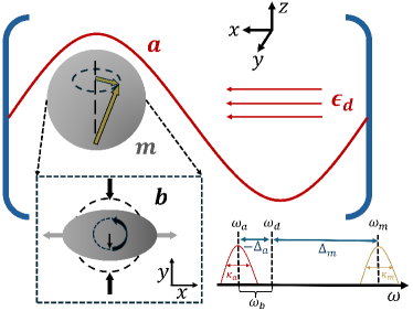
Consider a hybrid cavity magnomechanical system as shown in Fig. 1, where a YIG sphere is inserted into a three-dimensional microwave cavity. The system is constituted by the microwave-mode photons, the magnons provided by the YIG sphere, and the vibrational modes (phonons) of the sphere. The magnons are coupled to photons via the Zeeman interaction and to phonons by the magnetostrictive interaction. The hybrid system has been experimentally realized in recent works [14, 15, 16]. The full system Hamiltonian thus reads ()
| (1) | ||||
where , , and are the annihilation (creation) operators of the photon mode, the magnon of the ground Kittel mode [1], and the phonon mode with transition frequencies , , and , respectively. The magnon-mode frequency is determined by , where is the gyromagnetic ratio and is the external bias magnetic field. Thus, it can be appropriately tuned by the external magnetic field. is the nonlinear coefficient for the Kerr effect due to the ensued magnetocrystalline anisotropy, which can be either positive or negative by adjusting the crystallographic axis of the YIG sphere along the bias magnetic field and is inversely proportional to the volume of the YIG sphere. The Kerr effect cannot be neglected when the magnon excitation number is sufficiently large [15, 58, 8, 3]. is the photon-magnon coupling strength, entering into the strong-coupling regime. The single-magnon magnomechanical coupling strength is typically small, considering the large frequency mismatch between the magnon and the phonon modes, yet it can be compensated by a strong drive. The last term in Eq. (1) describes the external driving of the photon mode, where is the Rabi frequency and is the driving frequency.
The magnon mode under strong driving is assumed to have a large expectation value , which allows us to linearize the system dynamics. Following the standard linearization approach [13, 18], the full system Hamiltonian turns out to be
| (2) | ||||
where is the modified magnon detuning, and is the driving-enhanced Kerr parameter. is the squeezing parameter induced by the linearization of the Kerr effects and . for simplicity, is the driving-enhanced magnomechanical coupling strength. is a phase associated with . The details can be found in Appendix A.
At the large detuning regime, i.e., , and under the near-resonant condition , we can extract an effective Hamiltonian describing the photon-phonon squeezing by perturbative theory [56, 59]. The effective Hamiltonian is found to be
| (3) |
where the effective coupling strength is
| (4) |
and the energy shift is
| (5) |
The details can be found in Appendix B. The phase specifies the squeezing quadrature operator but does not affect the squeezing level. Therefore, we set in the following for simplicity and with no loss of generality. The corresponding squeezing operators can be written as
| (6) |
where . When the initial state is a vacuum state, its variance turns into under the time-evolution of Hamiltonian (3) [35, 43]. Obviously, the quadrature operator is squeezed, i.e., , when .
III The application range of the effective Hamiltonian
In this section, we check the applicability range of the effective Hamiltonian in Eq. (3) in terms of the coupling strengths and squeezing parameters. In previous works [56, 26], diagonalizing the full system Hamiltonian in a truncated finite-dimensional Hilbert space is employed to confirm the effective Hamiltonian constructed by virtual transitions. It is essential to observe a desired avoided level crossing between two eigenstates in the eigenenergies diagram, and the energy splitting at the avoided level crossing point precisely equals twice the effective coupling strength. However, the two-mode squeezing effective Hamiltonian (3) is not conserved in the excitation number, as shown by the non-commutativity with the excitation-number operator. Thus, the effective Hamiltonian (3) cannot be rigorously diagonalized within an appropriate truncated Hilbert space. Additionally, an explicit avoided-level crossing between two eigenstates does not appear for the two-mode squeezing Hamiltonian. Consequently, we propose a distinct method to validate the two-mode squeezing Hamiltonian in Eq. (3).
Under the evolution of the full system Hamiltonian in Eq. (2), the time-evolved quadrature operators in the Heisenberg picture can be written as
| (7) |
where is the vector of quadrature operators, and . represents the Liouvillian superoperator,
| (8) |
where and . The Heisenberg equation in Eq. (7) can be regarded as a discrete Schrödinger equation, where is conceptualized as an effective operator wave function [60]. The superoperator then can be analogously regarded as the full system Hamiltonian, and its diagonalization values are the system’s eigenvalues.
We now analyze the distinct phenomenon observed in the energy diagram of the Liouvillian superoperator at two-mode squeezing. Rotating the effective Hamiltonian (3) with into the lab frame, it becomes
| (9) |
The corresponding Heisenberg equation is
| (10) |
where . Four eigenvalues of the Liouvbilian superoperator can be derived as
| (11) | ||||
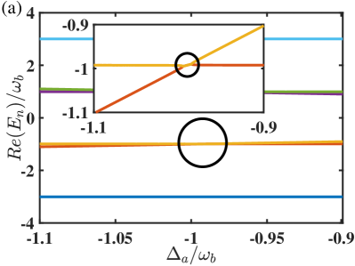
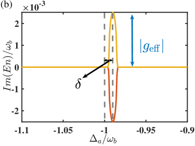
The real parts of the eigenvalues () converge, while the imaginary parts split as the detuning gradually approaches . Until , the real parts of () become identical, while the imaginary parts reach their extreme values of . Then, in the energy-level diagram of the whole superoperator as a function of , one can demonstrate the two-mode squeezing interaction through the level attractions of the real parts and the maximal splittings of the imaginary parts.
We plot the energy levels (all six real and two relevant imaginary parts) in Figs. 2(a) and 2(b), where the eigenvalues are obtained by the standard numerical diagonalization on the whole superoperator in Eq. (8). Figure 2(a) shows the real parts of all six eigenvalues. The light-blue and dark-blue lines describe the energies of the magnon and are not relevant to photon-phonon squeezing. For the other four eigenvalues, two level attractions appear simultaneously as the detuning frequency of photon approaches (but does not exactly equal) the opposite frequency of phonon . This level attraction is highlighted by a dark circle, and the inset further emphasizes it. The imaginary parts of the two relevant eigenvalues (red and orange lines) are illustrated in Fig. 2(b). As the real parts of the two eigenvalues gradually converge, their imaginary parts progressively increase, reaching a maximum absolute value at . The shift is induced by the mutual interaction between the photon (phonon) and the magnon.
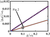
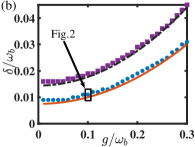
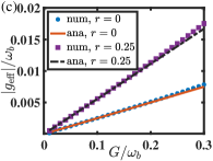
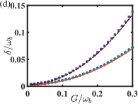
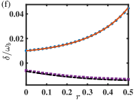
The maximal splitting of the imaginary parts of the two eigenvalues [see Fig. 2(b)] is presented in Figs. 3(a) and 3(c) as a function of the original coupling strengths and in Eq. (2), respectively. The analytical result in Eq. (4) is compared to the numerical simulation over the superoperator in Eq. (8). Blue dots and purple squares represent the numerical results at squeezing parameters and , respectively. The red solid and black dashed lines are the analytical results at and , respectively. In Fig. 3(a), the analytical do match well with their numerical results for the coupling strength , regardless of whether is or . The valid range has entered the ultrastrong coupling regime, [61]. The value distinguished by the black box corresponds to Fig. 2(b). In Fig. 3(c), is valid at the range of when . As increases to , the valid range reduces to . Similarly, the energy shift in Eq. (5) can also be justified by Figs. 3(b) and 3(d). In Fig. 3(b), the analytical shows a slight deviation from the numerical results, but this deviation gradually decreases as and increase. In Fig. 3(d), it is found that the energy shift is valid at , whatever the parameter is or .
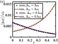
Similar results about and are plotted as a function of the squeezing parameter in Figs. 3(e) and (f), respectively. It is evident that both the analytical results for and match well with the numerical results at . The effective coupling is significantly amplified as increases, which can improve the photon-phonon squeezing level discussed later. However, at , there exists a slight distinction between the numerical and analytical results for both or . This distinction is mainly attributed to the constraint of the parameter setting, which yields that the detuning between magnon and phonon, , is not sufficiently larger than the coupling strengths. Furthermore, decreases as increases, leading to a low two-mode squeezing level.
IV Photon-phonon squeezing
Using the effective Hamiltonian in Eq. (3), one can generate naturally and directly the photon-phonon TMSS. In this section, we take the open-quantum-system framework to discuss the dynamics of TMSS generation and explain why the asymptotic two-mode squeezing can be obtained even in an unstable dynamical evolution. Under the standard assumptions, i.e., Markovian approximation and structure-free environment at zero temperature, the dynamics of the quantum system are governed by the quantum Langevin equation (QLE), written in a matrix form
| (12) |
where is the same as Eq. (10). The transition matrix is
| (13) |
where and are the decay rates of the modes and , respectively. is the vector of Gaussian noise operators, and . and are characterized by their covariance functions, and , where is the mean population of mode at the thermal equilibrium state.
The input zero-mean quantum Gaussian noises yield the quantum state as a zero-mean Gaussian state, which can be completely characterized by a covariance matrix (CM) . By virtue of the QLE in Eq (12), the dynamics of the CM satisfies
| (14) |
The elements of are defined as
| (15) |
where is the -term of and . is the diffusion matrix, which is defined through . In the stable condition, the CM is invariant under time evolution, i.e, in Eq. (14), which requires .
Assume the photon and phonon are both in vacuum states initially, which can be realized by precooling them to their respective ground states [62]. Then the initial CM can be written as , is an identity matrix with four dimensions. Under this initial condition, the non-zero matrix elements in can be solved as
| (16) | ||||
and . The parameters are defined as
| (17) | ||||
And
| (18) | ||||
which are also the solutions of the matrix elements , , and in the stable regime, respectively, obtained by setting in Eq. (14). These stable CM elements are the asymptotic values as .
With the CM definition in Eq. (15) and its solution in Eq. (16), the variance of the quadrature operator in Eq. (6) can be derived as
| (19) | ||||
where
| (20) |
In the stable regime, , one can demonstrate that the exponent factor in Eq. (19) is negative through the definition of in Eq. (17). That leads to , consistent with the result obtained by . When the photon decay rate is larger than the phonon decay rate, i.e., , the minimal value of can be obtained as
| (21) |
at . Even at the zero temperature, , the minimum . The value corresponds to the upper bound of the squeezing level, dB, under the stable condition. The squeezing level in the decibel unit is defined by [63], where is the standard fluctuation in the zero-point level. The decay rates satisfy in the recent cavity magnomechanical system [14], resulting in even when . It implies that cannot be squeezed under stable conditions in this specific experimental platform.
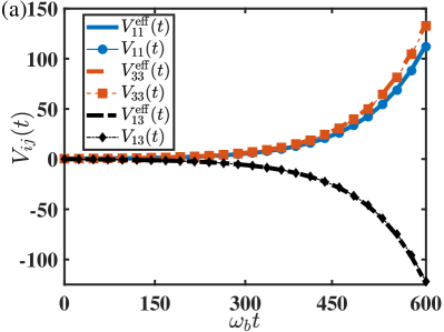
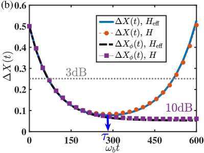
In the unstable regime, , all the CM elements , , and in Eq. (16) exhibit exponential divergence due to the exponential factor . These are clearly illustrated by their respective numerical results, shown by a blue-solid line, a red-dashed line, and a black dash-dotted line in Fig. 4(a). The corresponding variance in Eq. (19) is depicted by a blue solid line in Fig. 4(b). One can observe that it initially decreases until it reaches its minimum value , where the moment can be analytically determined by setting the derivation . After reaching its minimum, increases exponentially, and .
However, both the CM and the variance instabilities do not imply nonstationary TMSS. To find a stationary TMSS with a higher squeezing level, we define a general two-mode squeezing operator , where is an angle to optimize. With the CM elements (16), its variance can be described as
| (22) | ||||
where and , are constants in Eq. (18).
From Eq. (22), one can find that the exponential divergence term of can be canceled at an optimized angle , i.e., the angle satisfies
| (23) |
Specifically, at . Under this optimized angle, turns into
| (24) |
It is evident that , corresponding to the standard fluctuation in the zero-point level [63]. The condition signifies the occurrence of two-mode squeezing during the evolution [63]. The value of quantifies the level of the squeezing, a smaller yielding a stronger squeezing. Equation (24) also shows an asymptotic stationary squeezing over a long evolution, i.e.,
| (25) |
Given the definition of in Eq. (17), it follows that decreases as well as the two-mode squeezing enhances as increases.
It is a natural result of the system’s evolution under the two-mode squeezing Hamiltonian (3) in the open quantum system framework. The two-mode squeezing interaction generates the photon-phonon squeezing, gradually increasing the squeezing level over time. In contrast, Markovian noises reduce the squeezing as time progresses. Both factors constitute a competitive mechanism in the open-quantum-system framework, leading to an asymptotic stationary photon-phonon squeezing with an optimized squeezing operator.
In Fig. 4 (b), we plot using the effective Hamiltonian by blue dash-dotted line. After a long time evolution , it tends to stabilize a certain value of , and the corresponding squeezing level is about dB below vacuum fluctuation, which is larger than the upper bound dB in the stable dynamic condition.

We also simulate the logarithmic negativity (LN) to quantify the photon-phonon squeezing (EPR entanglement) [64, 65, 66], which is defined as
| (26) |
, with , , and being the blocks of , and . Then, the time-dependent LN can be derived as
| (27) |
where and . In the unstable dynamical regime , using the solutions in Eq. (16), one can demonstrate that when . With the Taylor expansion up to the first order of , one can finally obtain the LN at infinity
| (28) |
When asymptotic stationary two-mode squeezing emerges during unstable dynamics, as indicated by , asymptotic stationary bipartite entanglement between the photon and phonon also arises. The LN increases with the value of decreases, indicating that stronger two-mode squeezing corresponds to greater entanglement.
The above results obtained by the effective Hamiltonian in Eq. (3) can be further confirmed by the whole system’s dynamics. Similar as Eq. (14), using the full system Hamiltonian in Eq. (2), the dynamics of the whole system CM is determined by
| (29) |
The elements of are defined as
| (30) |
where is shown in Eq. (7). The transition matrix , where is the superoperator in Eq. (8) and . The magnon decay rate is exponentially enlarged due to the Kerr effect, i.e., [67]. is the matrix of noises covariance. Then, the dynamics of and can be obtained by numerically calculating the CM ,
| (31) | ||||
The initial condition is , and is a six-dimensional identity matrix.
Numerical results are shown in Figs. 4(a) and (b). All of the matrix elements in Fig. 4(a), (blue solid line with circles), (red dashed line with squares), and (black dash-dotted line with diamonds), along with the variances in Fig. 4(b), (red dashed line with circles) and (purple dotted line with squares) obtained using Eq. (29) do match well with the corresponding results via the effective Hamiltonian (3).
We also numerically analyze the asymptotic stationary LN, , using the whole system’s dynamics to evaluate our protocol. For the whole system, the is defined by replacing the in Eq. (26) with in Eq. (29). Besides, we approximate by evaluating the value after a sufficient long time, specifically , where is the moment when in Eq. (19) reaches its minimum, as shown in Fig. 4 (b).
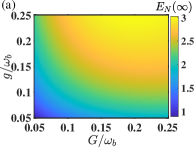
In Fig. 5(a), we illustrate the in the parameter space of coupling strengths and . One can observe that a high entanglement LN can be obtained when the coupling strengths and are increased. The LN is greater than for . In Fig. 5(b), we present in the parameter space defined by magnon detuning and the squeezing parameter . A low entanglement regime around is observed, and the low-region enhances with increasing , which is attributed to the invalidity of the effective Hamiltonian (3) constructed in perturbation condition. In the region where , the effective coupling strength decreases as increases [see Fig. 3(e)], which leads to a reduction in LN with increasing . In contrast, when , the effective coupling increases as increases, leading consequently to a enhancement of the LN with increasing . However, under the constraint of the large detuning condition, i.e., , an even larger does not always yield better results. A larger allows a broader range of to achieve a high LN. An optimal parameter space exists at . From these findings, we conclude that our protocol significantly enhances the asymptotic stationary LN, , from the previously reported values of approximately [18]. It can also exceed the maximum theoretical limit at the stable dynamic condition, i.e., [39].
V Discussion and Conclusion
Our protocol is primarily centered on the cavity magnomechanical system, focusing on constructing the magnon-assisted photon-phonon squeezing. In recent experiments [14, 15, 16], the coupling strength between photon and magnon, MHz, is about , where the phonon frequency MHz. The single-excitation magnon-phonon coupling is related to the volume of the YIG sphere and the biased magnetic field directions. For a YIG sphere with a diameter m, the coupling strength is approximately Hz [14]. The Rabi frequency of driving is defined as [15, 16], where is the cavity decay rate associated with the driving point, and represent the power and frequency of the microwave drive, respectively. In recent experiments [15], MHz and dBm (mW). They give rise a Rabi frequency Hz, corresponding to . The enhanced coupling between magnon and phonon is given by . Consequently, the effective coupling strength satisfies . These values are consistent with the parameters used in Figs. 2 and 3. The magnon Kerr effect can be enhanced by reducing the volume of the YIG sphere [8, 68, 58]. For specifical parameters nHz, , and , the squeezing parameter roughly equals . The decay rates of phonon and photon modes are and , respectively. Thus, the cooperativity . The unstable dynamical regime in our protocol, characterized by , can be successfully realized. Besides, the magnon decay rate, , is challenging to reduce further due to intrinsic damping [2]. However, its impact is insignificant as the magnon primarily serves as an interface. At a low temperature of , the thermal occupations of photon, magnon, and phonon are respective , , and , consistent with the parameters used in Figs. 4 and 5.
In summary, we have presented a protocol for generating photon-phonon squeezing in the cavity magnomechanics, where the magnon in the YIG sphere is coupled to both microwave photons and the mechanical vibration modes in the same sphere. Our protocol offers significant advantages in terms of controllability within the system, and the Kerr effect of magnon can further enhance the squeezing level in a proper regime. This magnon-assisted protocol relies on the effective two-mode squeezing Hamiltonian for coupling photons and phonons. We apply an interesting method by diagonalizing the whole system’s Liouvillian superoperator to numerically confirm the validity of the effective Hamiltonian, which is beneficial to more physics with nonconservative excitations. In the open-quantum-system framework, we derive the process for generating TMSS with the effective Hamiltonian. Our analysis demonstrates that the asymptotic stationary TMSS with high squeezing levels can be achieved even in unstable dynamics. Our work provides an important implementation of TMSS generation in a solid system under realistic noises. It extends the application of cavity magnomechanics as a promising hybrid platform for quantum information processing.
In addition to the cavity magnomechanical system, our protocol can be extended to other quantum systems. For instance, we can utilize a mechanical interface to realize the microwave-optical photon squeezed state [69, 70] or create the photon-magnon squeezed state [57]. Our scheme presents an extendable framework to create TMSS, which will be widely applied in quantum information processing and quantum metrology using bosonic systems.
Acknowledgments
We acknowledge financial support from the National Science Foundation of China (Grant No. 12404405) and the Science Foundation of Hebei Normal University of China (Grant No. L2024B10).
Appendix A System linearized Hamiltonian
This appendix contributes to deriving the linearized Hamiltonian in Eq. (2). With respect to the transformation , the original Hamiltonian in Eq. (1) turns out to be
| (32) |
where and . Due to the Heisenberg-Langevin equation, the time evolution of the system operators satisfies
| (33) | ||||
where , and are the input noise operators for the cavity photon, magnon, and phonon modes, respectively, which are characterized by the covariance functions: and , under the Markovian approximation. is the mean population of mode at the thermal equilibrium state. , , and are the decay rates of the modes , and , respectively.
Under the condition that the photon mode under strong driving, it has a large amplitude at its steady state. Due to the strong photon-magnon dipole-dipole interaction, the magnon mode also has a large amplitude . This allows us to linearize the system’s dynamics around the steady state values by writing the operators , is the operator describing the small quantum fluctuation. The steady values satisfy
| (34) | ||||
Then we have
| (35) | ||||
When and both and are significantly small, the steady magnitude of magnon mode approximately equals to .
By substituting the steady values in Eq. (35) into the equations in Eq. (33) and ignoring all the high-order terms of fluctuations, the Heisenberg-Langevin equations describing the fluctuation operators can be written as
| (36) | ||||
The corresponding effective linearized Hamiltonian can be described as
| (37) |
where , , , and . We apply the convention in the following content for simplicity.
In the rotating frame with the unitary transformation , the linearized Hamiltonian in Eq. (37) transforms into
| (38) | ||||
Setting and , the quadratic terms about and can be canceled. Then the Hamiltonian in Eq. (38) can be reduced into
| (39) | ||||
where . The effective magnon coupling strength can be written as due to . It is the linearized Hamiltonian (2) in the main text. For simplicity, we apply the conventions and in the main manuscript and the following content.
Appendix B Effective Hamiltonian for photon-phonon squeezing
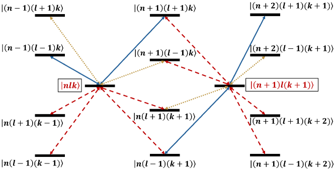
To realize the photon-phonon squeezing assisted by the magnon mode via the linearized Hamiltonian in Eq. (39), generally one can extract an effective transition from the near-degenerate subspaces based on the perturbation theory concerning the coupling strengths and . When the photon detuning frequency is almost opposite the phonon frequency , and both of them are far resonant from the detuning , i.e., and , it is found that the tensor-product state is near degenerate with . Here the subscripts respectively represent the photon, magnon, and phonon modes, and indicate their individual Fock states. To the second order, the effective coupling strength or the energy shift between any eigenstates and of the unperturbed Hamiltonian in Eq. (39) is given by [56, 59, 71]
| (40) |
where is the eigenenergy of state , provided the interaction Hamiltonian is regarded as a perturbation to .
A good approximation of the effective Hamiltonian describing the transition between arbitrary base pair and can be analytically obtained using the preceding second-order perturbation theory. It can be expressed in the form
| (41) |
where and are the energy shifts due to the coupling for the states and , respectively. is the effective coupling strength. These are three coefficients to be determined in this ansatz. We here omit the common unperturbed eigenenergy of two bases .
We first consider the energy shift for the state . Summarizing all the eight paths from to through an intermediate state, as shown in Fig. 6, one can obtain the second-order energy correction for the according to Eq. (40)
| (42) |
And in the same way, the energy shift for the state is found to be
| (43) |
An exact resonance between arbitrary and requires that the first two terms in Eq. (41) constitute the identity operator in the relevant subspace. Thus, . Assuming the distance between and is , one can have
| (44) | ||||
where represents all the higher orders of from the first order in Taylor expansion. Then is consistently solved as up to the second-order correction. Note , so that up to the second order of the coupling strengths and , we have
| (45) |
via . Interestingly, is a Fock-state-independent coefficient in comparison to both and .
References
- Rameshti et al. [2022] B. Z. Rameshti, S. V. Kusminskiy, J. A. Haigh, K. Usami, D. Lachance-Quirion, Y. Nakamura, C.-M. Hu, H. X. Tang, G. E. Bauer, and Y. M. Blanter, Cavity magnonics, Phys. Rep. 979, 1 (2022).
- Yuan et al. [2022] H. Yuan, Y. Cao, A. Kamra, R. A. Duine, and P. Yan, Quantum magnonics: When magnon spintronics meets quantum information science, Phys. Rep. 965, 1 (2022).
- Wang et al. [2018] Y.-P. Wang, G.-Q. Zhang, D. Zhang, T.-F. Li, C.-M. Hu, and J. Q. You, Bistability of cavity magnon polaritons, Phys. Rev. Lett. 120, 057202 (2018).
- Tabuchi et al. [2014] Y. Tabuchi, S. Ishino, T. Ishikawa, R. Yamazaki, K. Usami, and Y. Nakamura, Hybridizing ferromagnetic magnons and microwave photons in the quantum limit, Phys. Rev. Lett. 113, 083603 (2014).
- Shen et al. [2021] R.-C. Shen, Y.-P. Wang, J. Li, S.-Y. Zhu, G. S. Agarwal, and J. Q. You, Long-time memory and ternary logic gate using a multistable cavity magnonic system, Phys. Rev. Lett. 127, 183202 (2021).
- Tabuchi et al. [2015] Y. Tabuchi, S. Ishino, A. Noguchi, T. Ishikawa, R. Yamazaki, K. Usami, and Y. Nakamura, Coherent coupling between a ferromagnetic magnon and a superconducting qubit, Science 349, 405 (2015).
- Xu et al. [2023] D. Xu, X.-K. Gu, H.-K. Li, Y.-C. Weng, Y.-P. Wang, J. Li, H. Wang, S.-Y. Zhu, and J. Q. You, Quantum control of a single magnon in a macroscopic spin system, Phys. Rev. Lett. 130, 193603 (2023).
- Wang et al. [2016] Y.-P. Wang, G.-Q. Zhang, D. Zhang, X.-Q. Luo, W. Xiong, S.-P. Wang, T.-F. Li, C.-M. Hu, and J. Q. You, Magnon kerr effect in a strongly coupled cavity-magnon system, Phys. Rev. B 94, 224410 (2016).
- Ladd et al. [2010] T. D. Ladd, F. Jelezko, R. Laflamme, Y. Nakamura, C. Monroe, and J. L. O’Brien, Quantum computers, Nature (London) 464, 45 (2010).
- Reiserer and Rempe [2015] A. Reiserer and G. Rempe, Cavity-based quantum networks with single atoms and optical photons, Rev. Mod. Phys. 87, 1379 (2015).
- Degen et al. [2017] C. L. Degen, F. Reinhard, and P. Cappellaro, Quantum sensing, Rev. Mod. Phys. 89, 035002 (2017).
- Blais et al. [2021] A. Blais, A. L. Grimsmo, S. M. Girvin, and A. Wallraff, Circuit quantum electrodynamics, Rev. Mod. Phys. 93, 025005 (2021).
- Aspelmeyer et al. [2014] M. Aspelmeyer, T. J. Kippenberg, and F. Marquardt, Cavity optomechanics, Rev. Mod. Phys. 86, 1391 (2014).
- Zhang et al. [2016] X. Zhang, C.-L. Zou, L. Jiang, and H. Tang, Cavity magnonmechanics, Sci. Adv. 2, e1501286 (2016).
- Shen et al. [2022] R.-C. Shen, J. Li, Z.-Y. Fan, Y.-P. Wang, and J. Q. You, Mechanical bistability in kerr-modified cavity magnomechanics, Phys. Rev. Lett. 129, 123601 (2022).
- Potts et al. [2021] C. A. Potts, E. Varga, V. A. S. V. Bittencourt, S. V. Kusminskiy, and J. P. Davis, Dynamical backaction magnomechanics, Phys. Rev. X 11, 031053 (2021).
- Zuo et al. [2024] X. Zuo, Z.-Y. Fan, H. Qian, M.-S. Ding, H. Tan, H. Xiong, and J. Li, Cavity magnomechanics: from classical to quantum, New J. Phys. 26, 031201 (2024).
- Li et al. [2018] J. Li, S.-Y. Zhu, and G. S. Agarwal, Magnon-photon-phonon entanglement in cavity magnomechanics, Phys. Rev. Lett. 121, 203601 (2018).
- Yu et al. [2020] M. Yu, H. Shen, and J. Li, Magnetostrictively induced stationary entanglement between two microwave fields, Phys. Rev. Lett. 124, 213604 (2020).
- Chen et al. [2021] Y.-T. Chen, L. Du, Y. Zhang, and J.-H. Wu, Perfect transfer of enhanced entanglement and asymmetric steering in a cavity-magnomechanical system, Phys. Rev. A 103, 053712 (2021).
- Tan [2019] H. Tan, Genuine photon-magnon-phonon einstein-podolsky-rosen steerable nonlocality in a continuously-monitored cavity magnomechanical system, Phys. Rev. Res. 1, 033161 (2019).
- Li et al. [2019] J. Li, S.-Y. Zhu, and G. S. Agarwal, Squeezed states of magnons and phonons in cavity magnomechanics, Phys. Rev. A 99, 021801 (2019).
- Li et al. [2023] J. Li, Y.-P. Wang, J.-Q. You, and S.-Y. Zhu, Squeezing microwaves by magnetostriction, Natl. Sci. Rev. 10, nwac247 (2023).
- Qian et al. [2024] H. Qian, X. Zuo, Z.-Y. Fan, J. Cheng, and J. Li, Strong squeezing of microwave output fields via reservoir-engineered cavity magnomechanics, Phys. Rev. A 109, 013704 (2024).
- Sarma et al. [2021] B. Sarma, T. Busch, and J. Twamley, Cavity magnomechanical storage and retrieval of quantum states, New J. Phys. 23, 043041 (2021).
- Qi and Jing [2021] S.-f. Qi and J. Jing, Magnon-assisted photon-phonon conversion in the presence of structured environments, Phys. Rev. A 103, 043704 (2021).
- Qi and Jing [2022] S.-f. Qi and J. Jing, Accelerated adiabatic passage in cavity magnomechanics, Phys. Rev. A 105, 053710 (2022).
- Lloyd and Braunstein [1999] S. Lloyd and S. L. Braunstein, Quantum computation over continuous variables, Phys. Rev. Lett. 82, 1784 (1999).
- Braunstein and van Loock [2005] S. L. Braunstein and P. van Loock, Quantum information with continuous variables, Rev. Mod. Phys. 77, 513 (2005).
- Furusawa et al. [1998] A. Furusawa, J. L. Sørensen, S. L. Braunstein, C. A. Fuchs, H. J. Kimble, and E. S. Polzil, Unconditional quantum teleportation, Science 282, 706 (1998).
- Giovannetti et al. [2011] V. Giovannetti, S. Lloyd, and L. Maccone, Advanced in quantum metrology, Nat. Photonics 5, 222 (2011).
- Masada et al. [2015] G. Masada, K. Miyata, A. Politi, T. Hashimoto, J. L.O’Brien, and A. Furusawa, Continuous-variable entanglement on a chip, Nat. Photonics 9, 316 (2015).
- Villar et al. [2005] A. S. Villar, L. S. Cruz, K. N. Cassemiro, M. Martinelli, and P. Nussenzveig, Generation of bright two-color continuous variable entanglement, Phys. Rev. Lett. 95, 243603 (2005).
- Heidmann et al. [1987] A. Heidmann, R. J. Horowicz, S. Reynaud, E. Giacobino, C. Fabre, and G. Camy, Observation of quantum noise reduction on twin laser beams, Phys. Rev. Lett. 59, 2555 (1987).
- Sahu et al. [2023] R. Sahu, L. Qiu, W. Hease, G. Arnold, Y. Minoguchi, P. Rabl, and J. Fink, Entangling microwaves with light, Science 380, 718 (2023).
- Reid and Drummond [1988] M. D. Reid and P. D. Drummond, Quantum correlations of phase in nondegenerate parametric oscillation, Phys. Rev. Lett. 60, 2731 (1988).
- Ou et al. [1992] Z. Y. Ou, S. F. Pereira, H. J. Kimble, and K. C. Peng, Realization of the einstein-podolsky-rosen paradox for continuous variables, Phys. Rev. Lett. 68, 3663 (1992).
- Qurjoumtsev et al. [2011] A. Qurjoumtsev, A. Kubanek, M. Koch, C. Sames, P. W. H. Pinkse, G. Rempe, and K. Murr, Observation of squeezed light from one atom excited with two photons, Nature (London) 474, 623 (2011).
- Wang and Clerk [2013] Y.-D. Wang and A. A. Clerk, Reservoir-engineered entanglement in optomechanical systems, Phys. Rev. Lett. 110, 253601 (2013).
- Tian [2013] L. Tian, Robust photon entanglement via quantum interference in optomechanical interfaces, Phys. Rev. Lett. 110, 233602 (2013).
- Li et al. [2015] Z. Li, S.-l. Ma, and F.-l. Li, Generation of broadband two-mode squeezed light in cascaded double-cavity optomechanical systems, Phys. Rev. A 92, 023856 (2015).
- Tan et al. [2013] H. Tan, G. Li, and P. Meystre, Dissipation-driven two-mode mechanical squeezed states in optomechanical systems, Phys. Rev. A 87, 033829 (2013).
- Pontin et al. [2016] A. Pontin, M. Bonaldi, A. Borrielli, L. Marconi, F. Marino, G. Pandraud, G. A. Prodi, P. M. Sarro, E. Serra, and F. Marin, Dynamical two-mode squeezing of thermal fluctuations in a cavity optomechanical system, Phys. Rev. Lett. 116, 103601 (2016).
- Julsgaard et al. [2001] B. Julsgaard, A. Kozhekin, and E. S. Polzik, Experimental long-lived entanglement of two macroscopic objects, Nature (London) 413, 400 (2001).
- Gross et al. [2011] C. Gross, H. Strobel, E. Nicklas, T. Zibold, N. Bar-Gill, G. Kurizki, and M. K. Oberthaler, Atomic homodyne detection of continuous-variable entangled twin-atom states, Nature (London) 480, 219 (2011).
- Bookjans et al. [2011] E. M. Bookjans, C. D. Hamley, and M. S. Chapman, Strong quantum spin correlations observed in atomic spin mixing, Phys. Rev. Lett. 107, 210406 (2011).
- Qu et al. [2020] A. Qu, B. Evrard, J. Dalibard, and F. Gerbier, Probing spin correlations in a bose-einstein condensate near the single-atom level, Phys. Rev. Lett. 125, 033401 (2020).
- Kim et al. [2021] K. Kim, J. Hur, S. Huh, S. Choi, and J.-y. Choi, Emission of spin-correlated matter-wave jets from spinor bose-einstein condensates, Phys. Rev. Lett. 127, 043401 (2021).
- Sundar et al. [2023] B. Sundar, D. Barberena, A. P. n. Orioli, A. Chu, J. K. Thompson, A. M. Rey, and R. J. Lewis-Swan, Bosonic pair production and squeezing for optical phase measurements in long-lived dipoles coupled to a cavity, Phys. Rev. Lett. 130, 113202 (2023).
- Bilitewski and Rey [2023] T. Bilitewski and A. M. Rey, Manipulating growth and propagation of correlations in dipolar multilayers: From pair production to bosonic kitaev models, Phys. Rev. Lett. 131, 053001 (2023).
- Duha and Bilitewski [2024] A. Duha and T. Bilitewski, Two-mode squeezing in floquet-engineered power-law interacting spin models, Phys. Rev. A 109, L061304 (2024).
- Mamaev et al. [2024] M. Mamaev, M. Koppenhöfer, A. Pocklington, and A. A.Clerk, Non-gaussian generalized two-mode squeezing: applications to two-ensemble spin squeezing and beyond, arxiv: 2407, 00721v1 (2024).
- Römling and Kamra [2024] A.-L. E. Römling and A. Kamra, Quantum sensing of antiferromagnetic magnon two-mode squeezed vacuum, Phys. Rev. B 109, 174410 (2024).
- Esposito et al. [2022] M. Esposito, A. Ranadive, L. Planat, S. Leger, D. Fraudet, V. Jouanny, O. Buisson, W. Guichard, C. Naud, J. Aumentado, F. Lecocq, and N. Roch, Observation of two-mode squeezing in a traveling wave parametric amplifier, Phys. Rev. Lett. 128, 153603 (2022).
- Andersson et al. [2022] G. Andersson, S. W. Jolin, M. Scigliuzzo, R. Borgani, M. O. Tholén, J. Rivera Hernández, V. Shumeiko, D. B. Haviland, and P. Delsing, Squeezing and multimode entanglement of surface acoustic wave phonons, PRX Quantum 3, 010312 (2022).
- Garziano et al. [2016] L. Garziano, V. Macrì, R. Stassi, O. Di Stefano, F. Nori, and S. Savasta, One photon can simultaneously excite two or more atoms, Phys. Rev. Lett. 117, 043601 (2016).
- Fan et al. [2023] Z.-Y. Fan, L. Qiu, S. Gröblacher, and J. Li, Microwave-optics entanglement via cavity optomagnomechanics, Laser Photonics Rev. 17, 2200866 (2023).
- Xiong et al. [2022] W. Xiong, M. Tian, G.-Q. Zhang, and J. Q. You, Strong long-range spin-spin coupling via a kerr magnon interface, Phys. Rev. B 105, 245310 (2022).
- Kockum et al. [2017] A. F. Kockum, A. Miranowicz, V. Macrì, S. Savasta, and F. Nori, Deterministic quantum nonlinear optics with single atoms and virtual photons, Phys. Rev. A 95, 063849 (2017).
- Chu et al. [2024] Y. Chu, X. Li, and J. Cai, Quantum delocalization on correlation landscape: The key to exponentially fast multipartite entanglement generation, Phys. Rev. Lett. 133, 110201 (2024).
- Forn-Díaz et al. [2019] P. Forn-Díaz, L. Lamata, E. Rico, J. Kono, and E. Solano, Ultrastrong coupling regimes of light-matter interaction, Rev. Mod. Phys. 91, 025005 (2019).
- Ding et al. [2020] M.-S. Ding, L. Zheng, and C. Li, Ground-state cooling of a magnomechanical resonator induced by magnetic damping, J. Opt. Soc. Am. B 37, 627 (2020).
- Zhang et al. [2019a] R. Zhang, Y. Fang, Y.-Y. Wang, S. Chesi, and Y.-D. Wang, Strong mechanical squeezing in an unresolved-sideband optomechanical system, Phys. Rev. A 99, 043805 (2019a).
- Vidal and Werner [2002] G. Vidal and R. F. Werner, Computable measure of entanglement, Phys. Rev. A 65, 032314 (2002).
- Adesso and Illuminati [2007] G. Adesso and F. Illuminati, Entanglement in continuous-variable systems: recent advances and current perspectives, J. Phys. A 40, 7821 (2007).
- Plenio [2005] M. B. Plenio, Logarithmic negativity: A full entanglement monotone that is not convex, Phys. Rev. Lett. 95, 090503 (2005).
- Hei et al. [2023] X.-L. Hei, P.-B. Li, X.-F. Pan, and F. Nori, Enhanced tripartite interactions in spin-magnon-mechanical hybrid systems, Phys. Rev. Lett. 130, 073602 (2023).
- Zhang et al. [2019b] G.-Q. Zhang, Y.-P. Wang, and J. Q. You, Theory of the magnon kerr effect in cavity magnonics, Sci. China Phys. Mech. Astron. 62, 987511 (2019b).
- Barzanjeh et al. [2015] S. Barzanjeh, S. Guha, C. Weedbrook, D. Vitali, J. H. Shapiro, and S. Pirandola, Microwave quantum illumination, Phys. Rev. Lett. 114, 080503 (2015).
- Wu et al. [2020] M. Wu, E. Zeuthen, K. C. Balram, and K. Srinivasan, Microwave-to-optical transduction using a mechanical supermode for coupling piezoelectric and optomechanical resonators, Phys. Rev. Appl. 13, 014027 (2020).
- Shao et al. [2017] W. Shao, C. Wu, and X.-L. Feng, Generalized james’ effective hamiltonian method, Phys. Rev. A 95, 032124 (2017).