This paper was converted on www.awesomepapers.org from LaTeX by an anonymous user.
Want to know more? Visit the Converter page.

Kernel Embedding based Variational Approach for Low-dimensional Approximation of Dynamical Systems

Wenchong Tian 111College of Environmental Science and Engineering, Tongji University, Shanghai 200092, P. R. China, E-mail: [email protected]    Hao Wu 222Correspond Author, School of Mathematical Sciences, Tongji University, Shanghai 200092, P. R. China, E-mail: [email protected]
Abstract

Transfer operators such as Perron-Frobenius or Koopman operator play a key role in modeling and analysis of complex dynamical systems, which allow linear representations of nonlinear dynamics by transforming the original state variables to feature spaces. However, it remains challenging to identify the optimal low-dimensional feature mappings from data. The variational approach for Markov processes (VAMP) provides a comprehensive framework for the evaluation and optimization of feature mappings based on the variational estimation of modeling errors, but it still suffers from a flawed assumption on the transfer operator and therefore sometimes fails to capture the essential structure of system dynamics. In this paper, we develop a powerful alternative to VAMP, called kernel embedding based variational approach for dynamical systems (KVAD). By using the distance measure of functions in the kernel embedding space, KVAD effectively overcomes theoretical and practical limitations of VAMP. In addition, we develop a data-driven KVAD algorithm for seeking the ideal feature mapping within a subspace spanned by given basis functions, and numerical experiments show that the proposed algorithm can significantly improve the modeling accuracy compared to VAMP.

1 Introduction

It has been shown that complex nonlinear processes can be accurately described by linear models in many science and engineering fields, including wireless communications [19, 56], molecular dynamics [54, 4, 55], fluid dynamics [28, 43] and control theory [1], where the linear models can be expressed by a unified formula

𝔼[𝐟(𝐱t+τ)]=𝐊𝔼[𝐟(𝐱t)],\mathbb{E}\left[\mathbf{f}(\mathbf{x}_{t+\tau})\right]=\mathbf{K}^{\top}\mathbb{E}[\mathbf{f}(\mathbf{x}_{t})], (1)

and the expectation operator can be removed for deterministic systems. In such models, the state variable 𝐱\mathbf{x} is tranformed into a feature space by the transformation 𝐟(𝐱)=(f1(𝐱),,fm(𝐱))\mathbf{f}(\mathbf{x})=\left(f_{1}(\mathbf{x}),\ldots,f_{m}(\mathbf{x})\right)^{\top}, and the dynamics with lag time τ\tau is characterized by a linear time-invariant system in the feature space. Then, all the dynamical properties of the system can be quantitatively analyzed after estimating the transition matrix 𝐊\mathbf{K} from data via linear regression. A special case of the linear models is Markov state models [39, 35] for conformational dynamics, which is equivalent to the well-known Ulam’s method [8, 14]. In a Markov state model, the feature mapping 𝐟\mathbf{f} consists of indicator functions of subsets of state and 𝐊=[Kij]\mathbf{K}=[K_{ij}] represents the transition probability from subset ii to subset jj. Besides Markov state models and the Ulam’s method, a large number of similar modeling methods, e.g., dynamic mode decomposition [38, 2, 48, 21], time-lagged independent component analysis (TICA) [30, 34, 41], extended dynamic mode decomposition (EDMD) [50, 16, 40], Markov transition models [52], variational approach of conformation dynamics (VAC) [31, 32, 33], variational Koopman models [54] and their variants based on kernel ebmeddings [15, 16] and tensors [14, 33], are proposed by using different feature mappings.

From the perspective of operator theory, all the models in the form of (1) can be interpreted as algebraic representations of transfer operators of systems, including Frobenius-Perron (FP) operators and Koopman operators, and some of them are universal approximators for nonlinear dynamical systems under the assumption that the dimension of feature space is large enough [20] or the infinite-dimensional kernel mappings are utilized [45]. However, due to the limitation of computational cost and requirements of dynamical analysis, the low-dimensional approximation of transfer operators is still a critical and challenging problem in applications [17].

One common way to solve this problem is to identify the dominant dynamical structures, e.g., metastable states [9, 37], cycles [6] and coherent sets [11], and achieve the corresponding low-dimensional representations via spectral clustering. But this strategy assumes that an accurate high-dimensional model is known a priori, which is often violated especially for large-scale systems.

Another way for deterministic systems is to seek the feature mapping 𝐟\mathbf{f} by minimizing the regression error of (1) under the constraint that the state variable can also be accurately reconstructed from 𝐟\mathbf{f} [23, 24]. Notice that the constraint is necessary, otherwise a trivial but uninformative model with 𝐟(𝐱)1\mathbf{f}(\mathbf{x})\equiv 1 and 𝐊=1\mathbf{K}=1 could be found. Some similar methods are developed for stochastic systems by considering (1) as a conditional generative model, where the parameters of 𝐟\mathbf{f} can be trained based on the likelihood or the other statistical criteria [51, 25]. However, these methods are applicable only if 𝐟\mathbf{f} are non-negative functions and usually involves the intractable probability density estimation.

In recent years, the variational approach has led to great progress for low-dimensional dynamical modeling, which was first proposed for time-reversible processes [31, 32, 27, 54] and extended to non-reversible processes in [53]. In contrast with the other methods, this approach provides a general and unified framework for data-driven model choice, reduction and optimization of dynamical systems based on the presented variational scores related to approximation errors of transfer operators. It can be easily integrated with deep learning to effectively analyze high-dimensional time series in an end-to-end manner [26, 3]. The existing variational principle based methods suffer from two drawbacks: First, it is necessary to assume that the transfer operator is Hilbert-Schimdt (HS) or compact as an operator between two weighted 2\mathcal{L}^{2} spaces so that the maximum values of variational scores exist. But there is no easy way to test the assumption especially when we do not have strong prior knowledge regarding the system. Specifically, it can be proved that the assumption does not hold for most deterministic systems. Second, even for stochastic systems which satisfies the assumption, the common variational scores are possibly sensitive to small modeling variations, which could affect the effectiveness of the variational approach.

In this work, we introduce a kernel embedding based variational approach for dynamical systems (KVAD) using the theory of kernel embedding of functions [44, 46, 47, 45], where the modeling error is measured by using the distance between kernel embeddings of transition densities. The kernel based variational score in KVAD provides a robust and smooth quantification of differences between transfer operators, and is proved to be bounded for general dynamical systems, including deterministic and stochastic systems. Hence, it can effectively overcome the difficulties of existing variational methods, and expands significantly the range of applications. Like the previous variational scores, the kernel based score can also be consistently estimated from trajectory data without solving any intermediate statistical problem. Therefore, we develop a data-driven KVAD algorithm by considering 𝐟\mathbf{f} as a linear superposition of a given set of basis functions. Furthermore, we establish a relationship between KVAD, diffusion maps[5] and the singular components of transfer operators. Finally, the effectiveness the proposed algorithm is demonstrated by numerical experiments.

2 Problem formulation and preliminaries

For a Markovian dynamical system in the state space 𝕄D\mathbb{M}\subset\mathbb{R}^{D} , its dynamics can be completely characterized by the transition density

pτ(𝐱,𝐲)(𝐱t+τ=𝐲|𝐱t=𝐱)p_{\tau}(\mathbf{x},\mathbf{y})\triangleq\mathbb{P}\left(\mathbf{x}_{t+\tau}=\mathbf{y}|\mathbf{x}_{t}=\mathbf{x}\right) (2)

and the time evolution of the system state distribution can be formulated as

pt+τ(𝐲)=(𝒫τpt)(𝐲)pt(𝐱)pτ(𝐱,𝐲)d𝐱,p_{t+\tau}(\mathbf{y})=(\mathcal{P}_{\tau}p_{t})(\mathbf{y})\triangleq\int p_{t}(\mathbf{x})p_{\tau}(\mathbf{x},\mathbf{y})\mathrm{d}\mathbf{x}, (3)

Here 𝐱t\mathbf{x}_{t} denotes the state of the system at time tt and ptp_{t} is the probability density of 𝐱t\mathbf{x}_{t}. The transfer operator 𝒫τ\mathcal{P}_{\tau} is called the Perron-Frobenius (PF) operator333Another commonly used transfer operator for Markovian dynamics is Koopman operator [49], which describes the evolution of observables instead of probability densities, and is the dual of the PF operator. In this paper, we focus only on the PF operator for convenience of analysis., which is a linear but usually infinite-dimensional operator. Notice that the deterministic dynamics in the form of 𝐱t+τ=Θτ(𝐱t)\mathbf{x}_{t+\tau}=\Theta_{\tau}(\mathbf{x}_{t}) is a specific case of the Markovian dynamics, where pτ(𝐱,)=δΘτ(𝐱)()p_{\tau}(\mathbf{x},\cdot)=\delta_{\Theta_{\tau}(\mathbf{x})}(\cdot) is a Dirac function centered at Θτ(𝐱)\Theta_{\tau}(\mathbf{x}), and the corresponding PF operator is given by

𝔸(𝒫τpt)(𝐲)d𝐲=𝐱Θτ1(𝔸)pt(𝐱)d𝐱.\int_{\mathbb{A}}(\mathcal{P}_{\tau}p_{t})(\mathbf{y})\mathrm{d}\mathbf{y}=\int_{\mathbf{x}\in\Theta_{\tau}^{-1}(\mathbb{A})}p_{t}(\mathbf{x})\mathrm{d}\mathbf{x}.

By further assuming that the conditional distribution of 𝐱t+τ\mathbf{x}_{t+\tau} for given 𝐱t=𝐱\mathbf{x}_{t}=\mathbf{x} can always be represented by a linear combination of mm density basis functions 𝐪=(q1,,qm):𝕄m\mathbf{q}=\left(q_{1},\ldots,q_{m}\right)^{\top}:\mathbb{M}\to\mathbb{R}^{m}, we obtain a finite-dimensional approximation of the transition density:

p^τ(𝐱,𝐲)=𝐟(𝐱)𝐪(𝐲).\hat{p}_{\tau}(\mathbf{x},\mathbf{y})=\mathbf{f}(\mathbf{x})^{\top}\mathbf{q}(\mathbf{y}). (4)

The feature mapping 𝐟(𝐱)=(f1(𝐱),,fm(𝐱))\mathbf{f}(\mathbf{x})=\left(f_{1}(\mathbf{x}),\ldots,f_{m}(\mathbf{x})\right)^{\top} are real-valued observables of the state 𝐱t=𝐱\mathbf{x}_{t}=\mathbf{x}, and provide a sufficient statistic for predicting the future states. Based on this approximation, the time evolution equation (3) of the state distribution can then be transformed into a linear evolution model of the feature functions 𝐟\mathbf{f} in the form of (1) with the transition matrix

𝐊=𝐪(𝐲)𝐟(𝐲)d𝐲,\mathbf{K}=\int\mathbf{q}(\mathbf{y})\mathbf{f}(\mathbf{y})^{\top}\mathrm{d}\mathbf{y}, (5)

and many dynamical properties of the Markov system, including spectral components, coherent sets and the stationary distribution, can be efficiently from the linear model.

It is shown in [20] that Eq. (4) provides a universal approximator of Markovian dynamics if the set of basis function is rich enough. But in this paper, we focus on a more practically problem: Given a small mm, find 𝐟\mathbf{f} and 𝐪\mathbf{q} with dim(𝐟)=dim(𝐪)=m\mathrm{dim}(\mathbf{f})=\mathrm{dim}(\mathbf{q})=m such that the modeling error of (4) is minimized.

2.1 Variational principle for Perron-Frobenius operators

We now briefly introduce the variational principle for evaluating the approximation quality of linear models (1). The detailed analysis and derivations can be found in [53].

For simplicity of notation, we assume that the available trajectory data are organized as

𝐗=(𝐱1,,𝐱N),𝐘=(𝐲1,,𝐲N),\mathbf{X}=(\mathbf{x}_{1},\ldots,\mathbf{x}_{N})^{\top},\quad\mathbf{Y}=(\mathbf{y}_{1},\ldots,\mathbf{y}_{N})^{\top},

where {(𝐱n,𝐲n)}n=1N\{(\mathbf{x}_{n},\mathbf{y}_{n})\}_{n=1}^{N} are set of all transition pairs occurring in the given trajectories, and we denote the limits of empirical distributions of 𝐗,𝐘\mathbf{X},\mathbf{Y} by ρ0\rho_{0} and ρ1\rho_{1}.

Due to the above analysis, the approximation quality of (4) can be evaluated by the difference between the PF operator 𝒫^τ\mathcal{\hat{P}}_{\tau} deduced from p^τ(𝐱,𝐲)\hat{p}_{\tau}(\mathbf{x},\mathbf{y}) and the actual one. In the variational principle proposed by [53], 𝒫τ\mathcal{P}_{\tau} is considered as a mapping from ρ012={q|qρ012=q,qρ01<}\mathcal{L}_{\rho_{0}^{-1}}^{2}=\{q|\left\|q\right\|_{\rho_{0}^{-1}}^{2}=\left\langle q,q\right\rangle_{\rho_{0}^{-1}}<\infty\} to ρ112={q|qρ112=q,qρ11<}\mathcal{L}_{\rho_{1}^{-1}}^{2}=\{q|\left\|q\right\|_{\rho_{1}^{-1}}^{2}=\left\langle q,q\right\rangle_{\rho_{1}^{-1}}<\infty\} with inner products

q,qρ01q(𝐱)q(𝐱)ρ0(𝐱)1d𝐱,q,qρ11q(𝐱)q(𝐱)ρ1(𝐱)1d𝐱.\left\langle q,q^{\prime}\right\rangle_{\rho_{0}^{-1}}\triangleq\int q(\mathbf{x})q^{\prime}(\mathbf{x})\rho_{0}(\mathbf{x})^{-1}\mathrm{d}\mathbf{x},\quad\left\langle q,q^{\prime}\right\rangle_{\rho_{1}^{-1}}\triangleq\int q(\mathbf{x})q^{\prime}(\mathbf{x})\rho_{1}(\mathbf{x})^{-1}\mathrm{d}\mathbf{x}.

From this insight, the Hilbert-Schmidt (HS) norm of the modeling error can be expressed as a weighted mean square error of conditional distributions

𝒫^τ𝒫τHS2=ρ0(𝐱)p^τ(𝐱,)pτ(𝐱,)ρ112d𝐱,\left\|\mathcal{\hat{P}}_{\tau}-\mathcal{P}_{\tau}\right\|_{\mathrm{HS}}^{2}=\int\rho_{0}(\mathbf{x})\left\|\hat{p}_{\tau}(\mathbf{x},\cdot)-p_{\tau}(\mathbf{x},\cdot)\right\|_{\rho_{1}^{-1}}^{2}\mathrm{d}\mathbf{x}, (6)

and has the decomposition

𝒫^τ𝒫τHS2=[𝐟,𝐪]+𝒫τHS2\left\|\mathcal{\hat{P}}_{\tau}-\mathcal{P}_{\tau}\right\|_{\mathrm{HS}}^{2}=-\mathcal{R}\left[\mathbf{f},\mathbf{q}\right]+\left\|\mathcal{P}_{\tau}\right\|_{\mathrm{HS}}^{2}

with

[𝐟,𝐪]=tr(2𝔼n[𝐟(𝐱n)𝐠(𝐲n)]𝔼n[𝐟(𝐱n)𝐟(𝐱n)]𝔼n[𝐠(𝐲n)𝐠(𝐲n)])\mathcal{R}\left[\mathbf{f},\mathbf{q}\right]=\mathrm{tr}\left(2\mathbb{E}_{n}\left[\mathbf{f}(\mathbf{x}_{n})\mathbf{g}(\mathbf{y}_{n})^{\top}\right]-\mathbb{E}_{n}\left[\mathbf{f}(\mathbf{x}_{n})\mathbf{f}(\mathbf{x}_{n})^{\top}\right]\mathbb{E}_{n}\left[\mathbf{g}(\mathbf{y}_{n})\mathbf{g}(\mathbf{y}_{n})^{\top}\right]\right)

for 𝐪(𝐲)=𝐠(𝐲)ρ1(𝐲)\mathbf{q}(\mathbf{y})=\mathbf{g}(\mathbf{y})\rho_{1}(\mathbf{y}). Here 𝔼n[]\mathbb{E}_{n}[\cdot] denotes the mean value over all transition pairs {(𝐱n,𝐲n)}n=1N\{(\mathbf{x}_{n},\mathbf{y}_{n})\}_{n=1}^{N} as NN\to\infty. Because 𝒫τHS2\left\|\mathcal{P}_{\tau}\right\|_{\mathrm{HS}}^{2} is a constant independent of modeling and \mathcal{R} can be easily estimated from data via empirical averaging, we can learn parametric models of 𝐟(𝐱)\mathbf{f}(\mathbf{x}) and 𝐠(𝐲)\mathbf{g}(\mathbf{y}) by maximizing \mathcal{R} as a variational score, which yields the variational approach for Markov processes (VAMP) [53].

It can be seen that the variational principle is developed under the assumption that 𝒫τ:ρ012ρ112\mathcal{P}_{\tau}:\mathcal{L}_{\rho_{0}^{-1}}^{2}\to\mathcal{L}_{\rho_{1}^{-1}}^{2} is an HS operator.444This assumption can be relaxed to compactness of 𝒫τ\mathcal{P}_{\tau} for some variants of the variational principle, but the relaxed assumption is not satisfied by deterministic systems either (see Proposition 1). However, in many practical applications, it is difficult to justify the assumption for unknown transition densities. Particularly, for deterministic systems, this assumption does not hold and the maximization of \mathcal{R} could lead to unreasonable models.

Proposition 1.

For a deterministic system 𝐱t+τ=Θτ(𝐱t)\mathbf{x}_{t+\tau}=\Theta_{\tau}(\mathbf{x}_{t}), if ρ112\mathcal{L}_{\rho_{1}^{-1}}^{2} is an infinite-dimensional Hilbert space,

  1. 1.

    𝒫τ\mathcal{P}_{\tau} is not a compact operator from ρ012\mathcal{L}_{\rho_{0}^{-1}}^{2} to ρ112\mathcal{L}_{\rho_{1}^{-1}}^{2} and hence not an HS operator,

  2. 2.

    [𝐟,𝐪]\mathcal{R}\left[\mathbf{f},\mathbf{q}\right] can be maximized by an arbitrary density basis 𝐪=(g1ρ1,,gmρ1)\mathbf{q}=(g_{1}\cdot\rho_{1},\ldots,g_{m}\cdot\rho_{1})^{\top} with 𝔼n[𝐠(𝐲n)𝐠(𝐲n)]=𝐈\mathbb{E}_{n}\left[\mathbf{g}(\mathbf{y}_{n})\mathbf{g}(\mathbf{y}_{n})^{\top}\right]=\mathbf{I} and fi(𝐱)=gi(Θτ(𝐱))f_{i}(\mathbf{x})=g_{i}(\Theta_{\tau}(\mathbf{x})).

Proof.

See Appendix A. ∎

2.2 Kernel embedding of functions

Moving away from dynamical systems for a moment, here we introduce the theory of kernel embedding of functions [46, 45], which will be utilized to address the difficulty of VAMP in Section 3.

A kernel function κ:𝕄×𝕄\kappa:\mathbb{M}\times\mathbb{M}\to\mathbb{R} is a symmetric and positive definite function, which implicitly defines a kernel mapping φ\varphi from 𝕄\mathbb{M} to a reproducing kernel Hilbert space \mathbb{H}, and the inner product of \mathbb{H} satisfies the reproducing property

φ(𝐱),φ(𝐲)=κ(𝐱,𝐲).\left\langle\varphi(\mathbf{x}),\varphi(\mathbf{y})\right\rangle_{\mathbb{H}}=\kappa(\mathbf{x},\mathbf{y}).

By using the kernel mapping, we can embed a function q:𝕄q:\mathbb{M}\to\mathbb{R} in the Hilbert space \mathbb{H} as

q=φ(𝐱)q(𝐱)d𝐱.\mathcal{E}q=\int\varphi(\mathbf{x})q(\mathbf{x})\mathrm{d}\mathbf{x}\in\mathbb{H}.

Here \mathcal{E} is an injective mapping for q1(𝕄)q\in\mathcal{L}^{1}(\mathbb{M}) if κ\kappa is a universal kernel [47], and we can then measure the similarity between functions qq and qq^{\prime} by the distance between q\mathcal{E}q and q\mathcal{E}q^{\prime}:

qq2\displaystyle\left\|q-q^{\prime}\right\|_{\mathcal{E}}^{2} =\displaystyle= (qq),(qq)\displaystyle\left\langle\mathcal{E}\left(q-q^{\prime}\right),\mathcal{E}\left(q-q^{\prime}\right)\right\rangle_{\mathbb{H}}
=\displaystyle= κ(𝐱,𝐲)(q(𝐱)q(𝐱))(q(𝐲)q(𝐲))d𝐱d𝐲,\displaystyle\iint\kappa(\mathbf{x},\mathbf{y})\left(q(\mathbf{x})-q^{\prime}(\mathbf{x})\right)\left(q(\mathbf{y})-q^{\prime}(\mathbf{y})\right)\mathrm{d}\mathbf{x}\mathrm{d}\mathbf{y},

where q2q,q\left\|q\right\|_{\mathcal{E}}^{2}\triangleq\left\langle q,q\right\rangle_{\mathcal{E}} and q,qq,q\left\langle q,q^{\prime}\right\rangle_{\mathcal{E}}\triangleq\left\langle\mathcal{E}q,\mathcal{E}q^{\prime}\right\rangle_{\mathbb{H}}. The most commonly used universal kernel for 𝕄D\mathbb{M}\subset\mathbb{R}^{D} is the Gaussian kernel κ(𝐱,𝐲)=exp(𝐱𝐲2/σ2)\kappa(\mathbf{x},\mathbf{y})=\exp\left(-\left\|\mathbf{x}-\mathbf{y}\right\|^{2}/\sigma^{2}\right), where σ\sigma denotes the bandwidth of the kernel.

In the specific case where both qq and qq^{\prime} are probability density functions, qq\left\|q-q^{\prime}\right\|_{\mathcal{E}} is called the maximum mean discrepancy (MMD) and can be estimated from samples of q,qq,q^{\prime} [45].

3 Theory

In this section, we develop a new variational principle for Markovian dynamics based on the kernel embedding of trainstion densities.

Assuming that κ:𝕄×𝕄\kappa:\mathbb{M}\times\mathbb{M}\to\mathbb{R} is a universal kernel and bounded by BB, pτ(𝐱,)\mathcal{E}p_{\tau}(\mathbf{x},\cdot) is also bounded in \mathbb{H} with

pτ(𝐱,)2\displaystyle\left\|p_{\tau}(\mathbf{x},\cdot)\right\|_{\mathcal{E}}^{2} =κ(𝐲,𝐲)pτ(𝐱,𝐲)pτ(𝐱,𝐲)d𝐲d𝐲\displaystyle=\iint\kappa(\mathbf{y},\mathbf{y}^{\prime})p_{\tau}(\mathbf{x},\mathbf{y})p_{\tau}(\mathbf{x},\mathbf{y}^{\prime})\mathrm{d}\mathbf{y}\mathrm{d}\mathbf{y}^{\prime}
=𝔼𝐲,𝐲pτ(𝐱,)[κ(𝐲,𝐲)]B.\displaystyle=\mathbb{E}_{\mathbf{y},\mathbf{y}^{\prime}\sim p_{\tau}(\mathbf{x},\cdot)}\left[\kappa(\mathbf{y},\mathbf{y}^{\prime})\right]\leq B.

Motivated by this conclusion, we propose a new measure for approximation errors of PF operators

ρ0(𝐱)p^τ(𝐱,)pτ(𝐱,)2d𝐱\int\rho_{0}(\mathbf{x})\left\|\hat{p}_{\tau}(\mathbf{x},\cdot)-p_{\tau}(\mathbf{x},\cdot)\right\|_{\mathcal{E}}^{2}\mathrm{d}\mathbf{x} (7)

by replacing the ρ112\mathcal{L}_{\rho_{1}^{-1}}^{2} norm with \left\|\cdot\right\|_{\mathcal{E}} in (6), which is finite for both deterministic and stochastic systems if p^τ(𝐱,)<\left\|\hat{p}_{\tau}(\mathbf{x},\cdot)\right\|_{\mathcal{E}}<\infty. In contrast with Eq. (6), the new measure provides a more general way to quantify modeling errors of dynamics. Furthermore, from an application point of view, Eq. (7) provides a more smooth and effective representation of modeling errors of the conditional distributions.
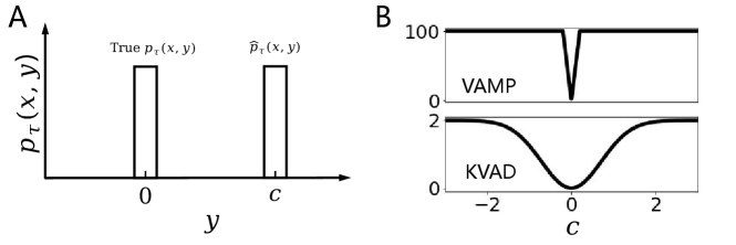
Example 2.

Let us consider a one-dimensional system with 𝕄=[5,5]\mathbb{M}=[-5,5] and ρ1(𝐱)=0.11𝐱𝕄\rho_{1}(\mathbf{x})=0.1\cdot 1_{\mathbf{x}\in\mathbb{M}}. Suppose that for a given 𝐱\mathbf{x}, pτ(𝐱,𝐲)p_{\tau}(\mathbf{x},\mathbf{y}) and p^τ(𝐱,𝐲)\hat{p}_{\tau}(\mathbf{x},\mathbf{y}) are separately uniform distributions within [0.1,0.1][-0.1,0.1] and [c0.1,c+0.1][c-0.1,c+0.1] as shown in Fig. 1A, where cc is the model parameter. In VAMP, the approximation error between the two conditional distributions are calculated as p^τ(𝐱,)pτ(𝐱,)ρ112\left\|\hat{p}_{\tau}(\mathbf{x},\cdot)-p_{\tau}(\mathbf{x},\cdot)\right\|_{\rho_{1}^{-1}}^{2}, and it can be observed from Fig. 1B that this quantity is a constant independent of cc except in a small range c[0.2,0.2]c\in[-0.2,0.2]. But kernel embedding based error p^τ(𝐱,)pτ(𝐱,)2\left\|\hat{p}_{\tau}(\mathbf{x},\cdot)-p_{\tau}(\mathbf{x},\cdot)\right\|_{\mathcal{E}}^{2} in (7) is a smooth function of cc and provides a more reasonable metric for the evaluation of cc.

Refer to caption
Figure 1: Illustration of distribution distances utilized in VAMP and KVAD. (A) The true conditional density is pτ(x,y)=51|y|0.1p_{\tau}(x,y)=5\cdot 1_{\left|y\right|\leq 0.1} for a given xx, and the approximate density is p^τ(x,y)=51|yc|0.1\hat{p}_{\tau}(x,y)=5\cdot 1_{\left|y-c\right|\leq 0.1} for the same xx. (B) The distribution distances p^τ(𝐱,)pτ(𝐱,)ρ112\left\|\hat{p}_{\tau}(\mathbf{x},\cdot)-p_{\tau}(\mathbf{x},\cdot)\right\|_{\rho_{1}^{-1}}^{2} defined in VAMP and p^τ(𝐱,)pτ(𝐱,)2\left\|\hat{p}_{\tau}(\mathbf{x},\cdot)-p_{\tau}(\mathbf{x},\cdot)\right\|_{\mathcal{E}}^{2} in KVAD with different values cc, where κ\kappa is selected as the Gaussian kernel with σ=1\sigma=1.

The following proposition shows that Eq. (7) can also be derived from the HS norm of operator error by treating 𝒫τ\mathcal{P}_{\tau} as a mapping from ρ012\mathcal{L}_{\rho_{0}^{-1}}^{2} to 2={q|q2<}\mathcal{L}_{\mathcal{E}}^{2}=\left\{q|\left\|q\right\|_{\mathcal{E}}^{2}<\infty\right\}.

Proposition 3.

If κ\kappa is a universal and bounded kernel,

  1. 1.

    𝒫τ\mathcal{P}_{\tau} is an HS operator from ρ012\mathcal{L}_{\rho_{0}^{-1}}^{2} to 2\mathcal{L}_{\mathcal{E}}^{2}, and the corresponding 𝒫^τ𝒫τHS2\left\|\mathcal{\hat{P}}_{\tau}-\mathcal{P}_{\tau}\right\|_{\mathrm{HS}}^{2} is equal to (7),

  2. 2.

    the HS norm of (𝒫^τ𝒫τ)\left(\mathcal{\hat{P}}_{\tau}-\mathcal{P}_{\tau}\right) satisfies

    𝒫^τ𝒫τHS2=[𝐟,𝐪]+𝒫τHS2,\left\|\mathcal{\hat{P}}_{\tau}-\mathcal{P}_{\tau}\right\|_{\mathrm{HS}}^{2}=-\mathcal{R}_{\mathcal{E}}\left[\mathbf{f},\mathbf{q}\right]+\left\|\mathcal{P}_{\tau}\right\|_{\mathrm{HS}}^{2},

    with

    [𝐟,𝐪]\displaystyle\mathcal{R}_{\mathcal{E}}\left[\mathbf{f},\mathbf{q}\right] =tr(2𝐂fq𝐂ff𝐂qq)\displaystyle=\mathrm{tr}\left(2\mathbf{C}_{fq}-\mathbf{C}_{ff}\mathbf{C}_{qq}\right)

    for p^τ\hat{p}_{\tau} defined by (4), where

    𝐂ff\displaystyle\mathbf{C}_{ff} =\displaystyle= 𝔼n[𝐟(𝐱n)𝐟(𝐱n)],\displaystyle\mathbb{E}_{n}\left[\mathbf{f}(\mathbf{x}_{n})\mathbf{f}(\mathbf{x}_{n})^{\top}\right],
    𝐂qq\displaystyle\mathbf{C}_{qq} =\displaystyle= [qi,qj],\displaystyle\left[\left\langle q_{i},q_{j}\right\rangle_{\mathcal{E}}\right],
    𝐂fq\displaystyle\mathbf{C}_{fq} =\displaystyle= [𝒫τ(fiρ0),qj],\displaystyle\left[\left\langle\mathcal{P}_{\tau}\left(f_{i}\rho_{0}\right),q_{j}\right\rangle_{\mathcal{E}}\right],

    are matrices of size m×mm\times m, and [𝐟,𝐪]\mathcal{R}_{\mathcal{E}}\left[\mathbf{f},\mathbf{q}\right] is called the KVAD score of 𝐟\mathbf{f} and 𝐪\mathbf{q}.

Proof.

See Appendix B. ∎

As a result of this proposition, we can find optimal 𝐟\mathbf{f} and 𝐪\mathbf{q} by maximizing \mathcal{R}_{\mathcal{E}}.

4 Approximation scheme

In this section, we derive a data-driven algorithm to estimate the optimal low-dimensional linear models based on the variational principle stated in Proposition 3.

4.1 Approximation with fixed 𝐟\mathbf{f}

We first propose a solution for the problem of finding the optimal 𝐪\mathbf{q} given that 𝐟\mathbf{f} is fixed.

Proposition 4.

If 𝐂ff=𝔼n[𝐟(𝐱n)𝐟(𝐱n)]\mathbf{C}_{ff}=\mathbb{E}_{n}\left[\mathbf{f}(\mathbf{x}_{n})\mathbf{f}(\mathbf{x}_{n})^{\top}\right] is a full-rank matrix, the solution to max𝐪[𝐟,𝐪]\max_{\mathbf{q}}\mathcal{R}_{\mathcal{E}}\left[\mathbf{f},\mathbf{q}\right] is

𝐪(𝐲)=𝐂ff1ρ0(𝐱)pτ(𝐱,𝐲)𝐟(𝐱)d𝐱\mathbf{q}(\mathbf{y})=\mathbf{C}_{ff}^{-1}\int\rho_{0}(\mathbf{x})p_{\tau}(\mathbf{x},\mathbf{y})\mathbf{f}(\mathbf{x})\mathrm{d}\mathbf{x} (8)

and

[𝐟]\displaystyle\mathcal{R}_{\mathcal{E}}\left[\mathbf{f}\right] \displaystyle\triangleq max𝐪[𝐟,𝐪]\displaystyle\max_{\mathbf{q}}\mathcal{R}_{\mathcal{E}}\left[\mathbf{f},\mathbf{q}\right] (9)
=\displaystyle= tr(𝐂ff1𝔼n,n[𝐟(𝐱n)κ(𝐲n,𝐲n)𝐟(𝐱n)]),\displaystyle\mathrm{tr}\left(\mathbf{C}_{ff}^{-1}\mathbb{E}_{n,n^{\prime}}\left[\mathbf{f}(\mathbf{x}_{n})\kappa(\mathbf{y}_{n},\mathbf{y}_{n^{\prime}})\mathbf{f}(\mathbf{x}_{n^{\prime}})^{\top}\right]\right),

where 𝔼n,n[]\mathbb{E}_{n,n^{\prime}}\left[\cdot\right] denotes the expected value with (𝐱n,𝐲n)(\mathbf{x}_{n},\mathbf{y}_{n}) and (𝐱n,𝐲n)(\mathbf{x}_{n^{\prime}},\mathbf{y}_{n^{\prime}}) independently drawn from the joint distribution of transition pairs.

Proof.

See Appendix C. ∎

As ρ0(𝐱)pτ(𝐱,𝐲)\rho_{0}(\mathbf{x})p_{\tau}(\mathbf{x},\mathbf{y}) in Eq. (8) is the joint distribution of transition pairs (𝐱n,𝐲n)(\mathbf{x}_{n},\mathbf{y}_{n}), we can get a nonparametric approximation of 𝐪\mathbf{q}

𝐪(𝐲)=1Nn𝐂ff1𝐟(𝐱n)δ𝐲n(𝐲)\mathbf{q}(\mathbf{y})=\frac{1}{N}\sum_{n}\mathbf{C}_{ff}^{-1}\mathbf{f}(\mathbf{x}_{n})\delta_{\mathbf{y}_{n}}(\mathbf{y}) (10)

by replacing the the transition pair distribution with its empirical estimate. This result gives us a linear model (1) with transition matrix

𝐊\displaystyle\mathbf{K} =\displaystyle= 1N𝐂ff1𝐟(𝐗)𝐟(𝐘)\displaystyle\frac{1}{N}\mathbf{C}_{ff}^{-1}\mathbf{f}(\mathbf{X})^{\top}\mathbf{f}(\mathbf{Y}) (11)
=\displaystyle= 𝐟(𝐗)+𝐟(𝐘)\displaystyle\mathbf{f}(\mathbf{X})^{+}\mathbf{f}(\mathbf{Y})

with 𝐟(𝐗)=(𝐟(𝐱1),,𝐟(𝐱N))N×m\mathbf{f}(\mathbf{X})=\left(\mathbf{f}(\mathbf{x}_{1}),\ldots,\mathbf{f}(\mathbf{x}_{N})\right)^{\top}\in\mathbb{R}^{N\times m} and 𝐟(𝐗)+\mathbf{f}(\mathbf{X})^{+} denoting the Penrose-Moore pseudo-inverse of 𝐟(𝐗)\mathbf{f}(\mathbf{X}), which is equal to the least square solution to the regression problem 𝐟(𝐲n)𝐊𝐟(𝐱n)\mathbf{f}(\mathbf{y}_{n})\approx\mathbf{K}^{\top}\mathbf{f}(\mathbf{x}_{n}).

4.2 Approximation with unknown 𝐟\mathbf{f}

We now consider the modeling problem with the normalization condition

p^τ(𝐱,𝐲)d𝐲=𝐟(𝐱)𝐪(𝐲)d𝐲1,\int\hat{p}_{\tau}(\mathbf{x},\mathbf{y})\mathrm{d}\mathbf{y}=\int\mathbf{f}(\mathbf{x})^{\top}\mathbf{q}(\mathbf{y})\mathrm{d}\mathbf{y}\equiv 1, (12)

where 𝐟\mathbf{f} and 𝐪\mathbf{q} are both unknown, and we make the Ansatz to represent 𝐟\mathbf{f} as linear combinations of basis functions 𝝌=(χ1,,χM)\boldsymbol{\chi}=(\chi_{1},\ldots,\chi_{M})^{\top}. Furthermore, we assume without loss of generality that the whitening transformation is applied to the basis functions so that

𝔼n[𝝌(𝐱n)]=𝟎,𝔼n[𝝌(𝐱n)𝝌(𝐱n)]=𝐈.\mathbb{E}_{n}\left[\boldsymbol{\chi}(\mathbf{x}_{n})\right]=\mathbf{0},\quad\mathbb{E}_{n}\left[\boldsymbol{\chi}(\mathbf{x}_{n})\boldsymbol{\chi}(\mathbf{x}_{n})^{\top}\right]=\mathbf{I}. (13)

(See, e.g., Appendix F in [53] for the details of whitening transformation.)

It is proved in Appendix D that there must be a solution to max𝐟[𝐟]\max_{\mathbf{f}}\mathcal{R}_{\mathcal{E}}\left[\mathbf{f}\right] under constraint (12) satisfying

f1(𝐱)1,𝐂ff=𝐈.f_{1}(\mathbf{x})\equiv 1,\quad\mathbf{C}_{ff}=\mathbf{I}. (14)

Therefore, we can model 𝐟\mathbf{f} in the form of

𝐟(𝐱)=(1,𝝌(𝐱)𝐔),𝐔m×M.\mathbf{f}(\mathbf{x})=(1,\boldsymbol{\chi}(\mathbf{x})^{\top}\mathbf{U})^{\top},\quad\mathbf{U}\in\mathbb{R}^{m\times M}. (15)

Substituting this Ansatz into the KVAD score, shows that 𝐔\mathbf{U} can be computed as the solution to the maximization problem:

max𝐔\displaystyle\max_{\mathbf{U}} (𝐔)\displaystyle\mathcal{R}_{\mathcal{E}}\left(\mathbf{U}\right)
s.t.\displaystyle\mathrm{s.t.} 𝐂ff=𝐔𝐔=𝐈\displaystyle\mathbf{C}_{ff}=\mathbf{U}^{\top}\mathbf{U}=\mathbf{I} (16)

with

(𝐔)=1N2tr(𝐔𝝌(𝐗)𝐆yy𝝌(𝐗)𝐔)+1N2𝟏𝐆yy𝟏\mathcal{R}_{\mathcal{E}}\left(\mathbf{U}\right)=\frac{1}{N^{2}}\mathrm{tr}\left(\mathbf{U}^{\top}\boldsymbol{\chi}(\mathbf{X})^{\top}\mathbf{G}_{yy}\boldsymbol{\chi}(\mathbf{X})\mathbf{U}\right)+\frac{1}{N^{2}}\mathbf{1}^{\top}\mathbf{G}_{yy}\mathbf{1} (17)

being a matrix representation of [𝐟]\mathcal{R}_{\mathcal{E}}\left[\mathbf{f}\right]. Here

𝐆yy=[κ(𝐲i,𝐲j)]N×N\mathbf{G}_{yy}=\left[\kappa\left(\mathbf{y}_{i},\mathbf{y}_{j}\right)\right]\in\mathbb{R}^{N\times N}

is the Gram matrix of 𝐘\mathbf{Y}, and 𝝌(𝐗)=(𝝌(𝐱1),,𝝌(𝐱N))N×M\boldsymbol{\chi}(\mathbf{X})=\left(\boldsymbol{\chi}(\mathbf{x}_{1}),\ldots,\boldsymbol{\chi}(\mathbf{x}_{N})\right)^{\top}\in\mathbb{R}^{N\times M}. This problem has the same form as principal component analysis problem and can be effectively can be solved via the eigendecomposition of matrix 𝝌(𝐗)𝐆yy𝝌(𝐗)\boldsymbol{\chi}(\mathbf{X})^{\top}\mathbf{G}_{yy}\boldsymbol{\chi}(\mathbf{X}) [13]. The resulting KVAD algorithm is as follows, and it can be verified that the normalization conditions (12) exactly holds for the estimated transition density (see Appendix E).

  1. 1.

    Select a set of basis function 𝝌=(χ1,,χM)\boldsymbol{\chi}=(\chi_{1},\ldots,\chi_{M})^{\top} with MmM\gg m.

  2. 2.

    Perform the whitening transformation so that (13) holds.

  3. 3.

    Perform the truncated eigendecomposition

    𝝌(𝐗)𝐆yy𝝌(𝐗)𝐔𝐒2𝐔,\boldsymbol{\chi}(\mathbf{X})^{\top}\mathbf{G}_{yy}\boldsymbol{\chi}(\mathbf{X})\approx\mathbf{U}\mathbf{S}^{2}\mathbf{U}^{\top},

    where 𝐒=diag(s1,,sm1)\mathbf{S}=\mathrm{diag}(s_{1},\ldots,s_{m-1}), s1s2sm1s_{1}\geq s_{2}\geq\ldots\geq s_{m-1} are square roots of the largest mm eigenvalues of 𝝌(𝐗)𝐆yy𝝌(𝐗)\boldsymbol{\chi}(\mathbf{X})^{\top}\mathbf{G}_{yy}\boldsymbol{\chi}(\mathbf{X}), and 𝐔=(𝐮1,,𝐮m1)\mathbf{U}=(\mathbf{u}_{1},\ldots,\mathbf{u}_{m-1}) consists of the corresponding dominant eigenvectors. This step is a bottleneck of the algorithm due to the large size Gram matrix 𝐆yy\mathbf{G}_{yy}, and the computational cost can be reduced by Nyström approximation or random fourier features [10, 36].

  4. 4.

    Calculate 𝐟\mathbf{f}, 𝐪\mathbf{q} and 𝐊\mathbf{K} by (15, 10, 11) with 𝐂ff=𝐈\mathbf{C}_{ff}=\mathbf{I}.

4.3 Component analysis

Due to the fact that f1,q1f_{1},q_{1} are non-trainable, the approximate PF operator obtained by the KVAD algorithm can be decomposed as

𝒫^τq\displaystyle\hat{\mathcal{P}}_{\tau}q =\displaystyle= f1,ρ0ρ01q1+i=2mq,fiρ0ρ01qi\displaystyle\left\langle f_{1},\rho_{0}\right\rangle_{\rho_{0}^{-1}}q_{1}+\sum_{i=2}^{m}\left\langle q,f_{i}\rho_{0}\right\rangle_{\rho_{0}^{-1}}q_{i}
=\displaystyle= q,ρ0ρ01ρ1+i=2msiq,fiρ0ρ01(si1qi).\displaystyle\left\langle q,\rho_{0}\right\rangle_{\rho_{0}^{-1}}\rho_{1}+\sum_{i=2}^{m}s_{i}\left\langle q,f_{i}\rho_{0}\right\rangle_{\rho_{0}^{-1}}\left(s_{i}^{-1}q_{i}\right).

It is worth pointing out that si,si1qi+1,fi+1ρ0s_{i},s_{i}^{-1}q_{i+1},f_{i+1}\rho_{0} obtained by KVAD algorithm are variational estimates of the iith singular value, left singular function and right singular function of the operator 𝒫~τ\tilde{\mathcal{P}}_{\tau} defined by

𝒫τq=q,ρ0ρ01ρ1+𝒫~τq,\mathcal{P}_{\tau}q=\left\langle q,\rho_{0}\right\rangle_{\rho_{0}^{-1}}\rho_{1}+\tilde{\mathcal{P}}_{\tau}q, (18)

where (𝒫~τρ0)(𝐲)0(\tilde{\mathcal{P}}_{\tau}\rho_{0})(\mathbf{y})\equiv 0. Thus, the KVAD algorithm indeed performs truncated singular value decomposition (SVD) of 𝒫~τ\tilde{\mathcal{P}}_{\tau} (see Appendix F).

At the limit case where the all singular components of 𝒫~τ\tilde{\mathcal{P}}_{\tau} are exactly estimated by KVAD, we have

Dτ(𝐱,𝐱)2\displaystyle D_{\tau}\left(\mathbf{x},\mathbf{x}^{\prime}\right)^{2} \displaystyle\triangleq pτ(𝐱,)pτ(𝐱,)2\displaystyle\left\|p_{\tau}(\mathbf{x},\cdot)-p_{\tau}(\mathbf{x}^{\prime},\cdot)\right\|_{\mathcal{E}}^{2} (19)
=\displaystyle= i=1m1si2(fi+1(𝐱)fi+1(𝐱))2\displaystyle\sum_{i=1}^{m-1}s_{i}^{2}\left(f_{i+1}(\mathbf{x})-f_{i+1}(\mathbf{x}^{\prime})\right)^{2}

for all 𝐱,𝐱𝕄\mathbf{x},\mathbf{x}^{\prime}\in\mathbb{M}. The distance DτD_{\tau} measures the dynamical similarity of two points in the state space, and can be approximated by the Euclidean distance derived from coordinates (s1f2(𝐱),,sm1fm(𝐱))(s_{1}f_{2}(\mathbf{x}),\ldots,s_{m-1}f_{m}(\mathbf{x}))^{\top} as shown in (19). Hence, KVAD provides an ideal low-dimensional embedding of system dynamics, and can be reinterpreted a variant of the diffusion mapping method for dynamical model reduction [5] (see Appendix G).

5 Relationship with Other Methods

5.1 EDMD and VAMP

It can be seen from (11) that the optimal linear model obtained by KVAD is consistent with the model of EDMD [49] for given feature functions 𝐟\mathbf{f}. However, the optimization and the dimension reduction of the observables are not considered in the conventional EDMD.

Both VAMP [53] and KVAD solve this problem by variational formulations of modeling errors. As analyzed in Sections 2.1 and 3, KVAD is applicable to more general systems, including deterministic systems, compared to VAMP. Moreover, VAMP needs to represent both 𝐟\mathbf{f} and 𝐪\mathbf{q} by parametric models for dynamical approximation, whereas KVAD can obtain the optimal 𝐪\mathbf{q} from data without any parametric model for given 𝐟\mathbf{f}. Our numerical experiments (see Section 6) show that KVAD can often provide more accurate low-dimensional models than VAMP when the same Ansatz basis functions are used.

5.2 Conditional mean embedding, kernel EDMD and kernel CCA

For given two random variables 𝐱\mathbf{x} and 𝐲\mathbf{y}, the conditional mean embedding proposed in [46] characterizes the conditional distribution of 𝐲\mathbf{y} for given 𝐱\mathbf{x} by the conditional embedding operator 𝒞𝐲|𝐱\mathcal{C}_{\mathbf{y}|\mathbf{x}} with

𝔼[φ(𝐲)|𝐱]=𝒞𝐲|𝐱φ(𝐱),\mathbb{E}[\varphi(\mathbf{y})|\mathbf{x}]=\mathcal{C}_{\mathbf{y}|\mathbf{x}}\varphi(\mathbf{x}),

where φ\varphi denotes the kernel mapping and 𝒞𝐲|𝐱\mathcal{C}_{\mathbf{y}|\mathbf{x}} can be consistently estimated from data. When applied to dynamical data, this method has the same form as the kernel EDMD and its variants [42, 16, 15], and is indeed a specific case of KVAD with Ansatz functions 𝝌=φ\boldsymbol{\chi}=\varphi and dimension m=Nm=N (see Appendix H).

In addition, for most kernel based dynamical modeling methods, the dimension reduction problem is not thoroughly investigated. In [18], a kernel method for eigendecomposition of transfer operators (including PF operators and Koopman operators) was developed. But as analyzed in [53], the dominant eigen-components may not yield an accurate low-dimensional dynamical model. Kernel canonical correlation analysis (CCA) [22] can overcome this problem as a kernelization of VAMP, but it is also applicable only if 𝒫τ\mathcal{P}_{\tau} is a compact operator from ρ012\mathcal{L}_{\rho_{0}^{-1}}^{2} to ρ112\mathcal{L}_{\rho_{1}^{-1}}^{2}.

Compared to the previous kernel methods, KVAD has more flexibility in model choice, where the dimension and model class of 𝐟\mathbf{f} can be arbitrarily selected according to practical requirements.

6 Numerical experiments

In what follows, we demonstrate the benefits of the KVAD method for studies of nonlinear dynamical systems by two examples, and compare the results from KVAD with VAMP and kernel EDMD, where the basis functions in VAMP and kernel functions in kernel EDMD are the same as those in KVAD. For kernel EDMD, the low-dimensional linear model is achieved by leading eigenvalues and eigenfunctions as in [18], which characterizes invariant subspaces of systems.

Example 5.

Van der Pol oscillator, which is a two-dimensional system governed by

dxt\displaystyle\mathrm{d}x_{t} =\displaystyle= ytdt+ξdwx,t,\displaystyle y_{t}\mathrm{d}t+\xi\cdot\mathrm{d}w_{x,t},
dyt\displaystyle\mathrm{d}y_{t} =\displaystyle= (2(0.2xt2)ytxt)dt+ξdwy,t,\displaystyle\left(2\left(0.2-x_{t}^{2}\right)y_{t}-x_{t}\right)\mathrm{d}t+\xi\cdot\mathrm{d}w_{y,t},

where wx,tw_{x,t} and wy,tw_{y,t} are standard Wiener processes. The flow field of this system for ξ=0\xi=0 is depicted in Fig. 2A. We generate N=2000N=2000 transition pairs for modeling, where the lag time τ=0.2\tau=0.2, 𝐗=(𝐱1,,𝐱N)\mathbf{X}=(\mathbf{x}_{1},\ldots,\mathbf{x}_{N})^{\top} are randomly drawn from [1.5,1.5]2[-1.5,1.5]^{2}, and 𝐘=(𝐲1,,𝐲N)\mathbf{Y}=(\mathbf{y}_{1},\ldots,\mathbf{y}_{N})^{\top} are obtained by the Euler-Maruyama scheme with step size 0.010.01.

Example 6.

Lorenz system defined by

dxt\displaystyle\mathrm{d}x_{t} =\displaystyle= 10(ytxt)dt+ξxtdwx,t,\displaystyle 10(y_{t}-x_{t})\mathrm{d}t+\xi\cdot x_{t}\cdot\mathrm{d}w_{x,t},
dyt\displaystyle\mathrm{d}y_{t} =\displaystyle= (28xtytxtzt)dt+ξytdwy,t,\displaystyle\left(28x_{t}-y_{t}-x_{t}z_{t}\right)\mathrm{d}t+\xi\cdot y_{t}\cdot\mathrm{d}w_{y,t},
dzt\displaystyle\mathrm{d}z_{t} =\displaystyle= (xtyt83zt)dt+ξztdwz,t,\displaystyle\left(x_{t}y_{t}-\frac{8}{3}z_{t}\right)\mathrm{d}t+\xi\cdot z_{t}\cdot\mathrm{d}w_{z,t},

with wx,t,wy,t,wz,tw_{x,t},w_{y,t},w_{z,t} being standard Wiener processes. Fig. 2B plots a trajectory of this system in the state space with ξ=0\xi=0. We sample 20002000 transition pairs from a simulation trajectory with length 200200 and lag time τ=0.1\tau=0.1 as training data for each ξ\xi, and perform simulations by the Euler-Maruyama scheme with step size 0.0050.005.

In both examples, the feature mapping 𝐟\mathbf{f} is represented by basis functions

χi(𝐱)=exp((𝜽i𝐱+bi)2),fori=1,,500\chi_{i}(\mathbf{x})=\exp\left(-\left(\boldsymbol{\theta}_{i}^{\top}\mathbf{x}+b_{i}\right)^{2}\right),fori=1,\ldots,500

with all components of 𝜽i\boldsymbol{\theta}_{i} and bib_{i} randomly drawn from [1,1][-1,1], which are widely used in shallow neural networks [12, 7]. The kernel κ\kappa is selected as the Gaussian kernel with σ=1.5\sigma=1.5 for the oscillator and 1010 for the Lorenz system.

Fig. 2 shows estimates of singular values of 𝒫~τ:ρ0122\tilde{\mathcal{P}}_{\tau}:\mathcal{L}_{\rho_{0}^{-1}}^{2}\to\mathcal{L}_{\mathcal{E}}^{2} (KVAD), singular values of 𝒫τ:ρ012ρ112\mathcal{P}_{\tau}:\mathcal{L}_{\rho_{0}^{-1}}^{2}\to\mathcal{L}_{\rho_{1}^{-1}}^{2} (VAMP) and absolute values of eigenvalues of 𝒫τ\mathcal{P}_{\tau} (kernel EDMD) with different noise parameters, where singular values must be nonnegative real numbers but eigenvalues could be complex or negative. We see that the singular values and eigenvalues given by VAMP and kernel EDMD decay very slowly. Hence, it is difficult to extract an accurate model from the estimation results of VAMP and kernel EDMD for a small mm. Especially for VAMP, a large number of singular values are close to 11 as analyzed in Proposition 1 when the systems are deterministic with ξ=0\xi=0. In contrast, the singular values utilized in KVAD rapidly converges to zero, which implies one can effectively extract the essential part of dynamics from a small number of feature mappings.

The first two singular components of 𝒫~τ\tilde{\mathcal{P}}_{\tau} for ξ=0\xi=0 obtained by KVAD are shown in Fig. 3 (see Section 4.3).555The qiq_{i} is approximated by multiple delta functions and hard to visualize. It can be observed that f1,f2f_{1},f_{2} of the oscillator characterize transitions between left-right and up-down areas separately. Those of the Lorenz systems are related to the two attractor lobes and the transition areas.

It is interesting to note that the singular values of 𝒫~τ\tilde{\mathcal{P}}_{\tau} given by KVAD are slightly influenced by ξ\xi as illustrated in Fig. 2. Our numerical experience also show that the right singular functions remain almost unchanged for different ξ\xi (see Fig. 5 in Appendix I). This phenomenon can be partially explained by the fact that the variational score ϵ\mathcal{R}_{\epsilon} estimated by (17) is not sensitive to small perturbations of 𝐘\mathbf{Y} if the bandwidth of the kernel is large. More thorough investigations on this phenomenon will be performed in future.

Refer to caption
Figure 2: (A.1) Flow map of the Van der Pol oscillator, where the arrows represent directions of (dxt,dyt)(\mathrm{d}x_{t},\mathrm{d}y_{t}) with ξ=0\xi=0. (B.1) A typical trajectory of the Lorenz system with ξ=0\xi=0 generated by the Euler-Maruyama scheme. (A.2 and B.2) Estimated singular values and absolute values of eigenvalues of the oscillator and the Lorenz system. Red lines represent singular values of 𝒫~τ\tilde{\mathcal{P}}_{\tau} estimated by KVAD (see (18)), green lines singular values of 𝒫τ\mathcal{P}_{\tau} estimated by VAMP, red lines absolute values of eigenvalues of 𝒫τ\mathcal{P}_{\tau} estimated by kernel EDMD, solid lines estimates with ξ=0\xi=0, and dashed lines those with ξ=0.2\xi=0.2 (oscillator) and 0.50.5 (Lorenz system). Notice the total number of spectral components changes in different cases due to the rank truncation in implementations of SVD and pseudo inverse.
Refer to caption
Figure 3: The first two singular components computed by KVAD, where ξ=0\xi=0, sis_{i} is the estimate of the iith singular value of 𝒫~τ\tilde{\mathcal{P}}_{\tau} and fiρ0f_{i}\cdot\rho_{0} the estimate of the corresponding right singular function (see Section 4.3). (A) The oscillator. (B) The Lorenz system.

In order to quantitively evaluate the performance of the three methods, we define the following trajectory reconstruction error:

error=1Ll=1L𝐱lτ𝔼model[𝐱lτ|𝐱0],\mathrm{error}=\sqrt{\frac{1}{L}\sum_{l=1}^{L}\left\|\mathbf{x}_{l\tau}-\mathbb{E}_{\mathrm{model}}[\mathbf{x}_{l\tau}|\mathbf{x}_{0}]\right\|},

where 𝐱t\mathbf{x}_{t} is the true trajectory data and 𝔼model[𝐱t|𝐱0]\mathbb{E}_{\mathrm{model}}[\mathbf{x}_{t}|\mathbf{x}_{0}] is the conditional mean value of 𝐱t\mathbf{x}_{t} obtained by the model. The average error over multiple replicate simulations is minimized if and only if 𝔼model[𝐱lτ|𝐱0]\mathbb{E}_{\mathrm{model}}[\mathbf{x}_{l\tau}|\mathbf{x}_{0}] equals to the exact conditional mean value of 𝐱lτ\mathbf{x}_{l\tau} for all ll. For all the three methods,

𝔼model[𝐱lτ|𝐱0]\displaystyle\mathbb{E}_{\mathrm{model}}[\mathbf{x}_{l\tau}|\mathbf{x}_{0}] =𝐆𝔼model[𝐟(𝐱(l1)τ)|𝐱0]\displaystyle=\mathbf{G}^{\top}\mathbb{E}_{\mathrm{model}}\left[\mathbf{f}(\mathbf{x}_{(l-1)\tau})|\mathbf{x}_{0}\right]
=\displaystyle= (𝐊l1𝐆)𝐟(𝐱0),\displaystyle\left(\mathbf{K}^{l-1}\mathbf{G}\right)^{\top}\mathbf{f}(\mathbf{x}_{0}),

where 𝐆\mathbf{G} is the least square solution to the regression problem 𝐱t+τ𝐆𝐟(𝐱t)\mathbf{x}_{t+\tau}\approx\mathbf{G}^{\top}\mathbf{f}(\mathbf{x}_{t}) [49]. Fig. 4 summarizes of reconstruction errors of the two systems obtained with different choices of the model dimension mm and noise parameter ξ\xi, and the superiority of our KVAD is clearly shown.

Refer to caption
Figure 4: (A) Reconstruction errors of the oscillator, where L=50L=50 and 𝐱0\mathbf{x}_{0} is randomly drawn in [1.5,1.5]2[-1.5,1.5]^{2}. (B) Reconstruction errors of the Lorenz. Here L=8L=8, 𝐱0\mathbf{x}_{0} is randomly sampled from a long simulation trajectory, and the trajectory is independent of the training data. Error bars represent standard deviations calculated from 100 bootstrapping replicates of simulations.

7 Conclusion

In this paper, we combine the kernel embedding technique with the variational principle for transfer operators. This provides a powerful and flexible tool for low-dimensional approximation of dynamical system, and effectively addresses the shortcomings and limitations of the existing variational approach. In the proposed KVAD framework, a bounded and well defined distance measure of transfer operators is developed based on kernel embedding of transition densities, and the corresponding variational optimization approach can be applied to a broader range of dynamical systems than the existing variational approaches.

Our future work includes the convergence analysis of KVAD and optimization of kernel functions. From the algorithmic point of view, the main remaining question is how to efficiently perform KVAD learning from big data with deep neural networks. It will be also interesting to apply KVAD to multi-ensemble Markov models [55] for data analysis of enhanced sampling.

Appendix

For convenience of notation, we define

𝐚,𝐛=[ai,bj]n1×n2\left\langle\mathbf{a},\mathbf{b}^{\top}\right\rangle=\left[\left\langle a_{i},b_{j}\right\rangle\right]\in\mathbb{R}^{n_{1}\times n_{2}}

and

𝒫τ𝐚=(𝒫τa1,,𝒫τan1)\mathcal{P}_{\tau}\mathbf{a}=(\mathcal{P}_{\tau}a_{1},\ldots,\mathcal{P}_{\tau}a_{n_{1}})^{\top}

for 𝐚=(a1,,an1)\mathbf{a}=(a_{1},\ldots,a_{n_{1}})^{\top}, 𝐛=(b1,,bn1)\mathbf{b}=(b_{1},\ldots,b_{n_{1}})^{\top} and an inner product ,\left\langle\cdot,\cdot\right\rangle.

Appendix A Proof of Proposition 1

The proof of first conclusion is given in Appendices A.5 and B of [53], and we prove here the second conclusion.

We first show [𝐟,𝐪]m\mathcal{R}\left[\mathbf{f},\mathbf{q}\right]\leq m. Because 𝔼n[𝐟(𝐱n)𝐟(𝐱n)]\mathbb{E}_{n}\left[\mathbf{f}(\mathbf{x}_{n})\mathbf{f}(\mathbf{x}_{n})^{\top}\right] is a positive semi-definite matrices, it can be decomposed as

𝔼n[𝐟(𝐱n)𝐟(𝐱n)]\displaystyle\mathbb{E}_{n}\left[\mathbf{f}(\mathbf{x}_{n})\mathbf{f}(\mathbf{x}_{n})^{\top}\right] =\displaystyle= 𝐐𝐃𝐐,\displaystyle\mathbf{Q}\mathbf{D}\mathbf{Q}^{\top}, (20)

where 𝐐\mathbf{Q} is a orthogonal matrix and 𝐃\mathbf{D} is a diagonal matrix. Let 𝐟=(f1,,fm)=𝐐𝐟\mathbf{f}^{\prime}=(f_{1}^{\prime},\ldots,f_{m}^{\prime})^{\top}=\mathbf{Q}^{\top}\mathbf{f} and 𝐠=(g1,,gm)=𝐐𝐠\mathbf{g}^{\prime}=(g_{1}^{\prime},\ldots,g_{m}^{\prime})^{\top}=\mathbf{Q}^{\top}\mathbf{g}, we have

[𝐟,𝐪]\displaystyle\mathcal{R}\left[\mathbf{f},\mathbf{q}\right] =\displaystyle= tr(2𝔼n[𝐐𝐟(𝐱n)𝐠(𝐲n)𝐐]𝔼n[𝐐𝐟(𝐱n)𝐟(𝐱n)𝐐]𝔼n[𝐐𝐠(𝐲n)𝐠(𝐲n)𝐐])\displaystyle\mathrm{tr}\left(2\mathbb{E}_{n}\left[\mathbf{Q}^{\top}\mathbf{f}(\mathbf{x}_{n})\mathbf{g}(\mathbf{y}_{n})^{\top}\mathbf{Q}\right]-\mathbb{E}_{n}\left[\mathbf{Q}^{\top}\mathbf{f}(\mathbf{x}_{n})\mathbf{f}(\mathbf{x}_{n})^{\top}\mathbf{Q}\right]\mathbb{E}_{n}\left[\mathbf{Q}^{\top}\mathbf{g}(\mathbf{y}_{n})\mathbf{g}(\mathbf{y}_{n})^{\top}\mathbf{Q}\right]\right)
=\displaystyle= tr(2𝔼n[𝐟(𝐱n)𝐠(𝐲n)]𝔼n[𝐟(𝐱n)𝐟(𝐱n)]𝔼n[𝐠(𝐲n)𝐠(𝐲n)])\displaystyle\mathrm{tr}\left(2\mathbb{E}_{n}\left[\mathbf{f}^{\prime}(\mathbf{x}_{n})\mathbf{g}^{\prime}(\mathbf{y}_{n})^{\top}\right]-\mathbb{E}_{n}\left[\mathbf{f}^{\prime}(\mathbf{x}_{n})\mathbf{f}^{\prime}(\mathbf{x}_{n})^{\top}\right]\mathbb{E}_{n}\left[\mathbf{g}^{\prime}(\mathbf{y}_{n})\mathbf{g}^{\prime}(\mathbf{y}_{n})^{\top}\right]\right)
=\displaystyle= i=1m2𝔼n[fi(𝐱n)gi(𝐲n)]𝔼n[fi(𝐱n)2]𝔼n[gi(𝐱n)2]\displaystyle\sum_{i=1}^{m}2\mathbb{E}_{n}\left[f_{i}^{\prime}(\mathbf{x}_{n})g_{i}^{\prime}(\mathbf{y}_{n})\right]-\mathbb{E}_{n}\left[f_{i}^{\prime}(\mathbf{x}_{n})^{2}\right]\mathbb{E}_{n}\left[g_{i}^{\prime}(\mathbf{x}_{n})^{2}\right]
\displaystyle\leq i=1m2𝔼n[fi(𝐱n)gi(𝐲n)]𝔼n[fi(𝐱n)gi(𝐲n)]2\displaystyle\sum_{i=1}^{m}2\mathbb{E}_{n}\left[f_{i}^{\prime}(\mathbf{x}_{n})g_{i}^{\prime}(\mathbf{y}_{n})\right]-\mathbb{E}_{n}\left[f_{i}^{\prime}(\mathbf{x}_{n})g_{i}^{\prime}(\mathbf{y}_{n})\right]^{2}
\displaystyle\leq m.\displaystyle m.

Under the assumption of 𝔼n[𝐠(𝐲n)𝐠(𝐲n)]=𝐈\mathbb{E}_{n}\left[\mathbf{g}(\mathbf{y}_{n})\mathbf{g}(\mathbf{y}_{n})^{\top}\right]=\mathbf{I} and fi(𝐱)=gi(Θτ(𝐱))f_{i}(\mathbf{x})=g_{i}(\Theta_{\tau}(\mathbf{x})), we have

giρ1,gjρ1ρ11\displaystyle\left\langle g_{i}\rho_{1},g_{j}\rho_{1}\right\rangle_{\rho_{1}^{-1}} =\displaystyle= ρ1(𝐲)gi(𝐲)gj(𝐲)d𝐲\displaystyle\int\rho_{1}(\mathbf{y})g_{i}(\mathbf{y})g_{j}(\mathbf{y})\mathrm{d}\mathbf{y}
=\displaystyle= 𝔼n[gi(𝐲n)gj(𝐲n)]\displaystyle\mathbb{E}_{n}\left[g_{i}(\mathbf{y}_{n})g_{j}(\mathbf{y}_{n})\right]
=\displaystyle= 1i=j\displaystyle 1_{i=j}

and

𝔼n[𝐟(𝐱n)𝐟(𝐱n)]\displaystyle\mathbb{E}_{n}\left[\mathbf{f}(\mathbf{x}_{n})\mathbf{f}(\mathbf{x}_{n})^{\top}\right] =\displaystyle= 𝔼n[𝐠(Θ(𝐱n))𝐠(Θ(𝐱n))]\displaystyle\mathbb{E}_{n}\left[\mathbf{g}(\Theta(\mathbf{x}_{n}))\mathbf{g}(\Theta(\mathbf{x}_{n}))^{\top}\right]
=\displaystyle= 𝔼n[𝐠(𝐲n)𝐠(𝐲n)]=𝐈\displaystyle\mathbb{E}_{n}\left[\mathbf{g}(\mathbf{y}_{n})\mathbf{g}(\mathbf{y}_{n})^{\top}\right]=\mathbf{I}

with 𝐠=(g1,,gm)\mathbf{g}=(g_{1},\ldots,g_{m})^{\top} by considering that 𝐲n=Θτ(𝐱n)\mathbf{y}_{n}=\Theta_{\tau}(\mathbf{x}_{n}). Consequently,

[𝐟,𝐪]\displaystyle\mathcal{R}\left[\mathbf{f},\mathbf{q}\right] =\displaystyle= tr(2𝔼n[𝐟(𝐱n)𝐠(𝐲n)]𝐈)\displaystyle\mathrm{tr}\left(2\mathbb{E}_{n}\left[\mathbf{f}(\mathbf{x}_{n})\mathbf{g}(\mathbf{y}_{n})^{\top}\right]-\mathbf{I}\right)
=\displaystyle= tr(2𝔼n[𝐠(𝐲n)𝐠(𝐲n)]𝐈)\displaystyle\mathrm{tr}\left(2\mathbb{E}_{n}\left[\mathbf{g}(\mathbf{y}_{n})\mathbf{g}(\mathbf{y}_{n})^{\top}\right]-\mathbf{I}\right)
=\displaystyle= m,\displaystyle m,

which yields the second conclusion of this proposition.

Appendix B Proof of Proposition 3

Let {e1,e2,}\{e_{1},e_{2},\ldots\} be an orthonormal basis of ρ012\mathcal{L}_{\rho_{0}^{-1}}^{2}. We have

k𝒫^τek,𝒫τekκ\displaystyle\sum_{k}\left\langle\hat{\mathcal{P}}_{\tau}e_{k},\mathcal{P}_{\tau}e_{k}\right\rangle_{\kappa} =\displaystyle= kpτ(𝐱,𝐲)ek(𝐱)𝝋(𝐲),𝝋(𝐲)p^τ(𝐱,𝐲)ek(𝐱)d𝐱d𝐱d𝐲d𝐲\displaystyle\sum_{k}\iiiint p_{\tau}(\mathbf{x},\mathbf{y})e_{k}(\mathbf{x})\left\langle\boldsymbol{\varphi}(\mathbf{y}),\boldsymbol{\varphi}(\mathbf{y}^{\prime})\right\rangle_{\mathbb{H}}\hat{p}_{\tau}(\mathbf{x}^{\prime},\mathbf{y}^{\prime})e_{k}(\mathbf{x}^{\prime})\mathrm{d}\mathbf{x}\mathrm{d}\mathbf{x}^{\prime}\mathrm{d}\mathbf{y}\mathrm{d}\mathbf{y}^{\prime}
=\displaystyle= κ(𝐲,𝐲)kpτ(𝐱,𝐲)ek(𝐱)p^τ(𝐱,𝐲)ek(𝐱)d𝐱d𝐱d𝐲d𝐲\displaystyle\iiiint\kappa(\mathbf{y},\mathbf{y}^{\prime})\cdot\sum_{k}p_{\tau}(\mathbf{x},\mathbf{y})e_{k}(\mathbf{x})\hat{p}_{\tau}(\mathbf{x}^{\prime},\mathbf{y}^{\prime})e_{k}(\mathbf{x}^{\prime})\mathrm{d}\mathbf{x}\mathrm{d}\mathbf{x}^{\prime}\mathrm{d}\mathbf{y}\mathrm{d}\mathbf{y}^{\prime}
=\displaystyle= κ(𝐲,𝐲)(kpτ(𝐱,𝐲)ek(𝐱)p^τ(𝐱,𝐲)ek(𝐱)d𝐱d𝐱)d𝐲d𝐲\displaystyle\iint\kappa(\mathbf{y},\mathbf{y}^{\prime})\cdot\left(\sum_{k}\iint p_{\tau}(\mathbf{x},\mathbf{y})e_{k}(\mathbf{x})\hat{p}_{\tau}(\mathbf{x}^{\prime},\mathbf{y}^{\prime})e_{k}(\mathbf{x}^{\prime})\mathrm{d}\mathbf{x}\mathrm{d}\mathbf{x}^{\prime}\right)\mathrm{d}\mathbf{y}\mathrm{d}\mathbf{y}^{\prime}
=\displaystyle= κ(𝐲,𝐲)k(pτ(𝐱,𝐲)ek(𝐱)d𝐱)\displaystyle\iint\kappa(\mathbf{y},\mathbf{y}^{\prime})\cdot\sum_{k}\left(\int p_{\tau}(\mathbf{x},\mathbf{y})e_{k}(\mathbf{x})\mathrm{d}\mathbf{x}\right)
\displaystyle\cdot (p^τ(𝐱,𝐲)ek(𝐱)d𝐱)d𝐲d𝐲\displaystyle\left(\int\hat{p}_{\tau}(\mathbf{x}^{\prime},\mathbf{y}^{\prime})e_{k}(\mathbf{x}^{\prime})\mathrm{d}\mathbf{x}^{\prime}\right)\mathrm{d}\mathbf{y}\mathrm{d}\mathbf{y}^{\prime}
=\displaystyle= κ(𝐲,𝐲)pτ(,𝐲)ρ0(),p^τ(,𝐲)ρ0()ρ01d𝐲d𝐲\displaystyle\iint\kappa(\mathbf{y},\mathbf{y}^{\prime})\cdot\left\langle p_{\tau}(\cdot,\mathbf{y})\rho_{0}(\cdot),\hat{p}_{\tau}(\cdot,\mathbf{y})\rho_{0}(\cdot)\right\rangle_{\rho_{0}^{-1}}\mathrm{d}\mathbf{y}\mathrm{d}\mathbf{y}^{\prime}
=\displaystyle= ρ0(𝐱)pτ(𝐱,𝐲)p^τ(𝐱,𝐲)κ(𝐲,𝐲)d𝐱d𝐲d𝐲\displaystyle\iint\int\rho_{0}(\mathbf{x})\cdot p_{\tau}(\mathbf{x},\mathbf{y})\hat{p}_{\tau}(\mathbf{x},\mathbf{y}^{\prime})\cdot\kappa(\mathbf{y},\mathbf{y}^{\prime})\mathrm{d}\mathbf{x}\mathrm{d}\mathbf{y}\mathrm{d}\mathbf{y}^{\prime}
=\displaystyle= ρ0(𝐱)pτ(𝐱,),p^τ(𝐱,)d𝐱.\displaystyle\int\rho_{0}(\mathbf{x})\left\langle p_{\tau}(\mathbf{x},\cdot),\hat{p}_{\tau}(\mathbf{x},\cdot)\right\rangle_{\mathcal{E}}\mathrm{d}\mathbf{x}.

Therefore, 𝒫τ\mathcal{P}_{\tau} is an HS operator with

𝒫τHS2\displaystyle\left\|\mathcal{P}_{\tau}\right\|_{\mathrm{HS}}^{2} =\displaystyle= k𝒫τek,𝒫τek\displaystyle\sum_{k}\left\langle\mathcal{P}_{\tau}e_{k},\mathcal{P}_{\tau}e_{k}\right\rangle_{\mathcal{E}}
=\displaystyle= ρ0(𝐱)pτ(𝐱,)2d𝐱B\displaystyle\int\rho_{0}(\mathbf{x})\left\|p_{\tau}(\mathbf{x},\cdot)\right\|_{\mathcal{E}}^{2}\mathrm{d}\mathbf{x}\leq B

if κ\kappa is bounded by BB, and

𝒫τ𝒫^τHS2\displaystyle\left\|\mathcal{P}_{\tau}-\hat{\mathcal{P}}_{\tau}\right\|_{\mathrm{HS}}^{2} =\displaystyle= k(𝒫τ𝒫^τ)ek,(𝒫τ𝒫^τ)ekκ\displaystyle\sum_{k}\left\langle\left(\mathcal{P}_{\tau}-\hat{\mathcal{P}}_{\tau}\right)e_{k},\left(\mathcal{P}_{\tau}-\hat{\mathcal{P}}_{\tau}\right)e_{k}\right\rangle_{\kappa}
=\displaystyle= 𝒟(𝒫^τ,𝒫τ)2.\displaystyle\mathcal{D}\left(\mathcal{\hat{P}}_{\tau},\mathcal{P}_{\tau}\right)^{2}.

If p^τ(𝐱,𝐲)=𝐟(𝐱)𝐪(𝐲)\hat{p}_{\tau}(\mathbf{x},\mathbf{y})=\mathbf{f}(\mathbf{x})^{\top}\mathbf{q}(\mathbf{y}), we get

𝒫^τHS2\displaystyle\left\|\hat{\mathcal{P}}_{\tau}\right\|_{\mathrm{HS}}^{2} =\displaystyle= ρ0(𝐱)𝐟(𝐱)𝐪(𝐲)κ(𝐲,𝐲)𝐪(𝐲)𝐟(𝐱)d𝐱d𝐲d𝐲\displaystyle\iiint\rho_{0}(\mathbf{x})\mathbf{f}(\mathbf{x})^{\top}\mathbf{q}(\mathbf{y})\kappa\left(\mathbf{y},\mathbf{y}^{\prime}\right)\mathbf{q}(\mathbf{y}^{\prime})^{\top}\mathbf{f}(\mathbf{x})\mathrm{d}\mathbf{x}\mathrm{d}\mathbf{y}\mathrm{d}\mathbf{y}^{\prime}
=\displaystyle= tr(𝐂ff𝐂qq),\displaystyle\mathrm{tr}\left(\mathbf{C}_{ff}\mathbf{C}_{qq}\right),
k𝒫^τek,𝒫τekκ\displaystyle\sum_{k}\left\langle\hat{\mathcal{P}}_{\tau}e_{k},\mathcal{P}_{\tau}e_{k}\right\rangle_{\kappa} =\displaystyle= ρ0(𝐱)pτ(𝐱,𝐲)𝐪(𝐲)𝐟(𝐱)κ(𝐲,𝐲)d𝐱d𝐲d𝐲\displaystyle\int\int\int\rho_{0}(\mathbf{x})\cdot p_{\tau}(\mathbf{x},\mathbf{y})\mathbf{q}(\mathbf{y}^{\prime})^{\top}\mathbf{f}(\mathbf{x})\cdot\kappa(\mathbf{y},\mathbf{y}^{\prime})\mathrm{d}\mathbf{x}\mathrm{d}\mathbf{y}\mathrm{d}\mathbf{y}^{\prime}
=\displaystyle= tr(𝐂fq),\displaystyle\mathrm{tr}\left(\mathbf{C}_{fq}\right),

and

𝒫τ𝒫^τHS2=[𝐟,𝐪]+𝒫τHS2.\left\|\mathcal{P}_{\tau}-\hat{\mathcal{P}}_{\tau}\right\|_{\mathrm{HS}}^{2}=-\mathcal{R}_{\mathcal{E}}\left[\mathbf{f},\mathbf{q}\right]+\left\|\mathcal{P}_{\tau}\right\|_{\mathrm{HS}}^{2}.

Appendix C Proof of Proposition 4

Let us first consider the case where 𝐂ff=𝐈\mathbf{C}_{ff}=\mathbf{I}. Then

[𝐟,𝐪]\displaystyle\mathcal{R_{E}}[\mathbf{f},\mathbf{q}] =\displaystyle= tr(𝐪,𝐪2𝐪,𝒫τ(𝐟ρ0))\displaystyle-\mathrm{tr}\left(\left\langle\mathbf{q},\mathbf{q}^{\top}\right\rangle_{\mathcal{E}}-2\left\langle\mathbf{q},\mathcal{P}_{\tau}\left(\mathbf{f}\rho_{0}\right)^{\top}\right\rangle_{\mathcal{E}}\right)
=\displaystyle= tr(𝐪𝒫τ(𝐟ρ0),(𝐪𝒫τ(𝐟ρ0))𝒫τ(𝐟ρ0),𝒫τ(𝐟ρ0))\displaystyle-\mathrm{tr}\left(\left\langle\mathbf{q}-\mathcal{P}_{\tau}\left(\mathbf{f}\rho_{0}\right),\left(\mathbf{q}-\mathcal{P}_{\tau}\left(\mathbf{f}\rho_{0}\right)\right)^{\top}\right\rangle_{\mathcal{E}}-\left\langle\mathcal{P}_{\tau}\left(\mathbf{f}\rho_{0}\right),\mathcal{P}_{\tau}\left(\mathbf{f}\rho_{0}\right)^{\top}\right\rangle_{\mathcal{E}}\right)
=\displaystyle= iqi𝒫τ(fiρ0)2+i𝒫τ(fiρ0)2,\displaystyle-\sum_{i}\left\|q_{i}-\mathcal{P}_{\tau}\left(f_{i}\rho_{0}\right)\right\|_{\mathcal{E}}^{2}+\sum_{i}\left\|\mathcal{P}_{\tau}\left(f_{i}\rho_{0}\right)\right\|_{\mathcal{E}}^{2},

which leads to

argmax𝐪[𝐟,𝐪]\displaystyle\arg\max_{\mathbf{q}}\mathcal{R_{E}}[\mathbf{f},\mathbf{q}] =\displaystyle= 𝒫τ(𝐟ρ0)\displaystyle\mathcal{P}_{\tau}\left(\mathbf{f}\rho_{0}\right)
=\displaystyle= ρ0(𝐱)pτ(𝐱,)𝐟(𝐱)d𝐱\displaystyle\int\rho_{0}(\mathbf{x})p_{\tau}(\mathbf{x},\cdot)\mathbf{f}(\mathbf{x})\mathrm{d}\mathbf{x}

and

[𝐟]\displaystyle\mathcal{R_{E}}[\mathbf{f}] =\displaystyle= 𝒫τ(𝐟ρ0)2\displaystyle\left\|\mathcal{P}_{\tau}\left(\mathbf{f}\rho_{0}\right)\right\|_{\mathcal{E}}^{2}
=\displaystyle= tr(𝔼n,n[𝐟(𝐱n)κ(𝐲n,𝐲n)𝐟(𝐱n)]).\displaystyle\mathrm{tr}\left(\mathbb{E}_{n,n^{\prime}}\left[\mathbf{f}(\mathbf{x}_{n})\kappa(\mathbf{y}_{n},\mathbf{y}_{n^{\prime}})\mathbf{f}(\mathbf{x}_{n^{\prime}})^{\top}\right]\right).

We now suppose that 𝐂ff𝐈\mathbf{C}_{ff}\neq\mathbf{I} and let

𝐟\displaystyle\mathbf{f}^{\prime} =\displaystyle= 𝐂ff12𝐟,\displaystyle\mathbf{C}_{ff}^{-\frac{1}{2}}\mathbf{f},
𝐪\displaystyle\mathbf{q}^{\prime} =\displaystyle= 𝐂ff12𝐪.\displaystyle\mathbf{C}_{ff}^{\frac{1}{2}}\mathbf{q}.

Becuase 𝐟,𝐟ρ0=𝐈\left\langle\mathbf{f}^{\prime},\mathbf{f}^{\prime\top}\right\rangle_{\rho_{0}}=\mathbf{I}, we have

argmax𝐪[𝐟,𝐪]=ρ0(𝐱)pτ(𝐱,)𝐟(𝐱)d𝐱\arg\max_{\mathbf{q}^{\prime}}\mathcal{R_{E}}[\mathbf{f}^{\prime},\mathbf{q}^{\prime}]=\int\rho_{0}(\mathbf{x})p_{\tau}(\mathbf{x},\cdot)\mathbf{f}^{\prime}(\mathbf{x})\mathrm{d}\mathbf{x}

and

[𝐟]=tr(𝔼n,n[𝐟(𝐱n)κ(𝐲n,𝐲n)𝐟(𝐱n)]).\mathcal{R_{E}}[\mathbf{f}^{\prime}]=\mathrm{tr}\left(\mathbb{E}_{n,n^{\prime}}\left[\mathbf{f}^{\prime}(\mathbf{x}_{n})\kappa(\mathbf{y}_{n},\mathbf{y}_{n^{\prime}})\mathbf{f}^{\prime}(\mathbf{x}_{n^{\prime}})^{\top}\right]\right).

Considering that the transition density defined by (𝐟,𝐪)(\mathbf{f}^{\prime},\mathbf{q}^{\prime}) is equivalent to that by (𝐟,𝐪)(\mathbf{f},\mathbf{q}) as

𝐟(𝐱)𝐪(𝐲)=𝐟(𝐱)𝐪(𝐲),\mathbf{f}(\mathbf{x})^{\top}\mathbf{q}(\mathbf{y})=\mathbf{f}^{\prime}(\mathbf{x})^{\top}\mathbf{q}^{\prime}(\mathbf{y}),

we can obtain

argmax𝐪[𝐟,𝐪]\displaystyle\arg\max_{\mathbf{q}}\mathcal{R_{E}}[\mathbf{f},\mathbf{q}] =\displaystyle= 𝐂ff12𝒫τ(𝐟ρ0)\displaystyle\mathbf{C}_{ff}^{-\frac{1}{2}}\mathcal{P}_{\tau}\left(\mathbf{f}^{\prime}\rho_{0}\right)
=\displaystyle= 𝐂ff1ρ0(𝐱)pτ(𝐱,)𝐟(𝐱)d𝐱\displaystyle\mathbf{C}_{ff}^{-1}\int\rho_{0}(\mathbf{x})p_{\tau}(\mathbf{x},\cdot)\mathbf{f}(\mathbf{x})\mathrm{d}\mathbf{x}

and

[𝐟]\displaystyle\mathcal{R_{E}}[\mathbf{f}] =\displaystyle= [𝐟]\displaystyle\mathcal{R_{E}}[\mathbf{f}^{\prime}]
=\displaystyle= tr(𝔼n,n[𝐂ff12𝐟(𝐱n)κ(𝐲n,𝐲n)𝐟(𝐱n)𝐂ff12])\displaystyle\mathrm{tr}\left(\mathbb{E}_{n,n^{\prime}}\left[\mathbf{C}_{ff}^{-\frac{1}{2}}\mathbf{f}(\mathbf{x}_{n})\kappa(\mathbf{y}_{n},\mathbf{y}_{n^{\prime}})\mathbf{f}(\mathbf{x}_{n^{\prime}})^{\top}\mathbf{C}_{ff}^{-\frac{1}{2}}\right]\right)
=\displaystyle= tr(𝔼n,n[𝐂ff1𝐟(𝐱n)κ(𝐲n,𝐲n)𝐟(𝐱n)]).\displaystyle\mathrm{tr}\left(\mathbb{E}_{n,n^{\prime}}\left[\mathbf{C}_{ff}^{-1}\mathbf{f}(\mathbf{x}_{n})\kappa(\mathbf{y}_{n},\mathbf{y}_{n^{\prime}})\mathbf{f}(\mathbf{x}_{n^{\prime}})^{\top}\right]\right).

Appendix D Proof of (14)

Suppose that (𝐟,𝐪)(\mathbf{f},\mathbf{q}) is a solution to max[𝐟,𝐪]\max\mathcal{R}_{\mathcal{E}}\left[\mathbf{f},\mathbf{q}\right] with dimension mm under constraint (12). From (12), we have

𝐟(𝐱)(𝐪(𝐲)d𝐲)1,\mathbf{f}(\mathbf{x})^{\top}\left(\int\mathbf{q}(\mathbf{y})\mathrm{d}\mathbf{y}\right)\equiv 1,

which implies that the constant function belongs to the subspace spanned by 𝐟\mathbf{f}. Thus we can obtain an matrix 𝐑\mathbf{R} so that 𝐟=(f1,,fm)=𝐑𝐟\mathbf{f}^{\prime}=(f_{1}^{\prime},\ldots,f_{m}^{\prime})^{\top}=\mathbf{R}\mathbf{f} satisfies (14) by Gram-Schmidt orthogonalization, and 𝐟\mathbf{f}^{\prime} and 𝐪=𝐑𝐪\mathbf{q}^{\prime}=\mathbf{R}^{-\top}\mathbf{q} also maximizes \mathcal{R}_{\mathcal{E}}.

Appendix E Normalization property of estimated transition density

For the transition density p^τ(𝐱,𝐲)=𝐟(𝐱)𝐪(𝐲)\hat{p}_{\tau}(\mathbf{x},\mathbf{y})=\mathbf{f}(\mathbf{x})^{\top}\mathbf{q}(\mathbf{y}) obtained by the KVAD algorithm, we have

qi(𝐲)d𝐲=1Nnfi(𝐱n)=0\int q_{i}(\mathbf{y})\mathrm{d}\mathbf{y}=\frac{1}{N}\sum_{n}f_{i}(\mathbf{x}_{n})=0

for i>1i>1. Therefore,

p^τ(𝐱,𝐲)d𝐲\displaystyle\int\hat{p}_{\tau}(\mathbf{x},\mathbf{y})\mathrm{d}\mathbf{y} =𝐟(𝐱)(𝐪(𝐲)d𝐲)\displaystyle=\mathbf{f}(\mathbf{x})^{\top}\left(\int\mathbf{q}(\mathbf{y})\mathrm{d}\mathbf{y}\right)
=𝐟(𝐱)(1,0,,0)\displaystyle=\mathbf{f}(\mathbf{x})^{\top}(1,0,\ldots,0)^{\top}
=1.\displaystyle=1.

Appendix F Singular value decomposition of 𝒫~τ\tilde{\mathcal{P}}_{\tau}

Because 𝒫~τ\tilde{\mathcal{P}}_{\tau} is also an HS operator from ρ012\mathcal{L}_{\rho_{0}^{-1}}^{2} to 2\mathcal{L}_{\mathcal{E}}^{2}, there exists the following SVD:

𝒫~τq=i=1σiq,ψiρ01ϕi.\tilde{\mathcal{P}}_{\tau}q=\sum_{i=1}^{\infty}\sigma_{i}\left\langle q,\psi_{i}\right\rangle_{\rho_{0}^{-1}}\phi_{i}. (21)

Here σi\sigma_{i} denotes the iith largest singular value, and ϕi,ψi\phi_{i},\psi_{i} are the corresponding left and right singular functions. According to the Rayleigh variational principle, for the iith singular component, we have

σi2=maxq𝒫~τq,𝒫~τq\sigma_{i}^{2}=\max_{q}\left\langle\tilde{\mathcal{P}}_{\tau}q,\tilde{\mathcal{P}}_{\tau}q\right\rangle_{\mathcal{E}} (22)

under constraints

q,qρ01=1,q,ψjρ01=0,j=1,,i1\left\langle q,q\right\rangle_{\rho_{0}^{-1}}=1,\qquad\left\langle q,\psi_{j}\right\rangle_{\rho_{0}^{-1}}=0,\quad\forall j=1,\ldots,i-1 (23)

and the solution is q=ψiq=\psi_{i}.

From the above variational formulation of SVD, we can obtain the following proposition:

Proposition 7.

The singular functions ψi\psi_{i} of 𝒫~τ\tilde{\mathcal{P}}_{\tau} satisfies

ρ0,ψiρ01=0\left\langle\rho_{0},\psi_{i}\right\rangle_{\rho_{0}^{-1}}=0

if σi>0\sigma_{i}>0.

Proof.

We first show that ρ0,ψ1ρ01=0\left\langle\rho_{0},\psi_{1}\right\rangle_{\rho_{0}^{-1}}=0 by contradiction. If ρ0,ψ1ρ01=c10\left\langle\rho_{0},\psi_{1}\right\rangle_{\rho_{0}^{-1}}=c_{1}\neq 0, ψ1\psi_{1} can be decomposed as

ψ1=c1ρ0+ψ~1.\psi_{1}=c_{1}\rho_{0}+\tilde{\psi}_{1}.

Because

𝒫~τψ~1,𝒫~τψ~1\displaystyle\left\langle\tilde{\mathcal{P}}_{\tau}\tilde{\psi}_{1},\tilde{\mathcal{P}}_{\tau}\tilde{\psi}_{1}\right\rangle_{\mathcal{E}} =\displaystyle= 𝒫~τψ1,𝒫~τψ1,\displaystyle\left\langle\tilde{\mathcal{P}}_{\tau}\psi_{1},\tilde{\mathcal{P}}_{\tau}\psi_{1}\right\rangle_{\mathcal{E}},
ψ~1,ψ~1ρ01\displaystyle\left\langle\tilde{\psi}_{1},\tilde{\psi}_{1}\right\rangle_{\rho_{0}^{-1}} =\displaystyle= 1c12,\displaystyle 1-c_{1}^{2},

we can get that ψ~1,ψ~1ρ01=1\left\langle\tilde{\psi}_{1}^{\prime},\tilde{\psi}_{1}^{\prime}\right\rangle_{\rho_{0}^{-1}}=1 and

𝒫~τψ~1,𝒫~τψ~1=11c12𝒫~τψ1,𝒫~τψ1>σ2\left\langle\tilde{\mathcal{P}}_{\tau}\tilde{\psi}_{1}^{\prime},\tilde{\mathcal{P}}_{\tau}\tilde{\psi}_{1}^{\prime}\right\rangle_{\mathcal{E}}=\frac{1}{1-c_{1}^{2}}\left\langle\tilde{\mathcal{P}}_{\tau}\psi_{1},\tilde{\mathcal{P}}_{\tau}\psi_{1}\right\rangle_{\mathcal{E}}>\sigma^{2}

with

ψ~1=(1c12)12ψ~1,\tilde{\psi}_{1}^{\prime}=\left(1-c_{1}^{2}\right)^{-\frac{1}{2}}\tilde{\psi}_{1},

which leads to a contradiction. Therefore, ρ0,ψ1ρ01=0\left\langle\rho_{0},\psi_{1}\right\rangle_{\rho_{0}^{-1}}=0.

For ψ2\psi_{2}, we can also show that

ψ~2=(1c22)12(ψ2c2ρ0)\tilde{\psi}_{2}^{\prime}=\left(1-c_{2}^{2}\right)^{-\frac{1}{2}}\left(\psi_{2}-c_{2}\rho_{0}\right)

with c2=ρ0,ψ2ρ01c_{2}=\left\langle\rho_{0},\psi_{2}\right\rangle_{\rho_{0}^{-1}} and ψ1,ψ~2ρ01=0\left\langle\psi_{1},\tilde{\psi}_{2}^{\prime}\right\rangle_{\rho_{0}^{-1}}=0 is a better solution than ψ2\psi_{2} for the variational optimization problem (22, 23) if c20c_{2}\neq 0, and thus ρ0,ψ2ρ01=0\left\langle\rho_{0},\psi_{2}\right\rangle_{\rho_{0}^{-1}}=0. By mathematical induction, ρ0,ψiρ01=0\left\langle\rho_{0},\psi_{i}\right\rangle_{\rho_{0}^{-1}}=0 for all σi>0\sigma_{i}>0. ∎

Based on this proposition, ψi\psi_{i} can be approximated by

ψi=𝐮i𝝌\psi_{i}=\mathbf{u}_{i}^{\top}\boldsymbol{\chi} (24)

with (13) being satisfied. Substituting the Ansatz (24) into (22, 23) and replacing expected values with empirical estimates yields

𝐮i\displaystyle\mathbf{u}_{i} =argmax𝐮1N2tr(𝐮𝝌(𝐗)𝐆yy𝝌(𝐗)𝐮)\displaystyle=\arg\max_{\mathbf{u}}\frac{1}{N^{2}}\mathrm{tr}\left(\mathbf{u}^{\top}\boldsymbol{\chi}(\mathbf{X})^{\top}\mathbf{G}_{yy}\boldsymbol{\chi}(\mathbf{X})\mathbf{u}\right)
s.t.\displaystyle\mathrm{s.t.} 𝐮𝐮=1,𝐮𝐮j=0 for j=1,,i1.\displaystyle\mathbf{u}^{\top}\mathbf{u}=1,\quad\mathbf{u}^{\top}\mathbf{u}_{j}=0\text{ for }j=1,\ldots,i-1.

This problem for all ii can be equivalently solved by the KVAD algorithm in Section 4.2. Consequently, si,si1qi+1,fi+1ρ0s_{i},s_{i}^{-1}q_{i+1},f_{i+1}\rho_{0} are variational estimates of the iith singular value, left singular function and right singular function of the operator 𝒫~τ\tilde{\mathcal{P}}_{\tau}.

Appendix G Proof of (19)

From (21) and the orthonormality of ϕi\phi_{i}, we have

Dτ(𝐱,𝐱)2\displaystyle D_{\tau}\left(\mathbf{x},\mathbf{x}^{\prime}\right)^{2} =\displaystyle= 𝒫τδ𝐱𝒫τδ𝐱2\displaystyle\left\|\mathcal{P}_{\tau}\delta_{\mathbf{x}}-\mathcal{P}_{\tau}\delta_{\mathbf{x}^{\prime}}\right\|_{\mathcal{E}}^{2}
=\displaystyle= 𝒫~τδ𝐱𝒫~τδ𝐱2\displaystyle\left\|\mathcal{\tilde{P}}_{\tau}\delta_{\mathbf{x}}-\mathcal{\tilde{P}}_{\tau}\delta_{\mathbf{x}^{\prime}}\right\|_{\mathcal{E}}^{2}
=\displaystyle= iσi(ψi(𝐱)ρ0(𝐱)1ψi(𝐱)ρ0(𝐱)1)ϕi2\displaystyle\left\|\sum_{i}\sigma_{i}\left(\psi_{i}(\mathbf{x})\rho_{0}(\mathbf{x})^{-1}-\psi_{i}(\mathbf{x}^{\prime})\rho_{0}(\mathbf{x}^{\prime})^{-1}\right)\phi_{i}\right\|_{\mathcal{E}}^{2}
=\displaystyle= i,jσiσj(ψi(𝐱)ρ0(𝐱)1ψi(𝐱)ρ0(𝐱)1)\displaystyle\sum_{i,j}\sigma_{i}\sigma_{j}\left(\psi_{i}(\mathbf{x})\rho_{0}(\mathbf{x})^{-1}-\psi_{i}(\mathbf{x}^{\prime})\rho_{0}(\mathbf{x}^{\prime})^{-1}\right)
\displaystyle\qquad\cdot (ψj(𝐱)ρ0(𝐱)1ψj(𝐱)ρ0(𝐱)1)ϕi,ϕj\displaystyle\left(\psi_{j}(\mathbf{x})\rho_{0}(\mathbf{x})^{-1}-\psi_{j}(\mathbf{x}^{\prime})\rho_{0}(\mathbf{x}^{\prime})^{-1}\right)\left\langle\phi_{i},\phi_{j}\right\rangle_{\mathcal{E}}
=\displaystyle= i=1σi2(ψi(𝐱)ρ0(𝐱)1ψi(𝐱)ρ0(𝐱)1)2.\displaystyle\sum_{i=1}^{\infty}\sigma_{i}^{2}\left(\psi_{i}(\mathbf{x})\rho_{0}(\mathbf{x})^{-1}-\psi_{i}(\mathbf{x}^{\prime})\rho_{0}(\mathbf{x}^{\prime})^{-1}\right)^{2}.

If the KVAD algorithm gives the exact approximation of singular components and σi=0\sigma_{i}=0 for i>m1i>m-1, we can get

Dτ(𝐱,𝐱)2=i=1m1si2(fi+1(𝐱)fi+1(𝐱))2.D_{\tau}\left(\mathbf{x},\mathbf{x}^{\prime}\right)^{2}=\sum_{i=1}^{m-1}s_{i}^{2}\left(f_{i+1}(\mathbf{x})-f_{i+1}(\mathbf{x}^{\prime})\right)^{2}.

Appendix H Comparison between KVAD and conditional mean embedding

We consider

fi(𝐱)=𝐮iφ(𝐱),f_{i}(\mathbf{x})=\mathbf{u}_{i}^{\top}\varphi(\mathbf{x}),

for i=1,,Ni=1,\ldots,N in KVAD, and assume that 𝐆xx=[κ(𝐱i,𝐱j)]N×N\mathbf{G}_{xx}=\left[\kappa(\mathbf{x}_{i},\mathbf{x}_{j})\right]\in\mathbb{R}^{N\times N} is invertible. Here 𝐮i\mathbf{u}_{i} is the iith column of 𝐔\mathbf{U}, and φ(𝐱)\varphi(\mathbf{x}) is the kernel mapping and can be explicitly represented as a function from 𝕄\mathbb{M} to a (possibly infinite-dimensional) Euclidean space with κ(𝐱,𝐲)=φ(𝐱)φ(𝐲)\kappa(\mathbf{x},\mathbf{y})=\varphi(\mathbf{x})^{\top}\varphi(\mathbf{y}) [29]. For a given data set {(𝐱n,𝐲n)}n=1N\{(\mathbf{x}_{n},\mathbf{y}_{n})\}_{n=1}^{N}, an arbitrary 𝐮i\mathbf{u}_{i} can be decomposed as

𝐮i=φ(𝐗)𝐚i+𝐮i\mathbf{u}_{i}=\varphi(\mathbf{X})^{\top}\mathbf{a}_{i}+\mathbf{u}_{i}^{\perp}

with φ(𝐗)=(φ(𝐱1),,φ(𝐱N))\varphi(\mathbf{X})=(\varphi(\mathbf{x}_{1}),\ldots,\varphi(\mathbf{x}_{N}))^{\top} and φ(𝐗)𝐮i=𝟎\varphi(\mathbf{X})^{\top}\mathbf{u}_{i}^{\perp}=\mathbf{0}, and

𝐮iφ(𝐱n)=(φ(𝐗)𝐚i)φ(𝐱n),n.\mathbf{u}_{i}^{\top}\varphi(\mathbf{x}_{n})=\left(\varphi(\mathbf{X})^{\top}\mathbf{a}_{i}\right)^{\top}\varphi(\mathbf{x}_{n}),\quad\forall n.

So, we can assume without loss of generality that each 𝐮i\mathbf{u}_{i} can be represented as a linear combination of {φ(𝐱1),,φ(𝐱N)}\{\varphi(\mathbf{x}_{1}),\ldots,\varphi(\mathbf{x}_{N})\}, and therefore all invertible 𝐀=(𝐚1,,𝐚N)\mathbf{A}=(\mathbf{a}_{1},\ldots,\mathbf{a}_{N}) can generate the equivalent model. For convenience of analysis, we set 𝐀=𝐈\mathbf{A}=\mathbf{I} and

𝐟(𝐱)=φ(𝐗)φ(𝐱).\mathbf{f}(\mathbf{x})=\varphi(\mathbf{X})\varphi(\mathbf{x}).
N𝐂ff=n=1Nφ(𝐗)φ(𝐱n)φ(𝐱n)φ(𝐗)=𝐆xx2N\mathbf{C}_{ff}=\sum_{n=1}^{N}\varphi(\mathbf{X})\varphi(\mathbf{x}_{n})\varphi(\mathbf{x}_{n})^{\top}\varphi(\mathbf{X})^{\top}=\mathbf{G}_{xx}^{2}

Then

𝐪(𝐲)=n𝐆xx2φ(𝐗)φ(𝐱n)δ𝐲n(𝐲),\mathbf{q}(\mathbf{y})=\sum_{n}\mathbf{G}_{xx}^{-2}\varphi(\mathbf{X})\varphi(\mathbf{x}_{n})\delta_{\mathbf{y}_{n}}(\mathbf{y}),
p^τ(𝐱,𝐲)\displaystyle\hat{p}_{\tau}(\mathbf{x},\mathbf{y}) =\displaystyle= 𝐟(𝐱)𝐪(𝐲)\displaystyle\mathbf{f}(\mathbf{x})^{\top}\mathbf{q}(\mathbf{y})
=\displaystyle= φ(𝐱)φ(𝐗)n𝐆xx2φ(𝐗)φ(𝐱n)δ𝐲n(𝐲)\displaystyle\varphi(\mathbf{x})^{\top}\varphi(\mathbf{X})^{\top}\sum_{n}\mathbf{G}_{xx}^{-2}\varphi(\mathbf{X})\varphi(\mathbf{x}_{n})\delta_{\mathbf{y}_{n}}(\mathbf{y})

and we can obtain

𝔼[φ(𝐲)|𝐱]\displaystyle\mathbb{E}[\varphi(\mathbf{y})|\mathbf{x}] =\displaystyle= nφ(𝐲n)φ(𝐱n)φ(𝐗)𝐆xx2φ(𝐗)φ(𝐱)\displaystyle\sum_{n}\varphi(\mathbf{y}_{n})\varphi(\mathbf{x}_{n})^{\top}\varphi(\mathbf{X})^{\top}\mathbf{G}_{xx}^{-2}\varphi(\mathbf{X})\varphi(\mathbf{x})
=\displaystyle= φ(𝐘)φ(𝐗)φ(𝐗)𝐆xx2φ(𝐗)φ(𝐱)\displaystyle\varphi(\mathbf{Y})^{\top}\varphi(\mathbf{X})\varphi(\mathbf{X})^{\top}\mathbf{G}_{xx}^{-2}\varphi(\mathbf{X})\varphi(\mathbf{x})
=\displaystyle= φ(𝐘)𝐆xx1(κ(𝐱1,𝐱),,κ(𝐱N,𝐱)),\displaystyle\varphi(\mathbf{Y})^{\top}\mathbf{G}_{xx}^{-1}\left(\kappa(\mathbf{x}_{1},\mathbf{x}),\ldots,\kappa(\mathbf{x}_{N},\mathbf{x})\right)^{\top},

which is equivalent to the result of conditional mean embedding [45].

Appendix I Estimated singular components of Examples 5 and 6 with ξ0\xi\neq 0

Refer to caption
Figure 5: The first two singular components computed by KVAD. (A) The oscillator with ξ=0.2\xi=0.2. (B) The Lorenz system with ξ=0.5\xi=0.5.

References

  • [1] S. L. Brunton, B. W. Brunton, J. L. Proctor, and J. N. Kutz, Koopman invariant subspaces and finite linear representations of nonlinear dynamical systems for control, PloS one, 11 (2016), p. e0150171.
  • [2] K. K. Chen, J. H. Tu, and C. W. Rowley, Variants of dynamic mode decomposition: Boundary condition, koopman, and fourier analyses, Journal of Nonlinear Ence, 22 (2012), pp. 887–915.
  • [3] W. Chen, H. Sidky, and A. L. Ferguson, Nonlinear discovery of slow molecular modes using state-free reversible vampnets, Journal of chemical physics, 150 (2019), p. 214114.
  • [4] J. D. Chodera and F. Noé, Markov state models of biomolecular conformational dynamics, Curr Opin Struct Biol, 25 (2014), pp. 135–144.
  • [5] R. R. Coifman and S. Lafon, Diffusion maps, Applied and computational harmonic analysis, 21 (2006), pp. 5–30.
  • [6] N. D. Conrad, M. Weber, and C. Schútte, Finding dominant structures of nonreversible markov processes, Multiscale Modeling & Simulation, 14 (2016), pp. 1319–1340.
  • [7] S. Dash, B. Tripathy, et al., Handbook of Research on Modeling, Analysis, and Application of Nature-Inspired Metaheuristic Algorithms, IGI Global, 2017.
  • [8] G. Debdipta, T. Emma, and P. D. A., Constrained ulam dynamic mode decomposition: Approximation of perron-frobenius operator for deterministic and stochastic systems, IEEE Control Systems Letters, (2018), pp. 1–1.
  • [9] P. Deuflhard and M. Weber, Robust perron cluster analysis in conformation dynamics, Linear algebra and its applications, 398 (2005), pp. 161–184.
  • [10] P. Drineas and M. W. Mahoney, On the nyström method for approximating a gram matrix for improved kernel-based learning, journal of machine learning research, 6 (2005), pp. 2153–2175.
  • [11] K. Fackeldey, P. Koltai, P. Névir, H. Rust, A. Schild, and M. Weber, From metastable to coherent sets—time-discretization schemes, Chaos: An Interdisciplinary Journal of Nonlinear Science, 29 (2019), p. 012101.
  • [12] G.-B. Huang, Q.-Y. Zhu, and C.-K. Siew, Extreme learning machine: theory and applications, Neurocomputing, 70 (2006), pp. 489–501.
  • [13] I. T. Jolliffe and J. Cadima, Principal component analysis: a review and recent developments, Philosophical Transactions of the Royal Society A: Mathematical, Physical and Engineering Sciences, 374 (2016), p. 20150202.
  • [14] O. Junge and P. Koltai, Discretization of the frobenius-perron operator using a sparse haar tensor basis: The sparse ulam method, Siam Journal on Numerical Analysis, 47 (2009), pp. 3464–3485.
  • [15] Y. Kawahara, Dynamic mode decomposition with reproducing kernels for koopman spectral analysis, in Advances in neural information processing systems, 2016, pp. 911–919.
  • [16] I. G. Kevrekidis, C. W. Rowley, and M. O. Williams, A kernel-based method for data-driven koopman spectral analysis, Journal of Computational Dynamics, 2 (2016), pp. 247–265.
  • [17] S. Klus, F. Nüske, P. Koltai, H. Wu, I. Kevrekidis, C. Schütte, and F. Noé, Data-driven model reduction and transfer operator approximation, Journal of Nonlinear Science, 28 (2018), pp. 985–1010.
  • [18] S. Klus, I. Schuster, and K. Muandet, Eigendecompositions of transfer operators in reproducing kernel hilbert spaces, Journal of Nonlinear Science, 30 (2020), pp. 283–315.
  • [19] A. Konrad, B. Y. Zhao, A. D. Joseph, and R. Ludwig, A markov-based channel model algorithm for wireless networks, Wireless Networks, 9 (2003), pp. 189–199.
  • [20] M. Korda and I. Mezić, On convergence of extended dynamic mode decomposition to the koopman operator, Journal of Nonlinear Science, 28 (2018), pp. 687–710.
  • [21] J. N. Kutz, S. L. Brunton, B. W. Brunton, and J. L. Proctor, Dynamic Mode Decomposition: Data Driven Modeling of Complex Systems, 2016.
  • [22] P. L. Lai and C. Fyfe, Kernel and nonlinear canonical correlation analysis, International Journal of Neural Systems, 10 (2000), pp. 365–377.
  • [23] Q. Li, F. Dietrich, E. M. Bollt, and I. G. Kevrekidis, Extended dynamic mode decomposition with dictionary learning: A data-driven adaptive spectral decomposition of the koopman operator, Chaos: An Interdisciplinary Journal of Nonlinear Science, 27 (2017), p. 103111.
  • [24] B. Lusch, J. N. Kutz, and S. L. Brunton, Deep learning for universal linear embeddings of nonlinear dynamics, Nature communications, 9 (2018), pp. 1–10.
  • [25] A. Mardt, L. Pasquali, F. Noé, and H. Wu, Deep learning markov and koopman models with physical constraints, arXiv: Computational Physics, (2019).
  • [26] A. Mardt, L. Pasquali, H. Wu, and F. Noé, Vampnets for deep learning of molecular kinetics, Nature communications, 9 (2018), pp. 1–11.
  • [27] R. T. McGibbon and V. S. Pande, Variational cross-validation of slow dynamical modes in molecular kinetics, Journal of Chemical Physics, 142 (2015), p. 03B621_1.
  • [28] I. Mezić, Analysis of fluid flows via spectral properties of the koopman operator, Annual Review of Fluid Mechanics, 45 (2013), pp. 357–378.
  • [29] H. Q. Minh, P. Niyogi, and Y. Yao, Mercer’s theorem, feature maps, and smoothing, in International Conference on Computational Learning Theory, Springer, 2006, pp. 154–168.
  • [30] L. Molgedey and H. G. Schuster, Separation of a mixture of independent signals using time delayed correlations, Physical Review Letters, 72 (1994), pp. 3634–3637.
  • [31] F. Noe and F. Nuske, A variational approach to modeling slow processes in stochastic dynamical systems, Multiscale Modeling and Simulation, 11 (2013), pp. 635–655.
  • [32] F. Nuske, B. G. Keller, G. Perezhernandez, A. S. J. S. Mey, and F. Noe, Variational approach to molecular kinetics, Journal of Chemical Theory and Computation, 10 (2014), pp. 1739–1752.
  • [33] F. Núske, R. Schneider, F. Vitalini, and F. Noé, Variational tensor approach for approximating the rare event kinetics of macromolecular systems, Journal of Chemical Physics, 144 (2016), pp. 149–153.
  • [34] G. Perezhernandez, F. Paul, T. Giorgino, G. De Fabritiis, and F. Noe, Identification of slow molecular order parameters for markov model construction, Journal of Chemical Physics, 139 (2013), p. 015102.
  • [35] J.-H. Prinz, H. Wu, M. Sarich, B. Keller, M. Senne, M. Held, J. D. Chodera, C. Schütte, and F. Noé, Markov models of molecular kinetics: Generation and validation, Journal of chemical physics, 134 (2011), p. 174105.
  • [36] A. Rahimi and B. Recht, Random features for large-scale kernel machines, in Advances in neural information processing systems, 2008, pp. 1177–1184.
  • [37] S. Röblitz and M. Weber, Fuzzy spectral clustering by pcca+: application to markov state models and data classification, Advances in Data Analysis and Classification, 7 (2013), pp. 147–179.
  • [38] P. J. Schmid and J. Sesterhenn, Dynamic mode decomposition of numerical and experimental data, Journal of Fluid Mechanics, 656 (2010), pp. 5–28.
  • [39] C. Schütte, A. Fischer, W. Huisinga, and P. Deuflhard, A direct approach to conformational dynamics based on hybrid monte carlo, Journal of Computational Physics, 151 (1999), pp. 146–168.
  • [40] C. Schútte, P. Koltai, and S. Klus, On the numerical approximation of the perron frobenius and koopman operator, Journal of Computational Dynamics, 3 (2016), pp. 1–12.
  • [41] C. R. Schwantes and V. S. Pande, Improvements in markov state model construction reveal many non native interactions in the folding of ntl9, Journal of Chemical Theory and Computation, 9 (2013), pp. 2000–2009.
  • [42]  , Modeling molecular kinetics with tica and the kernel trick, Journal of chemical theory and computation, 11 (2015), pp. 600–608.
  • [43] A. S. Sharma, I. Mezi, and B. J. Mckeon, Correspondence between koopman mode decomposition, resolvent mode decomposition, and invariant solutions of the navier-stokes equations, Phys.rev.fluids, 1 (2016).
  • [44] A. Smola, A. Gretton, L. Song, and B. Schölkopf, A hilbert space embedding for distributions, in International Conference on Algorithmic Learning Theory, Springer, 2007, pp. 13–31.
  • [45] L. Song, K. Fukumizu, and A. Gretton, Kernel embeddings of conditional distributions: A unified kernel framework for nonparametric inference in graphical models, IEEE Signal Processing Magazine, 30 (2013), pp. 98–111.
  • [46] L. Song, J. Huang, A. Smola, and K. Fukumizu, Hilbert space embeddings of conditional distributions with applications to dynamical systems, in Proceedings of the 26th Annual International Conference on Machine Learning, 2009, pp. 961–968.
  • [47] B. K. Sriperumbudur, K. Fukumizu, and G. R. Lanckriet, Universality, characteristic kernels and rkhs embedding of measures., J. Mach. Learn. Res., 12 (2011).
  • [48] J. H. Tu, C. W. Rowley, D. M. Luchtenburg, S. L. Brunton, and J. N. Kutz, On dynamic mode decomposition: Theory and applications, ACM Journal of Computer Documentation, 1 (2014), pp. 391–421.
  • [49] M. O. Williams, I. G. Kevrekidis, and C. W. Rowley, A data–driven approximation of the koopman operator: Extending dynamic mode decomposition, Journal of Nonlinear Science, 25 (2015), pp. 1307–1346.
  • [50] M. O. Williams, I. G. Kevrekidis, and C. W. Rowley, A data driven approximation of the koopman operator: Extending dynamic mode decomposition, Journal of Nonlinear Science, (2015).
  • [51] H. Wu, A. Mardt, L. Pasquali, and F. Noe, Deep generative markov state models, in Advances in Neural Information Processing Systems, 2018, pp. 3975–3984.
  • [52] H. Wu and F. Noé, Gaussian markov transition models of molecular kinetics, Journal of Chemical Physics, 142 (2015), p. 084104.
  • [53]  , Variational approach for learning markov processes from time series data, J. Nonlinear Sci., 30 (2020), pp. 23–66.
  • [54] H. Wu, F. Núske, F. Paul, S. Klus, P. Koltai, and F. Noé, Variational koopman models: Slow collective variables and molecular kinetics from short off-equilibrium simulations, The Journal of Chemical Physics, 146 (2017), p. 154104.
  • [55] H. Wu, F. Paul, C. Wehmeyer, and F. Noé, Multiensemble markov models of molecular thermodynamics and kinetics, Proceedings of the National Academy of Sciences, 113 (2016), pp. E3221–E3230.
  • [56] M. Yue, J. Han, and K. Trivedi, Composite performance and availability analysis of wirelesscommunication networks, IEEE Transactions on Vehicular Technology, 50 (2001), pp. p.1216–1223.