School of Intelligence Science and Technology,
Beijing 100871, China
11email: {lrdong,zeng}@pku.edu.cn
JVLDLoc: a Joint Optimization of
Visual-LiDAR Constraints and
Direction Priors for Localization in Driving Scenario
Abstract
The ability for a moving agent to localize itself in environment is the basic demand for emerging applications, such as autonomous driving, etc. Many existing methods based on multiple sensors still suffer from drift. We propose a scheme that fuses map prior and vanishing points from images, which can establish an energy term that is only constrained on rotation, called the direction projection error. Then we embed these direction priors into a visual-LiDAR SLAM system that integrates camera and LiDAR measurements in a tightly-coupled way at backend. Specifically, our method generates visual reprojection error and point to Implicit Moving Least Square(IMLS) surface of scan constraints, and solves them jointly along with direction projection error at global optimization. Experiments on KITTI, KITTI-360 and Oxford Radar Robotcar show that we achieve lower localization error or Absolute Pose Error (APE) than prior map, which validates our method is effective.
Keywords:
Visual-LiDAR SLAM Sensor Fusion Structure from Motion Vanishing Point1 Introduction
In the fields of computer vision and robotics, Simultaneous localization and mapping (SLAM) is an active research topic, it also plays a vital role in many real world applications. For example, by knowing their precise location, vehicles are able to navigate safely. To fully perceive surrounding scenes, agents are usually equipped with several sensors: camera, LiDAR, GPS/IMU, etc. As we all know, relatively cheaper cameras have been widely set on various kinds of platforms, which makes visual odometry(VO)/visual SLAM(V-SLAM) the main force in research[4, 15]. Due to the characteristics of camera and algorithms’ reliance on low-level visual features, V-SLAM tends to fail in challenge conditions: abrupt motion, textureless region, too much occlusion. Light Detection And Ranging sensor(LiDAR), which can cover 360°FoV information, has an advantage over camera that the noise associated with each distance measurement is independent of the distance and the lighting conditions[6]. But LiDAR does not offer texture and is often sparse due to the physical spacing between laser fibers.
In order to take advantage of those two types of sensors, fusion of visual and LiDAR data during localization is quite reasonable, which is called visual-LiDAR odometry/SLAM. Some recent work[8, 10, 19] have explored the way of fusing those two sensors. However, they nearly all fuse visual-LiDAR at a level of loosely coupling. [17, 25] use pose graph to fuse different sensors. Although they are very efficient, rich geometric constraints from data are thrown away in optimization.

Unlike [25] which just takes odometry as relative pose factor between adjacent keyframes, we use input trajectory to construct direction priors. They contain scene structure information from images’ vanishing points. Since the direction is independent of distance, for the vehicle, as long as there is no road turn, the direction is always in view. As a result, we can establish longer range correspondences among much more keyframes than traditional visual point features[16]. Ideally, the motion of a vehicle on the road plane can be approximated as a two-dimensional movement, in which the rotating part is almost only a twist around an axis perpendicular to the ground. A more accurate rotation estimate can reduce the overall drift of the trajectory[20]. Motivated by them, we extract at most one vanishing point each image, whose corresponding direction is forward. Actually this direction provides only two degrees of freedom constraints to the vehicle’s orientation[1]. The main contributions are as follows:
-
•
We come up with a scheme that fuses map prior and image-detected vanishing points, which can establish an energy term that only constrains rotation. That constraint, called the direction projection error, finally helps to mitigate the drift.
-
•
We propose JVLDLoc for localization in driving scenario. Based on graph optimization, it integrates visual reprojection error, point-to-IMLS surface error and direction projection error into one energy function,and directly uses geometric constraints to optimize pose.
Experiments on KITTI, KITTI-360 and Oxford Radar Robotcar show that we achieve lower localization error or APE than prior map, which validates the effectiveness of our method.
2 Related Work
2.1 Visual-LiDAR SLAM
First we briefly review some of the major visual or LiDAR SLAM in literature. ORB-SLAM[4, 16] completely uses ORB features, realizing a full V-SLAM system including loop detection, relocalization, and map fusion. IMLS-SLAM[6] estimates pose by minimizing the distance from the current point to the surface represented by the implicit moving least square method (IMLS). Then we categorize visual-LiDAR SLAM into two major genres according to whether or not to use both multi-modal residuals in the optimization stage.
2.1.1 Loosely Coupled Method
Methods of this type usually extract depth from LiDAR to enhance visual odometry. DEMO[24] integrates the depth information of point clouds into visual SLAM for the first time. LIMO-PL[10] utilizes line features with depths from LiDAR.[23] uses 3D lines from prior LiDAR map to associate with 2D line features from images. DVL-SLAM[19] requires no feature points when using sparse depth from point cloud. However, incorrect pixel-depth pair might damage accuracy.
2.1.2 Tightly Coupled Method
ViLiVO[22] adds the image feature reprojection error and the point cloud matching error to Bundle adjustment(BA).Similiar methods appear in [26] but they further introduce observation error between image feature and point cloud. TVL-SLAM[5] also incorporates visual and lidar measurements in backend optimization. There are also filter based methods for tightly fusion different data[14]. LIO-SAM[17] and LVI-SAM[18] achieve sensor-fusion atop the pose graph instead of including any gemometric constraints.
2.2 Using Vanishing Points as Direction Constraint
The common directions of parallel 3-D lines are known as vanishing points (VPs). Because the VPs offer direction information independent of the present robot proposition[3], Many academics have researched VPs to help improving orientation. [15] apply the orthogonal constraint between multiple VPs, known as the Manhattan world constraint, to calcute the full rotation. [13] on longer need Manhattan world assumption but they will extract all valid VPs from an image while our method indeed only use one VP. [21] also combine VP error in a pose estimator, but it have to generate VPs of three directions before refinement.

3 Notation
, stands for an image and a point cloud at time .A frame is the data structure that includes ORB features of and corresponding processed scan , while refers to a keyframe. Every 3D point in a homogeneous coordinate from visual map,can be observed in the image plane as a pixel coordinate via a projection function:
| (1) |
where is camera intrinsic matrix, , , and are intrinsic parameters. We use to express the transformation from the frame’s camera coordinate to the world coordinate, is the inverse of . and are rotation and translation part of .
4 Method
The dataflow of the JVLDLoc is in Fig. 2. The whole system consists of four modules: tracking(Section 4.1), local mapping(Section 4.2), visual based loop closing(see supplemental material for detail) and global mapping(Section 4.3).
4.1 Tracking
We process visual and LiDAR data and compute their features and decide whether to generate a new keyframe. Note that we need to transform point cloud to camera coordinate by given extrinsic: . If there is no initial pose from other odometry, we can still handle it by launching a LiDAR odometry. It is modified from the approach in IMLS-SLAM[6].The main changes compared to [6] can be found in supplemental material.
4.1.1 Visual Feature Association
Unlike [16], we no longer launch motion-only BA. Instead, we just use odometry poses to construct 2D feature-3D point associations within the visual map. Finally, we incorporate processed image keypoints and point cloud into a frame . Tracking module will treat current as a new keyframe if 4 conditions in [16] are satisfied OR has valid supporting direction constraints(described in Section 4.3.1).

4.2 Local Mapping
A new keyframe will trigger a visual-LiDAR graph optimization.The corresponding joint energy function consists of visual reprojection error and point to IMLS surface error.
Our backend maintains a covisiblity graph where keyframes that observe same 3D point are connected. Denote keyframe launching local mapping as , sort all the keyframes connected to at covisiblity graph (abbreviated as ) including itself by their timestamps: . refers to all 3D visual map points seen by . Defining as the set of correspondences between feature points at keyframe and 3D visual map points from . Then do the following steps:
-
1)
For all keyframes in , according to visual correspondences from , we can get visual reprojection error term like [16]: .
-
2)
For current keyframe which has a global frame index , we find the first keyframe whose frame index met , where N is the size of local scan map of each keyframe. Denote this keyframe as . Now list all corresponding scan from to : . We use each keyframe’s current pose to transform these scans to world frame and accumulate to be a whole point cloud model named (See Fig. 3 (a)).
-
3)
Sort every point in by their computed nine feature values. Then transform to world coordinate to find correspondences in its . we use the same scan sampling strategy as Section V in [6] to get sampled point cloud . we compute for each point the distance to the IMLS surface in :
(2) where but in world coordinate, is the neighbor of from model scan and is the normal of that is nearest neighbor of . And is from of . is the same weight function as [6].Next we can obtain the projection of at IMLS surface, : .
-
4)
Now we have found a association between and . Denote . Finally, we can get point to IMLS surface error:
(3) where is the point from .
All the correspondences for each and keyframe index and in Eq. 3 will be saved in . The previous saved correspondences in will be taken out to build more costraints within , see supplemental material for detail.
-
5)
Our proposed local joint energy function is weighted sum of above two types of constraints:
(4) where is the robust Huber cost function, and are weight hyper parameters to balance those two kinds of measurements. The poses of keyframes in are obtained by minimizing Eq. 4.

4.3 Global Mapping using Direction Priors
After local mapping of the final keyframe, we will launch the global mapping.
4.3.1 Association of Direction Priors and VPs
We detect the vanishing point v in each image and get corresponding direction via [1], where . Detailed steps and bi-level mean-shift clustering on directions are in supplemental material. After clustering, there is at most one VP per image. Each VP corresponds to a cluster’s center which is direction prior .
4.3.2 Global Joint Optimization
One can regard global optimization as a special case of local mapping: ALL keyframes in the map are included in . We traverse all keyframes in to construct Eq. 3. The global optimization graph is shown in Fig. 3 (b). We expresse global direction prior in a homogeneous coordinate as follows [1]: .
The direction prior at world coordinate is transformed by current estimated rotation to camera’s coordinate: . This direction can be written as a 3D line through a homogeneous point : , where . The observation on image of that direction is then equal to the projection of a point at infinity on that 3D line as follows:
| (5) |
The direction projection error is just distance between and actual detected VP v (See Fig. 4):
| (6) |
Finally, we take out all keyframes from the global map, the global joint energy function can be written as:
| (7) |
where , , are weights factors to balance these three types of residuals. In practice, we set to be 1 and set the other two according to the corresponding number of residuals. The poses are optimized by :
| (8) |
Limited to the length of the paper, please refer to our supplemental material for the jacobin of direction projection error.


5 Experiments
This method is implemented in C++ and Python.All the non-linear optimization mentioned above are Levenberg-Marquardt method in library[11]. Our experiments involve the following 3 driving datasets which contain camera and LiDAR sensors:
| KITTI Odometry | 00 | 01 | 02 | 03 | 04 | 05 | 06 | 07 | 08 | 09 | 10 | AVG |
|---|---|---|---|---|---|---|---|---|---|---|---|---|
| ORB-SLAM2 [16] | 1.354 | 10.16 | 6.899 | 0.693 | 0.178 | 0.783 | 0.714 | 0.536 | 3.542 | 1.643 | 1.156 | 2.515 |
| w.o. direction priors | 1.367 | 3.289 | 4.669 | 0.614 | 0.169 | 0.705 | 0.485 | 0.473 | 3.354 | 2.433 | 0.990 | 1.686 |
| w. direction priors | 1.205 | 1.999 | 3.544 | 0.530 | 0.151 | 0.593 | 0.300 | 0.441 | 2.862 | 1.498 | 0.818 | 1.267 |
| LiDAR odometry N=1 | 6.849 | 35.03 | 12.74 | 0.839 | 0.265 | 3.379 | 2.109 | 0.769 | 8.123 | 3.917 | 1.084 | 6.828 |
| w.o. direction priors | 2.027 | 5.932 | 4.414 | 0.764 | 0.186 | 1.286 | 0.374 | 0.945 | 4.602 | 3.347 | 1.065 | 2.268 |
| w. direction priors | 1.616 | 3.097 | 3.015 | 0.585 | 0.175 | 0.802 | 0.302 | 0.521 | 3.131 | 1.828 | 0.933 | 1.455 |


| 12 | 20 | |||||
|---|---|---|---|---|---|---|
| KITTI-360 | ||||||
| ORB-SLAM2 [16] | 0.538 | 1.904 | 3.289 | 0.385 | 2.253 | 4.812 |
| w.o. direction priors | 0.196 | 1.367 | 3.934 | 0.164 | 0.989 | 2.952 |
| w. direction priors | 0.057 | 0.891 | 2.828 | 0.129 | 0.786 | 1.980 |
| 1 | |||
|---|---|---|---|
| Oxford | |||
| Lidar odometry N=10 | 2.592 | 26.25 | 53.43 |
| w.o. direction priors | 2.158 | 11.09 | 19.01 |
| w. direction priors | 0.437 | 7.982 | 27.08 |


5.0.1 KITTI Odometry Dataset
[7] may be the most popular dataset for SLAM field, which covers urban city, rural road, highways, roads with vegetation, etc. We compare the algorithm with other state-of-the-art method on 00-10 because they are widely used in other papers.
5.0.2 KITTI-360 Dataset
[12] is still under development, the ground truth does not fully cover each frame of raw data, because they discard some frames collected at very low moving speed. For the convenience of evaluation, we clip two sequences from raw data as test data.
5.0.3 Oxford Radar RobotCar Dataset
[2] is an another fresh dataset.The car is driven to travel 32 times in same scene. We selsect a sequence recorded on datetime 2019-01-10-14-36-48.
5.1 Improvements over Prior Map
To prove that JVLDLoc will reduce global drift, we visualize the output point cloud map with color in Fig. 5. Qualitively, our method greatly improves the global consistency of the map. For more mapping visualization, please turn to supplemental material. We use RMSE of APE[9] to quantify the drift.
Table 1 includes results test on KITTI odometry when fed with diferent prior map. We have set four baselines as input odometry including ORB-SLAM2[16], our LiDAR odometry under different N which is the number of scans kept as local map. The other two groups of result is shown in supplemental material. Under different quality prior maps, the average accuracy of these 11 sequences can be significantly improved. Especially when input LiDAR odometry with , the mean APE is reduced by about . Table 2 is for the other two datasets, which also prove our method’s effect. That is because JVLDLoc directly uses differnent kinds of geometric constraints to optimize pose.
5.2 Effects of Direction Priors
To demonstrate the effects of direction priors itself, we further compare accuracy with and without using the proposed direction priors. APE are still shown in Table 1, Table 2. It can be seen the direction priors are able to further improve localization due to smaller average RMSE on KITTI. For other two datasets, with help of direction priors, maximum of APE strongly decrease on KITTI-360 from the level when there is none direction constraint; The minimum and RMSE have again significantly reduced by and on Oxford Radar RobotCar.
In a word, although the direction priors are not very accurate as they are based on input poses, they still contribute to better localization. We believe the reason is that direction priors impose longer term geometric constraints as the direction is an infinite landmark. Fig. 7 presents intuitive trajectory comparisons.Apparently, we can get less drift after long distance under direction priors.
| 00 | 01 | 02 | 03 | 04 | AVG on 00-10 | |||||||||||||
|---|---|---|---|---|---|---|---|---|---|---|---|---|---|---|---|---|---|---|
| Method | ||||||||||||||||||
| IMLS-SLAM [6] | 0.50 | 0.18 | 3.90 | 0.82 | 0.10 | 2.41 | 0.53 | 0.14 | 7.16 | 0.68 | 0.22 | 0.65 | 0.33 | 0.12 | 0.18 | 0.52 | 0.14 | 1.96 |
| LIMO-PL [10] | 0.99 | NA | NA | 1.87 | NA | NA | 1.38 | NA | NA | 0.65 | NA | NA | 0.42 | NA | NA | 0.94 | NA | NA |
| DVL-SLAM [19] | 0.93 | NA | NA | 1.47 | NA | NA | 1.11 | NA | NA | 0.92 | NA | NA | 0.67 | NA | NA | 0.98 | NA | NA |
| TVL-SLAM-No calib [5] | 0.59 | NA | 0.84 | 1.08 | NA | 6.56 | 0.74 | NA | 2.16 | 0.71 | NA | 0.75 | 0.49 | NA | 0.18 | 0.62 | NA | 1.50 |
| TVL-SLAM-VL calib [5] | 0.57 | NA | 0.88 | 0.86 | NA | 4.40 | 0.67 | NA | 1.87 | 0.71 | NA | 0.74 | 0.45 | NA | 0.22 | 0.57 | NA | 1.19 |
| LIO-SAM [17] | 253 | 31.0 | 956 | 2.94 | 0.60 | 19.8 | 268 | 87.6 | 212 | NA | NA | NA | 0.92 | 0.47 | 0.30 | 1.08 | 0.40 | 4.16 |
| JVLDLoc input IMLS | 0.63 | 0.15 | 1.31 | 0.88 | 0.06 | 1.77 | 0.65 | 0.11 | 2.62 | 0.70 | 0.14 | 0.53 | 0.29 | 0.10 | 0.15 | 0.54 | 0.12 | 1.13 |
5.3 Comparison to Other Methods on KITTI Odometry Dataset
Besides APE, Table 3 also calculates relative transition error and rotation error for 100, 200,… and 800 meter distances with KITTI’s official evaluation code.
Compared to other visual-LiDAR methods, JVLDLoc achieve best relative translation error and APE, which indicates the superiority of our method over others using the same modality of data. LIMO-PL[10] and DVL-SLAM[19] are loosely-coupled methods, which cause quite large translation error; TVL-SLAM[5] is a SOTA visual-LiDAR SLAM on KITTI, which also incorporates visual and lidar measurements in backend optimization. TVL-SLAM VL calib refers to their online camera-lidar extrinsics calibration version. Our JVLDLoc can outperform TVL-SLAM VL calib though using raw extrinsics. LIO-SAM[17] is representative method of Lidar-inertial SLAM. We run its open source code with given parameters 111https://github.com/TixiaoShan/LIO-SAM#other-notes. Due to the unknown intrinsics of the IMU, LIO-SAM failed on 00, 02, 08, but we can get better acuracy on three metrics for all left sequences.
5.4 Ablation Study
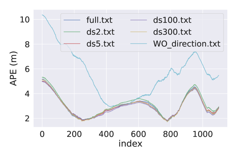

5.4.1 Different Number of Direction Priors
Here we attempt to relax the strength of direction priors by reducing the number of keyframes involved in direction priors. For each direction cluster, downsample at a distance from the distribution of existing VPs. Fig. 6 is a visualization of different downsampled direction priors.Fig. 8 shows the comparison of APE under different .
From those figures, we can concluded that the APE do not suffer drastic expansion due to less direction constraints. Even though there is only about 10 direction constraints retained, we still get quite better accuracy than no direction priors at all. Because the left direction priors can still play some roles. So we argue that as long as there is a few direction constraints over a long distance, the drift will be reduced at a certain level. For each KITTI sequence’s relative rotation error and APE RMSE under differnent , see supplementary material.
We also explore the influence of different scan map size N of each keyframe. The plot and analysis of that result are in supplemental material (page limit).
6 Conclusion
This paper present a strategy that combines map prior and VPs from images to create direction projection error, which is an energy term solely bound on rotation. Then, we implement these direction priors into a visual-LiDAR localization system that tightly couples camera and LiDAR measurements. Experiments on three driving datasets prove that our method achieve lower localization drift. Even though our method is effective and outperforms many related work, There are still two flaws. One thing is time efficiency. Our current implementation can not run in real-time. It is a trade-off between performance and time cost. The second thing is that our method relies on an assumption that agent locally moves on an approximate plane. So compared to UAV or handheld devices, the driving scenes are more likely to meet the above assumptions.
6.0.1 Acknowledgements.
This work is supported by the National Key Research and Development Program of China (2017YFB1002601), National Natural Science Foundation of China (61632003, 61375022, 61403005), Beijing Advanced Innovation Center for Intelligent Robots and Systems (2018IRS11), and PEK-SenseTime Joint Laboratory of Machine Vision.
References
- [1] Andrew, A.M.: Multiple view geometry in computer vision. Kybernetes (2001)
- [2] Barnes, D., Gadd, M., Murcutt, P., Newman, P., Posner, I.: The oxford radar robotcar dataset: A radar extension to the oxford robotcar dataset. In: Proc IEEE Int. Conf. Rob. Autom. (ICRA) (2020). https://doi.org/10.1109/ICRA40945.2020.9196884
- [3] Bosse, M., Rikoski, R., Leonard, J., Teller, S.: Vanishing points and three-dimensional lines from omni-directional video. The Visual Computer 19(6), 417–430 (2003)
- [4] Campos, C., Elvira, R., Rodríguez, J.J.G., Montiel, J.M., Tardós, J.D.: Orb-slam3: An accurate open-source library for visual, visual–inertial, and multimap slam. IEEE Trans. Robot. (2021)
- [5] Chou, C.C., Chou, C.F.: Efficient and accurate tightly-coupled visual-lidar slam. IEEE Trans. Intell. Transp. Syst. (2021)
- [6] Deschaud, J.E.: Imls-slam: scan-to-model matching based on 3d data. In: Proc IEEE Int. Conf. Rob. Autom. (ICRA). pp. 2480–2485. IEEE (2018)
- [7] Geiger, A., Lenz, P., Stiller, C., Urtasun, R.: Vision meets robotics: The kitti dataset. The International Journal of Robotics Research 32(11), 1231–1237 (2013)
- [8] Gräter, J., Wilczynski, A., Lauer, M.: Limo: Lidar-monocular visual odometry. In: Proc IEEE Int. Conf. Intell. Rob. Syst. (IROS). pp. 7872–7879 (2018)
- [9] Grupp, M.: evo: Python package for the evaluation of odometry and slam. https://github.com/MichaelGrupp/evo (2017)
- [10] Huang, S.S., Ma, Z., Mu, T.J., Fu, H., Hu, S.: Lidar-monocular visual odometry using point and line features. In: Proc IEEE Int. Conf. Rob. Autom. (ICRA). pp. 1091–1097 (2020)
- [11] Kümmerle, R., Grisetti, G., Strasdat, H., Konolige, K., Burgard, W.: g 2 o: A general framework for graph optimization. In: Proc IEEE Int. Conf. Rob. Autom. (ICRA). pp. 3607–3613. IEEE (2011)
- [12] Liao, Y., Xie, J., Geiger, A.: KITTI-360: A novel dataset and benchmarks for urban scene understanding in 2d and 3d. arXiv.org 2109.13410 (2021)
- [13] Lim, H., Jeon, J., Myung, H.: Uv-slam: Unconstrained line-based slam using vanishing points for structural mapping. IEEE Robot. Autom. Lett. (2022)
- [14] Lin, J., Zheng, C., Xu, W., Zhang, F.: R2live: A robust, real-time, lidar-inertial-visual tightly-coupled state estimator and mapping. arXiv preprint arXiv:2102.12400 (2021)
- [15] Liu, J., Meng, Z.: Visual slam with drift-free rotation estimation in manhattan world. IEEE Robot. Autom. Lett. 5(4), 6512–6519 (2020)
- [16] Mur-Artal, R., Tardós, J.D.: Orb-slam2: An open-source slam system for monocular, stereo, and rgb-d cameras. IEEE Trans. Robot. 33(5), 1255–1262 (2017)
- [17] Shan, T., Englot, B., Meyers, D., Wang, W., Ratti, C., Rus, D.: Lio-sam: Tightly-coupled lidar inertial odometry via smoothing and mapping. In: Proc IEEE Int. Conf. Intell. Rob. Syst. (IROS). pp. 5135–5142. IEEE (2020)
- [18] Shan, T., Englot, B., Ratti, C., Rus, D.: Lvi-sam: Tightly-coupled lidar-visual-inertial odometry via smoothing and mapping. In: Proc IEEE Int. Conf. Rob. Autom. (ICRA). pp. 5692–5698. IEEE (2021)
- [19] Shin, Y.S., Park, Y.S., Kim, A.: Dvl-slam: sparse depth enhanced direct visual-lidar slam. Auton. Robots 44, 115–130 (2020)
- [20] Sturm, J., Engelhard, N., Endres, F., Burgard, W., Cremers, D.: A benchmark for the evaluation of rgb-d slam systems. In: Proc IEEE Int. Conf. Intell. Rob. Syst. (IROS). pp. 573–580. IEEE (2012)
- [21] Wang, P., Fang, Z., Zhao, S., Chen, Y., Zhou, M., An, S.: Vanishing point aided lidar-visual-inertial estimator. In: Proc IEEE Int. Conf. Rob. Autom. (ICRA). pp. 13120–13126. IEEE (2021)
- [22] Xiang, Z.Z., Yu, J., Li, J., Su, J.: Vilivo: Virtual lidar-visual odometry for an autonomous vehicle with a multi-camera system. In: Proc IEEE Int. Conf. Intell. Rob. Syst. (IROS). pp. 2486–2492 (2019)
- [23] Yu, H., Zhen, W., Yang, W., Zhang, J., Scherer, S.: Monocular camera localization in prior lidar maps with 2d-3d line correspondences. In: Proc IEEE Int. Conf. Intell. Rob. Syst. (IROS). pp. 4588–4594. IEEE (2020)
- [24] Zhang, J., Kaess, M., Singh, S.: A real-time method for depth enhanced visual odometry. Auton. Robots 41(1), 31–43 (2017)
- [25] Zhao, S., Zhang, H., Wang, P., Nogueira, L., Scherer, S.: Super odometry: Imu-centric lidar-visual-inertial estimator for challenging environments. In: Proc IEEE Int. Conf. Intell. Rob. Syst. (IROS). pp. 8729–8736. IEEE (2021)
- [26] Zhen, W., Hu, Y., Yu, H., Scherer, S.: Lidar-enhanced structure-from-motion. In: Proc IEEE Int. Conf. Rob. Autom. (ICRA). pp. 6773–6779 (2020)