Josephson Junction of Nodal Superconductors with Rashba and Ising Spin-Orbit coupling

Transition metal dichalcogenides (TMDs) such as ${\rm NbSe_{2}}$ and ${\rm MoS_{2}}$ have been proposed and experimentally confirmed to be an ideal platform for in-depth explorations for unconventional superconductivity - both intrinsic and externally induced [1, 2, 3, 4, 5, 6, 7, 8, 9, 10, 11, 12, 13, 14].

More recently, cutting-edge advances in fabrication techniques have facilitated the engineering of layered systems from these TMDs where the constituent layers are held together by weak Van der Waals force[15, 16]. Here, some systems are found to retain their superconducting property even down to the monolayer limit [17, 18, 19, 20, 21, 22, 23, 14, 24, 25].

Unlike their bulk counterparts, many monolayer and few-layer TMD’s break inversion symmetry, thereby giving rise to a very strong Ising spin-orbit coupling (SOC) [15, 9, 17, 18, 20, 21, 19, 26, 14] which pins the electron spins perpendicular to the plane. The most remarkable consequence of this strong SOC is that superconductivity survives at high in-plane magnetic fields even beyond the Pauli critical limit [17, 19, 2, 20, 22, 23, 14, 27, 28, 29, 30, 31].

It was proposed that the presence of an in-plane field can induce a topological transition into a nodal superconducting phase [3, 7] protected by a combination of an effective time reversal and particle-hole symmetry. The nodal superconducting phase is expected to be accompanied by Majorana flat bands [32, 33], indication of which have been reported [34, 35], as well as distinct $4\pi$ periodic Josephson current for the transverse momenta in-between the nodal points [36].

In this paper we study the effect of Rashba SOC on the nodal superconducting phase, focusing on the boundary modes and the Josephson current phase relation. Rashba SOC is naturally present due to electronic gates and the presence of a substrate and can be tuned experimentally. The presence of Rashba spin-orbit breaks the chiral symmetry that protects the nodal superconducting phase, and as a result, the nodal points are generally gapped. However, when the in-plane field is aligned along the $\Gamma-K$ direction, a lower crystalline symmetry protects the nodal phase [37]. We study the boundary states in the crystalline phase as well as the current-phase relation in a Josephson-junction geometry. Our results indicate that while the vertical mirror symmetry protects exponentially localized states at the boundary transformed by the symmetry, the current phase relation exhibits a trivial $2\pi$ periodicity in the presence of Rashba spin-orbit.

The plan of the paper is as follows. We begin in Sec. II with an analysis of the low energy momentum-space Hamiltonian and its related symmetries. In Sec. III we introduce a toy model on a triangular lattice which reduces to the continuum Hamiltonian close to the $\Gamma-$ point. We discuss the topological properties of this model with and without Rashba spin-orbit and study the stability of the boundary modes in a ribbon geometry. The physics of a Josephson junction fabricated out of such a material is discussed in Sec. IV.

An Ising superconductor such as monolayer NbSe₂ subjected to an in-plane magnetic field of magnitude $h$, with a superconducting pairing $\Delta$ is governed by the following Bogoliubov-de-Gennes (BdG) Hamiltonian,

	$\displaystyle\cal{H}({\bf k})$	$\displaystyle=$	$\displaystyle\xi({\bf k})\tau^{z}+\lambda({\bf k})\sigma^{z}-\alpha_{R}(k_{x}\tau^{z}\sigma^{y}-k_{y}\sigma^{x})$		(1)
			$\displaystyle+h\cos\theta\tau^{z}\sigma^{x}+h\sin\theta\tau^{0}\sigma^{y}$
			$\displaystyle+\real(\Delta)\tau^{y}\sigma^{y}+\imaginary(\Delta)\tau^{x}\sigma^{y},$

where $\xi({\bf k})=(k_{x}^{2}+k_{y}^{2})/2m-\mu$ is the kinetic energy term with $\mu$ being the chemical potential. The Ising SOC $\lambda({\bf k})=\lambda_{I}(k_{x}^{3}-3k_{x}k_{y}^{2})$ is unique to this class of materials, and pins the electron spins perpendicular to the $x-y$ plane. The form of $\lambda({\bf k})$ is constrained by the crystalline symmetry point group $D_{3h}$ which includes a mirror reflection plane $M_{z}$ (with normal along the $z-$direction), a three-fold rotational symmetry $C_{3}$ and a vertical mirror $M_{x}$ (with normal along the $x-$direction). The strong Ising SOC protects superconductivity in the presence of an in-plane magnetic field $h$ which can exceed the Pauli limit. The parameter $\theta$ denotes the angle the in-plane magnetic field makes with the $x-$axis. $\alpha_{R}$ determines the strength of Rashba SOC, typically present in experimental setups, and can be tuned by gating or by appropriate choice of substrate.

In the absence of Rashba SOC i.e. when $\alpha_{R}=0$, the in-plane direction of $h$ is immaterial. When $|h|>\Delta$ the BdG spectrum has twelve nodal points on the high symmetry $\Gamma-M$ lines $k_{x}=0,\pm\sqrt{3}$ along which the Ising SOC vanishes. This nodal superconducting phase is accompanied by the presence of Majorana flat bands [3, 7, 32, 33], as well as an energy phase relation that depends on the momentum transverse to the current direction, with a $4\pi$ periodicity for the momenta lying between each pair of nodal points [36].

In this work we analyze the effect of Rashba SOC on the nodal superconducting phase, the fate of its boundary modes, and the Josephson current phase relation. To this end, we work in a parameter regime where $h>|\Delta|$ and there are twelve nodal points in the absence of Rashba SOC.

To gain further insight into the topological phase and the nature of its boundary modes, we study a tight-binding model presented in [39, 40] that captures the key features of the topological superconducting phase and exhibits the same low energy physics in the continuum limit $ka\rightarrow 0$.

The lattice model consists of a nearest neighbor hopping:

$\displaystyle H_{0}=-t\sum_{<i,j>,s}{c^{\dagger}_{i,s}}c_{j,s}-\tilde{\mu}\sum_{i,s}{c^{\dagger}_{i,s}}c_{i,s}$

(5)

where $s=\uparrow,\downarrow$ denotes the spin, $<i,j>$ spans all the nearest neighbors and $\tilde{\mu}$ is the on-site chemical potential. In the continuum limit, $ka\rightarrow 0$, this reduces to the kinetic energy term $\xi({\bf k})$ of Eq. (1) when we set $\tilde{\mu}=\mu-6t$ and $t=1/12m$. Similarly, Ising SOC is modeled as a nearest-neighbor hopping with alternating signs (shown in Fig. 1), that reflect the $C_{3}$ symmetry. Note that the sign is opposite for the two spins.

$\displaystyle H_{I}=\frac{i\lambda_{\rm I}}{2}\sum_{<i,j>,s,s^{\prime}}\nu_{ij}\sigma^{z}_{ss^{\prime}}{c^{\dagger}_{i,s}}c_{j,s^{\prime}}$

(6)

where $\nu_{ij}=+1(-1)$ for ${{\bf r}}_{ij}={\bf r}_{i}-{\bf r}_{j}={{\bf a}}_{1},-{{\bf a}}_{2},{{\bf a}}_{2}-{{\bf a}}_{1}(-{{\bf a}}_{1},{{\bf a}}_{2},-{{\bf a}}_{2}+{{\bf a}}_{1})$, respectively, and the lattice vectors are: ${{\bf a}}_{1}=(2a,0)$ and ${{\bf a}}_{2}={a}(1,\sqrt{3})$.

The in-plane magnetic field $({\bf h}=h_{x},h_{y})$

$$H_{B}=\sum_{i,s,s^{\prime}}\left(\bf{h}\cdot\bm{\sigma}\right)_{ss^{\prime}}{c^{\dagger}_{i,s}}{c_{i,s^{\prime}}}$$

(7)

Lastly, the Rashba term can be written as follows

$$H_{R}=-\frac{i\alpha_{R}}{6}\sum_{<i,j>,s,s^{\prime}}{\bf z}\cdot\left({\bf r}_{ij}\times{\bm{\sigma}}\right)_{ss^{\prime}}{c^{\dagger}_{i,s}}{c_{j,s^{\prime}}}$$

(8)

In momentum space the lattice Hamiltonian, eq. (5)-(8) take the following form

	$\displaystyle H$	$\displaystyle=$	$\displaystyle\sum_{{\bf k},s}\tilde{\xi}({\bf k})c_{{\bf k}}^{\dagger}c_{{\bf k}}-\sum_{{\bf k},ss^{\prime}}\tilde{\lambda}_{I}({\bf k})\cdot{\bm{\sigma}}_{ss^{\prime}}c_{{\bf k}s}^{\dagger}c_{{\bf k}s^{\prime}}$
		$\displaystyle+$	$\displaystyle\sum_{{\bf k},ss^{\prime}}\tilde{\alpha}_{R}({\bf k})\cdot{\bm{\sigma}}_{ss^{\prime}}c_{{\bf k}s}^{\dagger}c_{{\bf k}s^{\prime}}+\sum_{{\bf k},ss^{\prime}}{\bf h}\cdot{\bm{\sigma}}_{ss^{\prime}}c_{{\bf k},s}^{\dagger}c_{{\bf k},s^{\prime}},$

where the kinetic energy term is

$$\tilde{\xi}({\bf k})=-4t\cos(k_{x})\cos(\sqrt{3}k_{y})-2t\cos(2k_{x})-\tilde{\mu}.$$

(10)

Here $\tilde{\lambda}_{I}({\bf k})$ and $\tilde{\alpha}_{R}({\bf k})$ correspond to the Ising and Rasbha SOCs respectively and have the following form in the lattice model,

$\displaystyle\tilde{\lambda}_{I}({\bf k})=\lambda_{I}\hat{z}[\sin({\bf k}\cdot{{\bf a}}_{1})+\sin({\bf k}\cdot({{\bf a}}_{2}-{{\bf a}_{1}}))-\sin({\bf k}\cdot{{\bf a}}_{2})],$

and

	$\displaystyle\tilde{\alpha}_{R}({\bf k})$	$\displaystyle=$	$\displaystyle-\frac{\sqrt{3}\alpha_{R}}{2}\hat{x}[\sin({\bf k}\cdot({{\bf a}}_{2}-{{\bf a}_{1}}))+\sin({\bf k}\cdot{{\bf a}}_{2})]$
		$\displaystyle-$	$\displaystyle\frac{\alpha_{R}}{2}\hat{y}[\sin({\bf k}\cdot({{\bf a}}_{2}-{{\bf a}_{1}}))-\sin({\bf k}\cdot{{\bf a}}_{2})-2\sin({\bf k}\cdot{{\bf a}}_{1})]$

The strength of each term is suitably chosen to give the same low energy Hamiltonian as Eq. (1).

Figure 2 shows the dispersion of the two lower energy bands of the lattice model given by Eq. (III), in the vicinity of the $\Gamma$ point. The Rashba SOC breaks the chiral symmetry thus generically lifting the nodal points resulting in a fully gapped phase. However, when the magnetic field is aligned along the $\Gamma-K$ direction, the system has a residual vertical mirror symmetry $M_{x}$, which protects the nodal points along the $k_{x}=0$ symmetry line. The system therefore realizes a nodal crystalline phase, as we show below. Due to the breaking of chiral symmetry, the nodes are shifted away from zero energy.

To study the Josephson energy-phase relation we close the finite ribbon into a torus-like geometry by adding a weak link between the first and last sites of the effective 1D chain, see Fig. 6. All hopping terms across the weak link acquire a phase $\phi$ and are also attenuated by a factor proportional to the strength of the insulating barrier. Varying the phase difference $\phi$ across the junction for a given $k_{y}$ allows to obtain the energy phase relation.

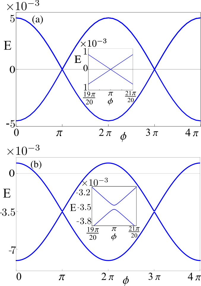
Fig. 7 shows $E(\phi)$ for the mid-gap states at a fixed $k_{y}=0.76$ that lie between pair of nodal points. For $\alpha_{R}=0$ this value of $k_{y}=0.76$ corresponds to a topological non-trivial phase of class BDI with winding $W=1$. Conversely, with $\alpha_{R}\neq 0$ this $k_{y}$ value corresponds to a crystalline topological phase with $\nu_{\cal M}=-1$, see Fig. 3. In the absence of Rashba SOC, shown in Fig. 7 (a), the Josephson energy exhibits a $4\pi$ periodicity similar to the continuous model studied in Ref. 36, with the energy levels crossing zero at $\phi=\pi$ and $3\pi$. This indicates the presence of Majorana edge states localized in the vicinity of the weak link which decay exponentially into the bulk.

When the Rashba SOC is finite, shown in Fig. 7 (b), we find that $E(\phi)$ is no longer symmetric about the $E=0$ line i.e. it is shifted away from zero. Moreover, an energy gap opens at $\phi=\pi,~{}3\pi$ in the presence of a Rashba SOC as is clear from the inset in Fig. 7 (b). Hence, in the presence of Rashba SOC the Josephson energy-phase relation has a $2\pi$ periodicity for all $k_{y}$ values. This is consistent with the observation that the exponentially localized boundary states are not Majorana modes.

We have studied the effect of Rashba spin-orbit coupling on the nodal superconducting phase of an Ising superconductor. This nodal phase was predicted in monolayer TMD’s such as NbSe₂ in the presence of an in-plane field which exceeds the Pauli limit $|h|>\Delta$ [3, 7]. The presence of Rashba SOC breaks the chiral symmetry and generally lifts the nodal points, resulting in a fully gapped state. However, when the magnetic field is aligned along the $\Gamma-K$ line the system has a residual mirror symmetry $M_{x}$ which protects the nodal points at $k_{x}=0$. The system therefore realizes a nodal crystalline phase, characterized by states exponentially localized at the (non-self-reflecting) x-boundary, which disperse parallel to the boundary, provided that the x-boundary preserves the crystalline symmetry. However, we find that even in the presence of exponentially localized boundary states, the current phase relation in a Josephson junction becomes trivial and follows a $2\pi$ periodicity.

We note that Rashba spin-orbit coupling is typically present in experimental setups and can be controlled using gates and by changing substrates. This gives an experimental knob to tune in and out of the topological phase, thus changing the $4\pi$ periodic current phase relation to the trivial $2\pi$.

The authors would like to thank Hadar Steinberg and Ganapathy Murthy for fruitful discussions. D.M. acknowledges support from the Israel Science Foundation (ISF) (grant No. 1884/18). M.K. and D.M. acknowledge support from the ISF, (grant No. 1251/19).

References

- Zhou et al. [2016] B. T. Zhou, N. F. Q. Yuan, H.-L. Jiang, and K. T. Law, Ising superconductivity and majorana fermions in transition-metal dichalcogenides, Physical Review B 93, 180501(R) (2016).
- Ilić et al. [2017] S. Ilić, J. S. Meyer, and M. Houzet, Enhancement of the Upper Critical Field in Disordered Transition Metal Dichalcogenide Monolayers, Physical Review Letters 119, 117001 (2017).
- He et al. [2018] W.-Y. He, B. T. Zhou, J. J. He, N. i. Q. Yuan, T. Zhang, and K. T. Law, Magnetic field driven nodal topological superconductivity in monolayer transition metal dichalcogenides, Communications Physics 1, 40 (2018).
- Sosenko et al. [2017] E. Sosenko, J. Zhang, and V. Aji, Unconventional superconductivity and anomalous response in hole-doped transition metal dichalcogenides, Phys. Rev. B 95, 144508 (2017).
- Nakamura and Yanase [2017] Y. Nakamura and Y. Yanase, Odd-parity superconductivity in bilayer transition metal dichalcogenides, Phys. Rev. B 96, 054501 (2017).
- Möckli and Khodas [2018] D. Möckli and M. Khodas, Robust parity-mixed superconductivity in disordered monolayer transition metal dichalcogenides, Physical Review B 98, 144518 (2018).
- Fischer et al. [2018] M. H. Fischer, M. Sigrist, and D. F. Agterberg, Superconductivity without inversion and time-reversal symmetries, Phys. Rev. Lett. 121, 157003 (2018).
- Smidman et al. [2017a] M. Smidman, M. B. Salamon, H. Q. Yuan, and D. F. Agterberg, Superconductivity and spin-orbit coupling in non-centrosymmetric materials: a review, Reports on Progress in Physics 80, 036501 (2017a).
- Yuan et al. [2014] N. F. Q. Yuan, K. F. Mak, and K. T. Law, Possible topological superconducting phases of , Phys. Rev. Lett. 113, 097001 (2014).
- Oiwa et al. [2018] R. Oiwa, Y. Yanagi, and H. Kusunose, Theory of superconductivity in hole-doped monolayer , Phys. Rev. B 98, 064509 (2018).
- Hsu et al. [2017] Y.-T. Hsu, A. Vaezi, M. H. Fischer, and E.-A. Kim, Topological superconductivity in monolayer transition metal dichalcogenides, Nature Communications 8, 14985 (2017).
- Wang et al. [2018] L. Wang, T. O. Rosdahl, and D. Sticlet, Platform for nodal topological superconductors in monolayer molybdenum dichalcogenides, Phys. Rev. B 98, 205411 (2018).
- Oiwa et al. [2019] R. Oiwa, Y. Yanagi, and H. Kusunose, Time-reversal symmetry breaking superconductivity in hole-doped monolayer mos2, Journal of the Physical Society of Japan 88, 063703 (2019), https://doi.org/10.7566/JPSJ.88.063703 .
- Sohn et al. [2018] E. Sohn, X. Xi, W.-Y. He, S. Jiang, Z. Wang, K. Kang, J.-H. Park, H. Berger, L. Forró, K. T. Law, J. Shan, and K. F. Mak, An unusual continuous paramagnetic-limited superconducting phase transition in 2D NbSe 2, Nature Materials 17, 504 (2018).
- Wang et al. [2012] Q. H. Wang, K. Kalantar-Zadeh, A. Kis, J. N. Coleman, and M. S. Strano, Electronics and optoelectronics of two-dimensional transition metal dichalcogenides, Nature Nanotechnology 7, 699 (2012).
- Geim and Grigorieva [2013] A. K. Geim and I. V. Grigorieva, Van der Waals heterostructures, Nature 499, 419 (2013).
- Lu et al. [2015] J. M. Lu, O. Zheliuk, I. Leermakers, N. F. Q. Yuan, U. Zeitler, K. T. Law, and J. T. Ye, Evidence for two-dimensional Ising superconductivity in gated MoS2, Science 350, 1353 (2015).
- Ugeda et al. [2016] M. M. Ugeda, A. J. Bradley, Y. Zhang, S. Onishi, Y. Chen, W. Ruan, C. Ojeda-Aristizabal, H. Ryu, M. T. Edmonds, H.-Z. Tsai, A. Riss, S.-K. Mo, D. Lee, A. Zettl, Z. Hussain, Z.-X. Shen, and M. F. Crommie, Characterization of collective ground states in single-layer NbSe2, Nature Physics 12, 92 (2016).
- Saito et al. [2016] Y. Saito, Y. Nakamura, M. S. Bahramy, Y. Kohama, J. Ye, Y. Kasahara, Y. Nakagawa, M. Onga, M. Tokunaga, T. Nojima, Y. Yanase, and Y. Iwasa, Superconductivity protected by spin-valley locking in ion-gated mos2, Nature Physics 12, 144 (2016).
- Xi et al. [2016] X. Xi, Z. Wang, W. Zhao, J.-H. Park, K. T. Law, H. Berger, L. Forró, J. Shan, and K. F. Mak, Ising pairing in superconducting nbse2 atomic layers, Nature Physics 12, 139 (2016).
- Costanzo et al. [2016] D. Costanzo, S. Jo, H. Berger, and A. F. Morpurgo, Gate-induced superconductivity in atomically thin mos2 crystals, Nature Nanotechnology 11, 339 (2016).
- Dvir et al. [2018] T. Dvir, F. Massee, L. Attias, M. Khodas, M. Aprili, C. H. L. Quay, and H. Steinberg, Spectroscopy of bulk and few-layer superconducting NbSe2 with van der Waals tunnel junctions, Nature Communications 9, 598 (2018).
- de la Barrera et al. [2018] S. C. de la Barrera, M. R. Sinko, D. P. Gopalan, N. Sivadas, K. L. Seyler, K. Watanabe, T. Taniguchi, A. W. Tsen, X. Xu, D. Xiao, and B. M. Hunt, Tuning ising superconductivity with layer and spin-orbit coupling in two-dimensional transition-metal dichalcogenides, Nature Communications 9, 1427 (2018).
- Xing et al. [2017] Y. Xing, K. Zhao, P. Shan, F. Zheng, Y. Zhang, H. Fu, Y. Liu, M. Tian, C. Xi, H. Liu, J. Feng, X. Lin, S. Ji, X. Chen, Q.-K. Xue, and J. Wang, Ising superconductivity and quantum phase transition in macro-size monolayer nbse2, Nano Letters 17, 6802 (2017).
- Hamill et al. [2021] A. Hamill, B. Heischmidt, E. Sohn, D. Shaffer, K.-T. Tsai, X. Zhang, X. Xi, A. Suslov, H. Berger, L. Forró, F. J. Burnell, J. Shan, K. F. Mak, R. M. Fernandes, K. Wang, and V. S. Pribiag, Two-fold symmetric superconductivity in few-layer nbse2, Nature Physics 10.1038/s41567-021-01219-x (2021).
- Yuan et al. [2016] N. F. Q. Yuan, B. T. Zhou, W.-Y. He, and K. T. Law, Ising superconductivity in transition metal dichalcogenides (2016), arXiv:1605.01847 [cond-mat.supr-con] .
- Liu et al. [2018] Y. Liu, Z. Wang, X. Zhang, C. Liu, Y. Liu, Z. Zhou, J. Wang, Q. Wang, Y. Liu, C. Xi, M. Tian, H. Liu, J. Feng, X. C. Xie, and J. Wang, Interface-Induced Zeeman-Protected Superconductivity in Ultrathin Crystalline Lead Films, Physical Review X 8, 021002 (2018).
- woo Cho et al. [2020] C. woo Cho, J. Lyu, T. Han, C. Y. Ng, Y. Gao, G. Li, M. Huang, N. Wang, J. Schmalian, and R. Lortz, Distinct nodal and nematic superconducting phases in the 2d ising superconductor nbse2 (2020), arXiv:2003.12467 [cond-mat.supr-con] .
- Cho et al. [2022] C.-w. Cho, J. Lyu, L. An, T. Han, K. T. Lo, C. Y. Ng, J. Hu, Y. Gao, G. Li, M. Huang, N. Wang, J. Schmalian, and R. Lortz, Nodal and nematic superconducting phases in monolayers from competing superconducting channels, Phys. Rev. Lett. 129, 087002 (2022).
- Frigeri et al. [2006] P. A. Frigeri, D. F. Agterberg, I. Milat, and M. Sigrist, Phenomenological theory of the s-wave state in superconductors without an inversion center, The European Physical Journal B 54, 435 (2006).
- Kuzmanović et al. [2022] M. Kuzmanović, T. Dvir, D. LeBoeuf, S. Ilić, M. Haim, D. Möckli, S. Kramer, M. Khodas, M. Houzet, J. S. Meyer, M. Aprili, H. Steinberg, and C. H. L. Quay, Tunneling spectroscopy of few-monolayer in high magnetic fields: Triplet superconductivity and ising protection, Phys. Rev. B 106, 184514 (2022).
- Zhao and Wang [2013] Y. X. Zhao and Z. D. Wang, Topological classification and stability of fermi surfaces, Phys. Rev. Lett. 110, 240404 (2013).
- Matsuura et al. [2013] S. Matsuura, P.-Y. Chang, A. P. Schnyder, and S. Ryu, Protected boundary states in gapless topological phases, New Journal of Physics 15, 065001 (2013).
- Galvis et al. [2014] J. A. Galvis, L. Chirolli, I. Guillamón, S. Vieira, E. Navarro-Moratalla, E. Coronado, H. Suderow, and F. Guinea, Zero-bias conductance peak in detached flakes of superconducting 2- probed by scanning tunneling spectroscopy, Phys. Rev. B 89, 224512 (2014).
- Nayak et al. [2021] A. K. Nayak, A. Steinbok, Y. Roet, J. Koo, G. Margalit, I. Feldman, A. Almoalem, A. Kanigel, G. A. Fiete, B. Yan, Y. Oreg, N. Avraham, and H. Beidenkopf, Evidence of topological boundary modes with topological nodal-point superconductivity, Nature Physics 17, 1413 (2021).
- Seshadri et al. [2022] R. Seshadri, M. Khodas, and D. Meidan, Josephson junctions of topological nodal superconductors, SciPost Phys. 12, 197 (2022).
- Shaffer et al. [2020] D. Shaffer, J. Kang, F. J. Burnell, and R. M. Fernandes, Crystalline nodal topological superconductivity and bogolyubov fermi surfaces in monolayer , Phys. Rev. B 101, 224503 (2020).
- Altland and Zirnbauer [1997] A. Altland and M. R. Zirnbauer, Nonstandard symmetry classes in mesoscopic normal-superconducting hybrid structures, Phys. Rev. B 55, 1142 (1997).
- Haim et al. [2022] M. Haim, A. Levchenko, and M. Khodas, Mechanisms of in-plane magnetic anisotropy in superconducting , Phys. Rev. B 105, 024515 (2022).
- Smidman et al. [2017b] M. Smidman, M. Salamon, H. Yuan, and D. Agterberg, Superconductivity and spin–orbit coupling in non-centrosymmetric materials: a review, Reports on Progress in Physics 80, 036501 (2017b).
- Hughes et al. [2011] T. L. Hughes, E. Prodan, and B. A. Bernevig, Inversion-symmetric topological insulators, Phys. Rev. B 83, 245132 (2011).
- Chiu et al. [2013] C.-K. Chiu, H. Yao, and S. Ryu, Classification of topological insulators and superconductors in the presence of reflection symmetry, Phys. Rev. B 88, 075142 (2013).
- Laubscher and Klinovaja [2021] K. Laubscher and J. Klinovaja, Majorana bound states in semiconducting nanostructures, Journal of Applied Physics 130, 081101 (2021), https://doi.org/10.1063/5.0055997 .