JoMA: Demystifying Multilayer Transformers via JOint Dynamics of MLP and Attention
Abstract
We propose Joint MLP/Attention (JoMA) dynamics, a novel mathematical framework to understand the training procedure of multilayer Transformer architectures. This is achieved by integrating out the self-attention layer in Transformers, producing a modified dynamics of MLP layers only. JoMA removes unrealistic assumptions from previous analysis (e.g., lack of residual connection) and predicts that the attention first becomes sparse (to learn salient tokens), then dense (to learn less salient tokens) in the presence of nonlinear activations, while in the linear case, it is consistent with existing works that show attention becomes sparse over time. We leverage JoMA to qualitatively explains how tokens are combined to form hierarchies in multilayer Transformers, when the input tokens are generated by a latent hierarchical generative model. Experiments on models trained from real-world dataset (Wikitext2/Wikitext103) and various pre-trained models (OPT, Pythia) verify our theoretical findings. The code is at111 https://github.com/facebookresearch/luckmatters/tree/yuandong3.
1 Introduction
Since its debut, Transformers (Vaswani et al., 2017) have been extensively used in many applications and demonstrates impressive performance (Dosovitskiy et al., 2020; OpenAI, 2023) compared to domain-specific models (e.g., CNN in computer vision, GNN in graph modeling, RNN/LSTM in language modeling, etc). In all these scenarios, the basic Transformer block, which consists of one self-attention plus two-layer nonlinear MLP, plays a critical role. A natural question arises:
How the basic Transformer block leads to effective learning?
Due to the complexity and nonlinearity of Transformer architectures, it remains a highly nontrivial open problem to find a unified mathematical framework that characterizes the learning mechanism of multi-layer transformers. Existing works mostly focus on 1-layer Transformer (Li et al., 2023a; Tarzanagh et al., 2023b) with fixed MLP (Tarzanagh et al., 2023a) layer, linear activation functions (Tian et al., 2023), and local gradient steps at initialization (Bietti et al., 2023; Oymak et al., 2023), etc.
In this paper, we propose a novel joint dynamics of self-attention plus MLP, based on Joint MLP/Attention Integral (JoMA), a first integral that combines the lower layer of the MLP and self-attention layers. Leveraging this joint dynamics, the self-attention is shown to have more fine-grained and delicate behavior: it first becomes sparse as in the linear case (Tian et al., 2023), only attends to tokens that frequently co-occur with the query, and then becomes denser and gradually includes tokens with less frequent co-occurrence, in the case of nonlinear activation. This shows a changing inductive bias in the Transformer training: first the model focuses on most salient features, then extends to less salient ones.
Another natural question arises: why such a learning pattern is preferred? While for 1-layer this does not give any benefits, in multilayer Transformer setting, we show qualitatively that such a dynamics plays an important role. To demonstrate that this is the case, we assume a hierarchical tree generative model for the input tokens. In this model, starting from the upper level latent variables (in which the top-most is the class label of the input sequence), abbreviated as , generates the latents in the lower layer, until reaching the token level (). With this model, we show that the tokens generated by the lowest latents co-occur a lot and thus can be picked up first by the attention dynamics as “salient features”. This leads to learning of such token combinations in hidden MLP nodes, which triggers self-attention grouping at , etc. In this way, the non-salient co-occurrences are naturally explained by the top level hierarchy, rather than incorrectly learned by the lower layer as spurious correlation, which is fortunately delayed by the attention mechanism. Our theoretical finding is consistent with both the pre-trained models such as OPT/Pythia and models trained from scratch using real-world dataset (Wikitext2 and Wikitext103).
We show that JoMA overcomes several main limitations from Scan&Snap (Tian et al., 2023). JoMA incorporates residual connections and MLP nonlinearity as key ingredients, analyzes joint training of MLP and self-attention layer, and qualitatively explains dynamics of multilayer Transformers. For linear activation, JoMA coincides with Scan&Snap, i.e., the attention becomes sparse during training.
1.1 Related Work
Expressiveness of Attention-based Models. The universal approximation abilities of attention-based models have been studied extensively (Yun et al., 2019; Bhattamishra et al., 2020a; b; Dehghani et al., 2018; Pérez et al., 2021). More recent studies offer detailed insights into their expressiveness for specific functions across various scenarios, sometimes incorporating statistical evaluations (Edelman et al., 2022; Elhage et al., 2021; Likhosherstov et al., 2021; Akyürek et al., 2022; Zhao et al., 2023; Yao et al., 2021; Anil et al., 2022; Barak et al., 2022). A fruitful line of work studied in-context learning capabilities of the Transformer (Dong et al., 2022), linking gradient descent in classification/regression learning to the feedforward actions in Transformer layers (Garg et al., 2022; Von Oswald et al., 2022; Bai et al., 2023; Olsson et al., 2022; Akyürek et al., 2022; Li et al., 2023b). However, unlike our study, these work do not characterize the training dynamics.
Training Dynamics of Neural Networks. Earlier research has delved into training dynamics within multi-layer linear neural networks (Arora et al., 2018; Bartlett et al., 2018), the teacher-student setting (Brutzkus & Globerson, 2017; Tian, 2017; Soltanolkotabi, 2017; Goel et al., 2018; Du et al., 2017; 2018a; Zhou et al., 2019; Liu et al., 2019; Xu & Du, 2023), and infinite-width limits (Jacot et al., 2018; Chizat et al., 2019; Du et al., 2018b; 2019; Allen-Zhu et al., 2019; Arora et al., 2019; Oymak & Soltanolkotabi, 2020; Zou et al., 2020; Li & Liang, 2018; Chizat & Bach, 2018; Mei et al., 2018; Nguyen & Pham, 2020; Fang et al., 2021; Lu et al., 2020). This includes extensions to attention-based-models (Hron et al., 2020; Yang et al., 2022). For self-supervised learning, there are analyses of linear networks (Tian, 2022) and explorations into the impact of nonlinearity (Tian, 2023).
Dynamics of Attention-based models. Regarding attention-based models, Zhang et al. (2020) delves into adaptive optimization techniques. Jelassi et al. (2022) introduces an idealized context, demonstrating that the vision transformer (Dosovitskiy et al., 2020) trained via gradient descent can discern spatial structures. Li et al. (2023c) illustrates that a single-layer Transformer can learn a constrained topic model, where each word is tied to a single topic, using loss, BERT-like framework (Devlin et al., 2018), and certain assumptions on attention patterns. Snell et al. (2021) investigate the training dynamics of single-head attention in mimicking Seq2Seq learning. Tian et al. (2023) characterizes the SGD training dynamics of a 1-layer Transformer and shows that with cross-entropy loss, the model will pay more attention to the key tokens that frequently co-occur with the query token. Oymak et al. (2023) constructs the attention-based contextual mixture model and demonstrates how the prompt can attend to the sparse context-relevant tokens via gradient descent. Tarzanagh et al. (2023b) also finds that running gradient descent will converge in direction to the max-margin solution that separates the locally optimal tokens from others, and Tarzanagh et al. (2023a) further disclose the connection between the optimization geometry of self-attention and hard-margin SVM problem. For the in-context learning scenario, several recent works analyze linear transformers trained on random instances for linear regression tasks from the perspective of loss landscape (Boix-Adsera et al., 2023; Zhang et al., 2023). While these studies also study the optimization dynamics of attention-based models, they do not reveal the phenomena we discuss.
2 Problem Setting
Let the total vocabulary size be , in which is the number of contextual tokens and is the number of query tokens. Consider one layer in multilayer transformer (Fig. 1(b)):
| (1) |
Input/outputs. is the input frequency vector for contextual token , is the query token index, is the number of nodes in the hidden MLP layer, whose outputs are . All the quantities above vary across different sample index (i.e., , ). In addition, is the nonlinearity (e.g., ReLU).
Model weights. is the (unnormalized) attention logits given query , and are the weights for the lower MLP layer. These will be analyzed in the paper.

The Attention Mechanism. In this paper, we mainly study three kinds of attention:
-
•
Linear Attention (Von Oswald et al., 2022): and ;
-
•
Exp Attention: and ;
-
•
Softmax Attention (Vaswani et al., 2017): and .
Here is the Hadamard (element-wise) product. are the attention scores for contextual tokens, given by a point-wise attention function . is the normalization constant.
Embedding vectors. is the embedding vector for token . We assume that the embedding dimension is sufficiently large and thus , i.e., are orthonormal bases. Let be the matrix that encodes all embedding vectors of contextual tokens. Then . Appendix B.1 verifies the orthogonality assumption in multiple pre-trained models (Pythia, LLaMA, etc).
Residual connections are introduced as an additional term in Eqn. 1, which captures the critical component in Transformer architecture. Note that we do not model value matrix since it can be merged into the embedding vectors (e.g., by ), while and are already implicitly modeled by the self-attention logits .
Gradient backpropagation in multilayers. In multilayer setting, the gradient gets backpropagated from top layer. Specifically, let be the backpropagated gradient sent to node at sample . For 1-layer Transformer with softmax loss directly applied to the hidden nodes of MLP, we have , where is the label to be predicted for sample . For brevity, we often omit sample index if there is no ambiguity.
Assumption 1 (Stationary backpropagated gradient ).
Expectation terms involving (e.g., ) remains constant during training.
Note that this is true for layer-wise training: optimizing the weights for a specific Transformer layer, while fixing the weights of others and thus the statistics of backpropagated are stationary. For joint training, this condition also holds approximately since the weights change gradually during the training process. Under Assumption 1, Appendix A.1 gives an equivalent formulation in terms of per-hidden node loss.
Training Dynamics. Define the conditional expectation . Now let us consider the dynamics of and , if we train the model with a batch of inputs that always end up with query , then:
| (2) |
Here is the derivative of current activation and .

3 JoMA: Existence of JOint dynamics of Attention and MLP
While the learning dynamics of and can be complicated, surprisingly, training dynamics suggests that the attention logits have close-form relationship with respect to the MLP weights , which lays the foundation of our JoMA framework:
Theorem 1 (JoMA).
Let , then the dynamics of Eqn. 2 satisfies the invariants:
-
•
Linear attention. The dynamics satisfies .
-
•
Exp attention. The dynamics satisfies .
-
•
Softmax attention. If is a constant over time and , then the dynamics satisfies .
Under zero initialization (, ), then the time-independent constant .
Therefore, we don’t need to explicitly update self-attention, since it is already implicitly incorporated in the lower layer of MLP weight! For softmax attention, we verify that even with the assumption, the invariance proposed by Theorem 1 still predicts fairly well.
3.1 Linear activations: winner-take-all
Now we can solve the dynamics of (Eqn. 2), by plugging in the close-form solution of self-attention. For simplicity, we consider exp attention with (i.e., single hidden MLP node). Let , then ’s dynamics is ( written as ):
| (3) |
In the case of linear activations , . According to Assumption 1, does not depend on and we arrive at the following theorem:

Theorem 2 (Linear Dynamics with Self-attention).
With linear MLP activation and zero initialization, for exp attention any two tokens satisfy the following invariants:
| (4) |
where and is Gauss error function.
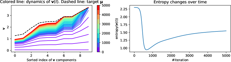
Remarks. The dynamics suggests that the weights become one-hot over training. Specifically, let , then and other converges to finite numbers, because of the constraint imposed by Eqn. 4 (see Fig. 3). For softmax attention, there is an additional sample-dependent normalization constant , if remains constant across samples and all elements of are the same, then Theorem 2 also applies.
Beyond distinct/common tokens. 222Since is the empirical frequency of token in sample , we have . is a product of token discriminancy (i.e., means token positively correlated to backpropagated gradient , or label in the 1-layer case) and token frequency (i.e., , how frequent appears given ). This covers a broader spectrum of tokens than Tian et al. (2023), which only discusses distinct (i.e., large ) and common tokens (i.e., when ).
4 Training Dynamics under Nonlinear Activations
In nonlinear case, the dynamics turns out to be very different. In this case, is no longer a constant, but will change. As a result, the dynamics also changes substantially.
Theorem 3 (Dynamics of nonlinear activation with uniform attention).
If is sampled from a mixture of isotropic distributions centered at , where each and gradient are constant within each mixture, then:
| (5) |
here , is the affinity to and the “bias” term , and depend on derivative of nonlinearity and data distribution but not . If is monotonous with and , so does .
Appendix A.3.2 presents critical point analysis. Here we focus on a simplified one when is constrained to be a unit vector, which leads to the following modified dynamics ():
| (6) |
where . We consider when is aligned with one cluster but far away from others, then for and since is monotonously increasing. Hence dominates and let for brevity. Similar to Eqn. 3, we use close-form simplification of JoMA to incorporate self-attention, which leads to (we use exp attention):
| (7) |
Here we omit the scalar terms and study when is close to , in which . It is clear that the critical point does not change after adding the term . However, the convergence speed changes drastically. As shown in the following lemma, the convergence speed towards salient component of (i.e., component with large magnitude) is much faster than non-salient ones:
Theorem 4 (Convergence speed of salient vs. non-salient components).
Let be the convergence metric for component ( means that the component converges). For nonlinear dynamics with attention (Eqn. 7), then
| (8) |
Here where and only depends on and . So when , we have .
Remarks. For linear attention, the ratio is different but the derivation is similar and simpler. Note that the convergence speed heavily depends on the magnitude of . If , then and converges much faster than . Therefore, the salient (i.e., large) components is learned first, and the non-salient (i.e., small) component is learned later, due to the modulation of the extra term thanks to self-attention, as demonstrated in Fig. 4.
A follow-up question arises: What is the intuition behind salient and non-salient components in ? Note that is an -normalized version of the conditional token frequency , given the query . In this case, similar to Theorem 2 (and Tian et al. (2023)), we again see that if a contextual token co-occurs a lot with the query , then the corresponding component becomes larger and the growth speed of towards is much faster.
Relationship with rank of MLP lower layer. Since MLP and attention layer has joint dynamics (Theorem 1), this also suggests that in the MLP layer, the rank of lower layer matrix (which projects into the hidden nodes) will first drop since the weight components that correspond to high target value grow first, and then bounce back to higher rank when the components that correspond to low target value catch up later.
5 How self-attention learns hierarchical data distribution?
A critical difference between the training dynamics of linear and nonlinear MLP is that in the nonlinear case, although slowly, the non-salient components will still grow, and the entropy of the attention bounces back later. While for 1-layer Transformer, this may only slow the training with no clear benefits, the importance of such a behavior is manifested if we think about the dynamics of multiple Transformer layers trained on a data distribution generated in a hierarchical manner.
Consider a simple generative hierarchical binary latent tree model (HBLT) (Tian et al., 2020) (Fig. 7(a)) in which we have latent (unobservable) binary variables at layer that generate latents at layer , until the observable tokens are generated at the lowest level (). The topmost layer is the class label , which can take discrete values. In HBLT, the generation process of at layer given at layer can be characterized by their conditional probability . The uncertainty hyperparameter determines how much the top level latents can determine the values of the low level ones. Please check Appendix A.5 for its formal definition.
With HBLT, we can compute the co-occurrence frequency of two tokens and , as a function of the depth of their common latent ancestor (CLA):
Theorem 5 (Token Co-occurrence in ).
If token and have common latent ancestor (CLA) of depth (Fig. 5(c)), then , where is the total depth of the hierarchy and , in which and , where are the immediate children of the root node .
Remarks. If takes multiple values (many classes) and each class only trigger one specific latent binary variables, then most of the top layer latents are very sparsely triggered and thus is very close to . If is also close to , then for deep hierarchy and shallow common ancestor, . To see this, assume , then we have:
| (9) |
This means that two tokens and co-occur a lot, if they have a shallow CLA ( small) that is close to both tokens. If their CLA is high in the hierarchy (e.g., and ), then the token and have much weaker co-occurrence and (and thus and ) is small.

With this generative model, we can analyze qualitatively the learning dynamics of JoMA: first it focuses on associating the tokens in the same lowest hierarchy as the query (and these tokens co-occur a lot with ), then gradually reaches out to other tokens that co-occur less with , if they have not been picked up by other tokens (Fig. 5(b)); if co-occurs a lot with some other , then - and - form their own lower hierarchy, respectively. This leads to learning of high-level features and , which has high correlation are associated in the higher level. Therefore, the latent hierarchy is implicitly learned.
6 Experiments
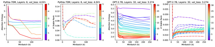
Dynamics of Attention Sparsity. Fig. 6 shows how attention sparsity changes over time when training from scratch. We use learning rate and test our hypothesis on Wikitext2/Wikitext103 (Merity et al., 2016) (top/bottom row). Fig. 8 further shows that different learning rate leads to different attention sparsity patterns. With large learning rate, attention becomes extremely sparse as in (Tian et al., 2023). Interestingly, the attention patterns, which coincide with our theoretical analysis, yield the best validation score.
We also tested our hypothesis in OPT (Zhang et al., 2022) (OPT-2.7B) and Pythia (Biderman et al., 2023) (Pythia-70M/1.4B/6.9B) pre-trained models, both of which has public intermediate checkpoints. While the attention patterns show less salient drop-and-bounce patterns, the dynamics of stable ranks of the MLP lower layer (projection into hidden neurons) show much salient such structures for top layers, and dropping curves for bottom layers since they are suppressed by top-level learning (Sec. 5). Note that stable ranks only depend on the model parameters and thus may be more reliable than attention sparsity.


Validation of Alignment between latents and hidden nodes in MLP. Sec. 5 is based on an assumption that the hidden nodes in MLP layer will learn the latent variables. We verify this assumption in synthetic data sampled by HBLT, which generate latent variables in a top-down manner, until the final tokens are generated. The latent hierarchy has 2 hyperparameters: number of latents per layer () and number of children per latent (). is the number of classes. Adam optimizer is used with learning rate . Vocabulary size , sequence length and embedding dimension .
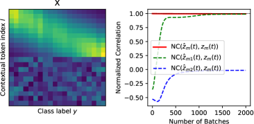
We use 3-layer generative model as well as 3-layer Transformer models. We indeed perceive high correlations between the latents and the hidden neurons between corresponding layers. Note that latents are known during input generation procedure but are not known to the transformer being trained. We take the maximal activation of each neuron across the sequence length, and compute normalized correlation between maximal activation of each neuron and latents, after centeralizing across the sample dimension. Tbl. 1 shows that indeed in the learned models, for each latent, there exists at least one hidden node in MLP that has high normalized correlation with it, in particular in the lowest layer. When the generative models becomes more complicated (i.e., both and become larger), the correlation goes down a bit.
| , | , | , | ||||
|---|---|---|---|---|---|---|
| (10, 20) | (20, 30) | (10, 20) | (20, 30) | (10, 20) | (20, 30) | |
| NCorr () | ||||||
| NCorr () | ||||||
| , | , | |||||
| (10, 20) | (20, 30) | (10, 20) | (20, 30) | (10, 20) | (20, 30) | |
| NCorr () | ||||||
| NCorr () | ||||||
7 Discussion
Deal with almost orthogonal embeddings. In this paper, we focus on fixed orthonormal embeddings vectors. However, in real-world Transformer training, the assumption may not be valid, since often the embedding dimension is smaller than the number of vocabulary so the embedding vectors cannot be orthogonal to each other. In this setting, one reasonable assumption is that the embedding vectors are almost orthogonal. Thanks to Johnson–Lindenstrauss lemma, one interesting property of high-dimensional space is that for embedding vectors to achieve almost orthogonality , only is needed. As a result, our JoMA framework (Theorem 1) will have additional -related terms and we leave the detailed analysis as one of our future work.
Training embedding vectors. Another factor that is not considered in JoMA is that the embedding vectors are also trained simultaneously. This could further boost the efficiency of Transformer architecture, since concepts with similar semantics will learn similar embeddings. This essentially reduces the vocabulary size at each layer for learning to be more effective, and leads to better generalization. For example, in each hidden layer hidden neurons are computed, which does not mean there are independent intermediate “tokens”, because many of their embeddings are highly correlated.
Self-attention computed from embedding. JoMA arrives at the joint dynamics of MLP and attention by assuming that the pairwise attention score is an independent parameters optimized under SGD dynamics. In practice, is also parameterized by the embedding matrix, which allow generalization to tokens with similar embeddings, and may accelerate the training dynamics of . We leave it in the future works.
8 Conclusion
We propose JoMA, a framework that characterizes the joint training dynamics of nonlinear MLP and attention layer, by integrating out the self-attention logits. The resulting dynamics connects the dynamics of nonlinear MLP lower layer weights (projection into hidden neurons) and self-attention, and shows that the attention first becomes sparse (or weights becomes low rank) and then becomes dense (or weights becomes high rank). Furthermore, we qualitatively give a learning mechanism of multilayer Transformer that reveals how self-attentions at different layers interact with each other to learn the latent feature hierarchy.
Acknowledgments
Simon S. Du is supported by supported by NSF IIS 2110170, NSF DMS 2134106, NSF CCF 2212261, NSF IIS 2143493, NSF CCF 2019844, NSF IIS 2229881.
References
- Akyürek et al. (2022) Ekin Akyürek, Dale Schuurmans, Jacob Andreas, Tengyu Ma, and Denny Zhou. What learning algorithm is in-context learning? investigations with linear models. arXiv preprint arXiv:2211.15661, 2022.
- Allen-Zhu et al. (2019) Zeyuan Allen-Zhu, Yuanzhi Li, and Zhao Song. A convergence theory for deep learning via over-parameterization. In International Conference on Machine Learning, pp. 242–252. PMLR, 2019.
- Anil et al. (2022) Cem Anil, Yuhuai Wu, Anders Andreassen, Aitor Lewkowycz, Vedant Misra, Vinay Ramasesh, Ambrose Slone, Guy Gur-Ari, Ethan Dyer, and Behnam Neyshabur. Exploring length generalization in large language models. arXiv preprint arXiv:2207.04901, 2022.
- Arora et al. (2018) Sanjeev Arora, Nadav Cohen, Noah Golowich, and Wei Hu. A convergence analysis of gradient descent for deep linear neural networks. arXiv preprint arXiv:1810.02281, 2018.
- Arora et al. (2019) Sanjeev Arora, Simon Du, Wei Hu, Zhiyuan Li, and Ruosong Wang. Fine-grained analysis of optimization and generalization for overparameterized two-layer neural networks. In International Conference on Machine Learning, pp. 322–332. PMLR, 2019.
- Bai et al. (2023) Yu Bai, Fan Chen, Huan Wang, Caiming Xiong, and Song Mei. Transformers as statisticians: Provable in-context learning with in-context algorithm selection. arXiv preprint arXiv:2306.04637, 2023.
- Barak et al. (2022) Boaz Barak, Benjamin Edelman, Surbhi Goel, Sham Kakade, Eran Malach, and Cyril Zhang. Hidden progress in deep learning: Sgd learns parities near the computational limit. Advances in Neural Information Processing Systems, 35:21750–21764, 2022.
- Bartlett et al. (2018) Peter Bartlett, Dave Helmbold, and Philip Long. Gradient descent with identity initialization efficiently learns positive definite linear transformations by deep residual networks. In International conference on machine learning, pp. 521–530. PMLR, 2018.
- Bhattamishra et al. (2020a) Satwik Bhattamishra, Kabir Ahuja, and Navin Goyal. On the ability and limitations of transformers to recognize formal languages. arXiv preprint arXiv:2009.11264, 2020a.
- Bhattamishra et al. (2020b) Satwik Bhattamishra, Arkil Patel, and Navin Goyal. On the computational power of transformers and its implications in sequence modeling. arXiv preprint arXiv:2006.09286, 2020b.
- Biderman et al. (2023) Stella Biderman, Hailey Schoelkopf, Quentin Gregory Anthony, Herbie Bradley, Kyle O’Brien, Eric Hallahan, Mohammad Aflah Khan, Shivanshu Purohit, USVSN Sai Prashanth, Edward Raff, et al. Pythia: A suite for analyzing large language models across training and scaling. In International Conference on Machine Learning, pp. 2397–2430. PMLR, 2023.
- Bietti et al. (2023) Alberto Bietti, Vivien Cabannes, Diane Bouchacourt, Herve Jegou, and Leon Bottou. Birth of a transformer: A memory viewpoint. arXiv preprint arXiv:2306.00802, 2023.
- Boix-Adsera et al. (2023) Enric Boix-Adsera, Etai Littwin, Emmanuel Abbe, Samy Bengio, and Joshua Susskind. Transformers learn through gradual rank increase. arXiv preprint arXiv:2306.07042, 2023.
- Brutzkus & Globerson (2017) Alon Brutzkus and Amir Globerson. Globally optimal gradient descent for a convnet with gaussian inputs. In International conference on machine learning, pp. 605–614. PMLR, 2017.
- Chizat & Bach (2018) Lenaic Chizat and Francis Bach. On the global convergence of gradient descent for over-parameterized models using optimal transport. Advances in neural information processing systems, 31, 2018.
- Chizat et al. (2019) Lenaic Chizat, Edouard Oyallon, and Francis Bach. On lazy training in differentiable programming. Advances in neural information processing systems, 32, 2019.
- Dehghani et al. (2018) Mostafa Dehghani, Stephan Gouws, Oriol Vinyals, Jakob Uszkoreit, and Łukasz Kaiser. Universal transformers. arXiv preprint arXiv:1807.03819, 2018.
- Devlin et al. (2018) Jacob Devlin, Ming-Wei Chang, Kenton Lee, and Kristina Toutanova. Bert: Pre-training of deep bidirectional transformers for language understanding. arXiv preprint arXiv:1810.04805, 2018.
- Dong et al. (2022) Qingxiu Dong, Lei Li, Damai Dai, Ce Zheng, Zhiyong Wu, Baobao Chang, Xu Sun, Jingjing Xu, and Zhifang Sui. A survey for in-context learning. arXiv preprint arXiv:2301.00234, 2022.
- Dosovitskiy et al. (2020) Alexey Dosovitskiy, Lucas Beyer, Alexander Kolesnikov, Dirk Weissenborn, Xiaohua Zhai, Thomas Unterthiner, Mostafa Dehghani, Matthias Minderer, Georg Heigold, Sylvain Gelly, et al. An image is worth 16x16 words: Transformers for image recognition at scale. arXiv preprint arXiv:2010.11929, 2020.
- Du et al. (2018a) Simon Du, Jason Lee, Yuandong Tian, Aarti Singh, and Barnabas Poczos. Gradient descent learns one-hidden-layer cnn: Don’t be afraid of spurious local minima. In International Conference on Machine Learning, pp. 1339–1348. PMLR, 2018a.
- Du et al. (2019) Simon Du, Jason Lee, Haochuan Li, Liwei Wang, and Xiyu Zhai. Gradient descent finds global minima of deep neural networks. In International conference on machine learning, pp. 1675–1685. PMLR, 2019.
- Du et al. (2017) Simon S Du, Jason D Lee, and Yuandong Tian. When is a convolutional filter easy to learn? arXiv preprint arXiv:1709.06129, 2017.
- Du et al. (2018b) Simon S. Du, Xiyu Zhai, Barnabas Poczos, and Aarti Singh. Gradient descent provably optimizes over-parameterized neural networks, 2018b. URL https://arxiv.org/abs/1810.02054.
- Edelman et al. (2022) Benjamin L Edelman, Surbhi Goel, Sham Kakade, and Cyril Zhang. Inductive biases and variable creation in self-attention mechanisms. In International Conference on Machine Learning, pp. 5793–5831. PMLR, 2022.
- Elhage et al. (2021) N Elhage, N Nanda, C Olsson, T Henighan, N Joseph, B Mann, A Askell, Y Bai, A Chen, T Conerly, et al. A mathematical framework for transformer circuits. Transformer Circuits Thread, 2021.
- Fang et al. (2021) Cong Fang, Jason Lee, Pengkun Yang, and Tong Zhang. Modeling from features: a mean-field framework for over-parameterized deep neural networks. In Conference on learning theory, pp. 1887–1936. PMLR, 2021.
- Garg et al. (2022) Shivam Garg, Dimitris Tsipras, Percy S Liang, and Gregory Valiant. What can transformers learn in-context? a case study of simple function classes. Advances in Neural Information Processing Systems, 35:30583–30598, 2022.
- Goel et al. (2018) Surbhi Goel, Adam Klivans, and Raghu Meka. Learning one convolutional layer with overlapping patches. In International Conference on Machine Learning, pp. 1783–1791. PMLR, 2018.
- Hron et al. (2020) Jiri Hron, Yasaman Bahri, Jascha Sohl-Dickstein, and Roman Novak. Infinite attention: Nngp and ntk for deep attention networks. In International Conference on Machine Learning, pp. 4376–4386. PMLR, 2020.
- Jacot et al. (2018) Arthur Jacot, Franck Gabriel, and Clément Hongler. Neural tangent kernel: Convergence and generalization in neural networks. Advances in neural information processing systems, 31, 2018.
- Jelassi et al. (2022) Samy Jelassi, Michael Sander, and Yuanzhi Li. Vision transformers provably learn spatial structure. Advances in Neural Information Processing Systems, 35:37822–37836, 2022.
- Li et al. (2023a) Hongkang Li, Meng Wang, Sijia Liu, and Pin-Yu Chen. A theoretical understanding of shallow vision transformers: Learning, generalization, and sample complexity. In The Eleventh International Conference on Learning Representations, 2023a. URL https://openreview.net/forum?id=jClGv3Qjhb.
- Li et al. (2023b) Shuai Li, Zhao Song, Yu Xia, Tong Yu, and Tianyi Zhou. The closeness of in-context learning and weight shifting for softmax regression. arXiv preprint arXiv:2304.13276, 2023b.
- Li & Liang (2018) Yuanzhi Li and Yingyu Liang. Learning overparameterized neural networks via stochastic gradient descent on structured data. Advances in neural information processing systems, 31, 2018.
- Li et al. (2023c) Yuchen Li, Yuanzhi Li, and Andrej Risteski. How do transformers learn topic structure: Towards a mechanistic understanding. arXiv preprint arXiv:2303.04245, 2023c.
- Likhosherstov et al. (2021) Valerii Likhosherstov, Krzysztof Choromanski, and Adrian Weller. On the expressive power of self-attention matrices. arXiv preprint arXiv:2106.03764, 2021.
- Liu et al. (2019) Tianyi Liu, Minshuo Chen, Mo Zhou, Simon S Du, Enlu Zhou, and Tuo Zhao. Towards understanding the importance of shortcut connections in residual networks. Advances in neural information processing systems, 32, 2019.
- Lu et al. (2020) Yiping Lu, Chao Ma, Yulong Lu, Jianfeng Lu, and Lexing Ying. A mean field analysis of deep resnet and beyond: Towards provably optimization via overparameterization from depth. In International Conference on Machine Learning, pp. 6426–6436. PMLR, 2020.
- Mei et al. (2018) Song Mei, Andrea Montanari, and Phan-Minh Nguyen. A mean field view of the landscape of two-layer neural networks. Proceedings of the National Academy of Sciences, 115(33):E7665–E7671, 2018.
- Merity et al. (2016) Stephen Merity, Caiming Xiong, James Bradbury, and Richard Socher. Pointer sentinel mixture models. arXiv preprint arXiv:1609.07843, 2016.
- Nguyen & Pham (2020) Phan-Minh Nguyen and Huy Tuan Pham. A rigorous framework for the mean field limit of multilayer neural networks. arXiv preprint arXiv:2001.11443, 2020.
- Olsson et al. (2022) Catherine Olsson, Nelson Elhage, Neel Nanda, Nicholas Joseph, Nova DasSarma, Tom Henighan, Ben Mann, Amanda Askell, Yuntao Bai, Anna Chen, et al. In-context learning and induction heads. arXiv preprint arXiv:2209.11895, 2022.
- OpenAI (2023) OpenAI. Gpt-4 technical report, 2023.
- Oymak & Soltanolkotabi (2020) Samet Oymak and Mahdi Soltanolkotabi. Toward moderate overparameterization: Global convergence guarantees for training shallow neural networks. IEEE Journal on Selected Areas in Information Theory, 1(1):84–105, 2020.
- Oymak et al. (2023) Samet Oymak, Ankit Singh Rawat, Mahdi Soltanolkotabi, and Christos Thrampoulidis. On the role of attention in prompt-tuning. ICML, 2023.
- Pérez et al. (2021) Jorge Pérez, Pablo Barceló, and Javier Marinkovic. Attention is turing complete. The Journal of Machine Learning Research, 22(1):3463–3497, 2021.
- Snell et al. (2021) Charlie Snell, Ruiqi Zhong, Dan Klein, and Jacob Steinhardt. Approximating how single head attention learns. arXiv preprint arXiv:2103.07601, 2021.
- Soltanolkotabi (2017) Mahdi Soltanolkotabi. Learning relus via gradient descent. Advances in neural information processing systems, 30, 2017.
- Tarzanagh et al. (2023a) Davoud Ataee Tarzanagh, Yingcong Li, Christos Thrampoulidis, and Samet Oymak. Transformers as support vector machines. arXiv preprint arXiv:2308.16898, 2023a.
- Tarzanagh et al. (2023b) Davoud Ataee Tarzanagh, Yingcong Li, Xuechen Zhang, and Samet Oymak. Max-margin token selection in attention mechanism. arXiv preprint arXiv:2306.13596, 3(7):47, 2023b.
- Tian (2017) Yuandong Tian. An analytical formula of population gradient for two-layered relu network and its applications in convergence and critical point analysis. In International conference on machine learning, pp. 3404–3413. PMLR, 2017.
- Tian (2022) Yuandong Tian. Understanding the role of nonlinearity in training dynamics of contrastive learning. arXiv preprint arXiv:2206.01342, 2022.
- Tian (2023) Yuandong Tian. Understanding the role of nonlinearity in training dynamics of contrastive learning. ICLR, 2023.
- Tian et al. (2020) Yuandong Tian, Lantao Yu, Xinlei Chen, and Surya Ganguli. Understanding self-supervised learning with dual deep networks. arXiv preprint arXiv:2010.00578, 2020.
- Tian et al. (2023) Yuandong Tian, Yiping Wang, Beidi Chen, and Simon Du. Scan and snap: Understanding training dynamics and token composition in 1-layer transformer, 2023.
- Vaswani et al. (2017) Ashish Vaswani, Noam Shazeer, Niki Parmar, Jakob Uszkoreit, Llion Jones, Aidan N. Gomez, Lukasz Kaiser, and Illia Polosukhin. Attention is all you need. 2017. URL https://arxiv.org/pdf/1706.03762.pdf.
- Von Oswald et al. (2022) Johannes Von Oswald, Eyvind Niklasson, Ettore Randazzo, João Sacramento, Alexander Mordvintsev, Andrey Zhmoginov, and Max Vladymyrov. Transformers learn in-context by gradient descent. arXiv preprint arXiv:2212.07677, 2022.
- Xu & Du (2023) Weihang Xu and Simon S Du. Over-parameterization exponentially slows down gradient descent for learning a single neuron. arXiv preprint arXiv:2302.10034, 2023.
- Yang et al. (2022) Greg Yang, Edward J Hu, Igor Babuschkin, Szymon Sidor, Xiaodong Liu, David Farhi, Nick Ryder, Jakub Pachocki, Weizhu Chen, and Jianfeng Gao. Tensor programs v: Tuning large neural networks via zero-shot hyperparameter transfer. arXiv preprint arXiv:2203.03466, 2022.
- Yao et al. (2021) Shunyu Yao, Binghui Peng, Christos Papadimitriou, and Karthik Narasimhan. Self-attention networks can process bounded hierarchical languages. arXiv preprint arXiv:2105.11115, 2021.
- Yun et al. (2019) Chulhee Yun, Srinadh Bhojanapalli, Ankit Singh Rawat, Sashank J Reddi, and Sanjiv Kumar. Are transformers universal approximators of sequence-to-sequence functions? arXiv preprint arXiv:1912.10077, 2019.
- Zhang et al. (2020) Jingzhao Zhang, Sai Praneeth Karimireddy, Andreas Veit, Seungyeon Kim, Sashank Reddi, Sanjiv Kumar, and Suvrit Sra. Why are adaptive methods good for attention models? Advances in Neural Information Processing Systems, 33:15383–15393, 2020.
- Zhang et al. (2023) Ruiqi Zhang, Spencer Frei, and Peter L Bartlett. Trained transformers learn linear models in-context. arXiv preprint arXiv:2306.09927, 2023.
- Zhang et al. (2022) Susan Zhang, Stephen Roller, Naman Goyal, Mikel Artetxe, Moya Chen, Shuohui Chen, Christopher Dewan, Mona Diab, Xian Li, Xi Victoria Lin, et al. Opt: Open pre-trained transformer language models. arXiv preprint arXiv:2205.01068, 2022.
- Zhao et al. (2023) Haoyu Zhao, Abhishek Panigrahi, Rong Ge, and Sanjeev Arora. Do transformers parse while predicting the masked word? arXiv preprint arXiv:2303.08117, 2023.
- Zhou et al. (2019) Mo Zhou, Tianyi Liu, Yan Li, Dachao Lin, Enlu Zhou, and Tuo Zhao. Toward understanding the importance of noise in training neural networks. In International Conference on Machine Learning, pp. 7594–7602. PMLR, 2019.
- Zou et al. (2020) Difan Zou, Yuan Cao, Dongruo Zhou, and Quanquan Gu. Gradient descent optimizes over-parameterized deep relu networks. Machine learning, 109:467–492, 2020.
Appendix A Proofs
A.1 Per-hidden loss formulation
Our Assumption 1 has an equivalent per-hidden node loss:
| (10) |
where is the backpropagated gradient sent to node at sample .
A.2 JoMA framework (Section 3)
See 1
Proof.
Let . Plugging the dynamics of into the dynamics of self-attention logits , we have:
| (11) |
Before we start, we first define . Therefore, . Intuitively, is the bias of node , regardless of whether there exists an actual bias parameter to optimize.
Notice that , with orthonormal condition between contextual and query tokens: , and thus , which leads to
| (12) |
Unnormalized attention (). In this case, we have and and thus
| (13) | |||||
| (14) |
which leads to
| (15) |
Therefore, for linear attention, , by integrating both sides, we have . For exp attention, , then by integrating both sides, we have .
Softmax attention. In this case, we have . Therefore,
| (16) |
where is the Hadamard (element-wise) product. Now Therefore, we have:
| (17) |
Given the assumption that is uncorrelated with (e.g., due to top-down gradient information), and let , we have:
| (18) |
If we further assume that is constant over time, then we can integrate both side to get a close-form solution between and :
| (19) |
∎
See 2
Proof.
Due to the assumption, we have:
| (20) |
where . If , then . Note that for linear model, is a constant over time.
Plugging in the close-form solution for exp attention, the dynamics becomes
| (21) |
Assuming , then for any two tokens , we get
| (22) |
which can be integrated using function (i.e., Gaussian CRF: ):
| (23) |
if , then . ∎
A.3 Dynamics of Nonlinear activations (Sec. 4)
A.3.1 Without self-attention (or equivalently, with uniform attention)
Lemma 1 (Expectation of Hyperplane function under Isotropic distribution).
For any isotropic distribution with mean in a subspace spanned by orthonormal bases , if , we have:
| (24) |
where is the (signed) distance between the distribution mean and the affine hyperplane . and only depends on and the underlying distribution but not . Additionally,
-
•
If is monotonously increasing, then is also monotonous increasing;
-
•
If , then ;
-
•
If , , then and ;
-
•
If , then .
Proof.
Note that is isotropic in span() and thus just depends on , we let satisfies . Our goal is to calculate
| (25) | |||||
| (26) |
where is isotropic. Since is the projection of onto space span(), we denote and since lies in span(). Then let be any hyper-plane through , which divide span() into two symmetric part and (Boundary is zero measurement set and can be ignored), we have,
| (27) | |||||
| (28) | |||||
| (29) | |||||
| (30) |
Eqn. 29 holds since for every , we can always find unique defined as
| (31) |
where and satisfy , , and have equal reverse component perpendicular to . Thus for the in Eqn. 28, only the component parallel to remains. Furthermore, let to be an orthonormal bases of span() and denote , then we have
| (32) | |||||
| (33) |
Here is the probability density function of obtained from . For the trivial case where , clearly . If , it can be further calculated as:
| (34) | |||||
| (35) | |||||
| (36) | |||||
| (37) |
where represents the surface area of an -dimensional hyper-sphere of radius . denotes the gamma function and we use the property that and for any .
Similarly, for another term we have
| (38) | |||||
| (39) |
Finally, let
| (41) | |||||
| (42) |
Then we arrive at the conclusion. ∎
See 3
Proof.
Since backpropagated gradient is constant within each of its mixed components, we have:
| (43) | |||||
| (44) | |||||
| (45) |
Let . Note that and with uniform attention , we have:
| (46) |
Using Lemma 1 leads to the conclusion. ∎
Remarks. Note that if is linear, then , and . In this case, is a constant, which marks a key difference between linear and nonlinear dynamics.
A.3.2 (Tentative) Critical Point Analysis of Dynamics in Theorem 3
Lemma 2 (Property of with homogeneous activation).
If is a homogeneous activation function and , then we have:
| (47) |
Integrating both sides and we get:
| (48) |
Let and it is clear that . Thus
| (49) |
If , then is a monotonous increasing function with . Furthermore, if and , then and and thus .
Proof.
Simply verify Eqn. 47 is true. ∎
Overall, the dynamics can be quite complicated. We consider a special case with one positive (, and ) and one negative (, and ) distribution.
Lemma 3 (Existence of critical point of dynamics with ReLU activation).
For any homogeneous activation , any stationary point of Eqn. 5 must satisfy , where is a monotonous increasing function.
Proof.
We rewrite the dynamics equations for the nonlinear activation without attention case:
| (50) |
Notice that , this gives that:
| (51) | |||||
| (52) | |||||
| (53) |
in which the last equality is because the dynamics of , and due to Lemma 2. Now we leverage the condition of stationary points ( and ), we arrive at the necessary conditions at the stationary points:
| (54) |
Note that in general, the scalar condition above is only necessary but not sufficient. Eqn. 50 has equations but we only have two scalar equations (Eqn. 50 and ). However, we can get a better characterization of the stationary points if there are only two components and :
A special case: one positive and one negative samples In this case, we have (here and ):
| (55) |
So the sufficient and necessary condition for to be the critical point is that
| (56) |
Without loss of generality, we consider the case where is ReLU and . Note that is a monotonously increasing function, we have such that for any . And we denote which satisfies:
| (57) |
and , . Then if we can find some line for some such that has at least two points of intersection with curve and or , then we can always find some and such that Eqn. 56 holds.
On the other hand, it’s easy to find that (Fig. 9):

Note that since , we have and thus and are lying at the same straight line.
For finding the sufficient condition, we focus on the range and . Then in order that line for some has at least two points of intersection with curve , we just need to let
| (58) |
For convenience, let and to be the image of the needed functions. Denote for any , . Therefore, if Eqn. 58 holds, then the following set will not be empty.
| (59) |
And Eqn. 5 has critical points if . And it’s easy to find that , . Similar results also hold for other homogeneous activations.
Remarks. It is often the case that and , since when is convex and there will be at most two intersection between a convex function and a straight line. This means that and .
∎
A.4 Several remarks
The intuition behind : Note that while node in MLP layer does not have an explicit bias term, our analysis above demonstrates that there exists an “implicit bias” term embedded in the weight vector :
| (60) |
This bias term allows encoding of the query embedding into the weight, and the negative bias ensures that given the query , there needs to be a positive inner product between (i.e., the “pattern template”) and the input contextual tokens, in order to activate the node .
Pattern superposition. Note that due to such mechanism, one single weight may contain multiple query vectors (e.g., and ) and their associated pattern templates (e.g., and ), as long as they are orthogonal to each other. Specifically, if , then it can match both pattern 1 and pattern 2. We called this “pattern superposition”, as demonstrated in Fig. 10.

Lemma 4.
If is homogeneous, i.e., , then there exist constant depend on such that , and thus
| (61) |
Proof.
For any , we have
| (62) | |||||
| (63) | |||||
| (64) |
So for any , must be constant, and similar results hold for . Then by direct calculation, we can get the results. ∎
A.4.1 With self-attention
Lemma 5.
Let . Then .
Proof.
Any of its stationary point must satisfies , which gives:
| (66) |
Therefore, at any stationary points, we have:
| (67) |
since , the conclusion follows. ∎
Lemma 6 (Bound of Gaussian integral).
Let , then for .
Proof.
See 4
Proof.
We first consider when . We can write down the dynamics in a component wise manner, since all components share the same scalar constant:
| (68) |
which gives the following separable form:
| (69) |
Let
| (70) |
Integrating both sides of Eqn. 69 from to , the dynamics must satisfy the following equation at time :
| (71) |
where . According to the dynamics, and the question is how fast the convergence is. Depending on the initialization, or .
Eqn. 71 implicitly gives the relationship between and (and thus and ). Now the question is how to bound , which does not have close-form solutions.
Note that we have:
| (72) | |||||
| (73) | |||||
| (74) | |||||
| (75) |
Let
| (76) |
Applying Lemma 5 and notice that , we have
| (77) |
which means that is uniformly bounded, regardless of and (note that is bounded and will converge to from the dynamics). Integrating both side and we have:
| (78) | |||||
| (79) | |||||
| (80) |
Note that has a close form:
| (81) |
has a close-form solution that works for both and (the situations that 1 is between and won’t happen). Using mean-value theorem, we have:
| (82) |
Applying Lemma 6, we have the following bound for :
| (83) |
When is close to (near convergence), the term (with fixed and fixed ) is huge compared to the constant , which is for e.g., , and thus .
To be more concrete, note that , we let
| (84) |
And using Eqn. 71, we have:
| (85) |
Then
| (86) | |||||
| (87) |
and . Then we arrive at the conclusion. ∎
A.5 Hierarchical Latent Tree Models (Section 5)
We formally introduce the definition of HBLT here. Let be a binary variable at layer (upper layer and be a binary variable at layer (lower layer). We use a 2x2 matrix to represent their conditional probability:
| (88) |
Definition 1.
Define matrix and -dimensional vector for .
Lemma 7 (Property of ).
has the following properties:
-
•
is a symmetric matrix.
-
•
.
-
•
. So matrix multiplication in is communicative and isomorphic to scalar multiplication.
-
•
.
Proof.
The first two are trivial properties. For the third one, notice that , in which . Therefore, and and thus:
| (89) |
For the last one, note that and the conclusion follows. ∎
Definition 2 (Definition of HBLT).
In , , where is the uncertainty parameter. In particular, if , then we just write the entire HBLT model as .
Lemma 8.
For latent and its descendent , we have:
| (90) |
where and is the descendent chain from to .
Proof.
Due to the tree structure of HBLT, we have:
| (91) |
which is precisely how the entries of get computed. By leveraging the property of , we arrive at the conclusion. ∎
See 5
Proof.
Let the common latent ancestor (CLA) of and be , then we have:
| (92) |
Let , then we have:
| (93) |
where is a diagonal matrix, and . Note that
| (94) |
And , therefore we have:
| (95) | |||||
| (96) | |||||
| (97) |
Now we compute . Note that
| (98) |
Let be a 2-dimensional vector. Then we have , where is the probability distribution of class label , which can be categorical of size :
| (99) | |||||
| (102) | |||||
| (105) | |||||
| (106) |
in which is the last binary variable right below the root node class label .
Therefore, , where is the uncertainty parameter of the root node .
If all for immediate parent and child , is for token and is for token , then , and and thus we have:
| (107) | |||||
| (108) |
and the conclusion follows. ∎
Appendix B More Experiment Results
B.1 Orthogonality of embedding vectors
We verify the orthogonality assumption mentioned in our problem setting (Sec. 2). The orthogonality is measured by absolute cosine similarity of two vectors and :
| (109) |
Here the two vectors and are column vectors of the out-projection (or upper) matrix of MLPs at different layers, each corresponding to one hidden neuron. For a MLP layer with model dimension and hidden dimension , there will be such column vectors. We measure the average cosine similarity across all pairs and report in the figure.
While -dimensional vectors have to be linearly dependent, they are indeed almost orthogonal (i.e., ) throughout the training process, as shown below. In Fig. 11, we show cosine similiarity over the entire training process of Pythia models of different sizes. Fig. 12 further checks the training curve at early training stages, since Pythia checkpoints are more densely sampled around early training stages, i.e., “steps 0 (initialization), 1, 2, 4, 8, 16, 32, 64, 128, 256, 512, 1000, and then every 1,000 subsequent steps” (Biderman et al., 2023). Finally, for models whose intermediate checkpoints are not available, we show the cosine similarity in the publicly released pre-trained models (Fig. 13).


B.2 Attention Entropy for Encoder-decoder models
We also measure how attention entropy, as well as stable rank of the in-projection (or lower) matrix in MLP, changes over time for encoder-decoder models like BERT, as shown in Fig. 14. The behavior is very similar to the decoder-only case (Fig. 7), further verifying our theoretical findings.
