Joint State and Noise Covariance Estimation

We use $[n]$ to denote the set of integers from $1$ to $n$. The abbreviated notation $x_{1:n}$ is used to denote $x_{1},\ldots,x_{n}$. The zero matrix (and vector) is denote by $0$ where the size should be clear from the context. $\mathbb{S}^{d}_{\succeq 0}$ and $\mathbb{S}^{d}_{\succ 0}$ denote the sets of $d\times d$ symmetric positive semidefinite and positive definite real matrices, respectively. For two symmetric real matrices $A$ and $B$, $A\succeq B$ (resp., $A\succ B$) means $A-B$ is positive semidefinite (resp., positive definite). $A_{ij}$ denotes the $(i,j)$ element of matrix $A$, and $\mathrm{Diag}(A)$ denotes the diagonal matrix obtained by zeroing out the off-diagonal elements of $A$. The standard (Frobenius) inner product between $n\times n$ real matrices $A$ and $B$ is denoted by $\langle A,B\rangle\triangleq\mathrm{trace}(A^{\top}B)$. The Frobenius norm of $A$ is denoted by $\|A\|=\sqrt{\langle A,A\rangle}$. The weighted Euclidean norm of $x$ given a weight matrix $W\succ 0$ is denoted by $\|x\|_{W}\triangleq\sqrt{x^{\top}Wx}$. The probability density function of the multivariate normal distribution of random variable $x$ with mean vector $\mu$ and covariance matrix $\Sigma$ is denoted by $\mathcal{N}(x;\mu,\Sigma)$.

ML estimation of the mean and covariance from independent and identically distributed (i.i.d.) Gaussian samples using the sample mean and sample covariance is a classic example found in textbooks. Boyd and Vandenberghe [5, Chapter 7.1.1] show that covariance estimation in this standard setting and several of its variants can be formulated as convex optimization problems. However, many estimation problems that arise in robotics and other engineering disciplines extend beyond the standard setting. While noise samples are assumed to be i.i.d. for each measurement type (Section IV-C1), the measurements themselves are not identically distributed. Each measurement follows a Gaussian distribution with the corresponding noise covariance matrix and a unique mean that depends on an unknown parameter belonging to a manifold. Furthermore, the measurement function varies across different measurements and is often nonlinear. We demonstrate that the noise covariance estimation problem in this more general setting can also be formulated as a convex optimization problem. Similar to [5], we explore several problem variants that incorporate prior information and additional structural constraints on the noise covariance matrix. These variants differ from those studied in [5, Chapter 7.1.1] and admit analytical (closed-form) solutions.

Zhan et al. [26] propose a joint pose and noise covariance estimation method for the perspective-$n$-point (P$n$P) problem in computer vision. Their approach is based on the iterated (or iterative) generalized least squares (IGLS) method (see [22, Chapter 12.5] and references therein), alternating between pose and noise covariance estimation. They report improvements in estimation accuracy ranging from $2\%$ to $34\%$ compared to baseline methods that assume a fixed isotropic noise covariance. To the best of our knowledge, before [26], IGLS had not been applied in robotics or computer vision.¹¹1We were unable to find the original reference for IGLS. However, the concept was already known and analyzed in the econometrics literature in 1970s [18]. IGLS is closely related to the feasible generalized least squares (FGLS) method which also has a long history in econometrics and regression. Our work (developed concurrently with [26]) generalizes and extends both IGLS and [26] in several keys ways. First, we prove that the joint ML estimation problem is ill-posed when the sample covariance matrix is singular. This critical problem arises frequently in real-world applications, where the sample covariance matrix can be singular or poorly conditioned (Remark 5). We address this critical issue by (i) constraining the minimum eigenvalue of the noise covariance matrix, and, in our MAP formulation, (ii) imposing a Wishart prior on the noise information matrix. We derive analytical optimal solutions for the noise covariance matrix, conditioned on fixed values of the primary parameters, for MAP and ML joint estimation problems and several of their constrained variants (Theorem 1). These enable the end user to leverage prior information about the noise covariance matrix (from, e.g., manufacturer’s calibration) in addition to noisy measurements to solve the joint estimation problem. We propose several algorithms for solving these joint estimation problems and present a rigorous theoretical analysis of their convergence properties. Our formulation is more general than IGLS and we show how our framework can be extended to heteroscedastic measurements, nonlinear (with respect to) noise models, and manifold-valued parameters. Finally, we provide insights into the application of our approach to “graph-structured” estimation problems [16], such as PGO and other SLAM variants. These problems present additional challenges compared to the P$n$P problem due to the increasing number of primary parameters (thousands of poses in PGO vs. a single pose in P$n$P) and the sparsity of measurements, which reduce the effective signal-to-noise ratio.

The problem of identifying process and measurement noise models in Kalman filtering has been extensively studied since 1970s; see, e.g., [27, 9, 15] and references therein. The Kalman filter (KF) is equivalent to the recursive MAP estimator in linear-Gaussian models. Similarly, nonlinear variants of the KF, such as the extended Kalman filter (EKF), can be viewed as approximate MAP estimators. Despite conceptual similarities between problems and proposed solutions, Kalman filtering methods are specifically tailored for linear(ized) models in filtering estimation problems within a recursive framework. Consequently, they are not directly applicable to the smoothing problems (or batch settings) addressed in this paper, which represent the state-of-the-art approach in SLAM and related computer vision problems; see, e.g., [11].

Problems 1-4 can be separated into two nested subproblems: an inner subproblem and an outer subproblem, i.e.,

where the constraints for each problem are given in Problems 1-4. The inner subproblem focuses on minimizing the objective function over the information matrix $P$ and as a function of $x\in\mathcal{M}$. The outer subproblem minimizes the overall objective function by optimizing over $x\in\mathcal{M}$ when the objective is evaluated at the optimal information matrix obtained from the inner subproblem.

The inner subproblem for a fixed $x$ can be written as

Theorem 1 has a clear geometric interpretation. For instance, the optimal covariance matrix $\Sigma^{\star}(x)={P^{\star}(x)}^{-1}$ for Problem 3 (14) has the following properties: (i) it preserves the eigenvectors of $M(x)$, which define the principal axes of the associated confidence ellipsoid; (ii) it matches $M(x)$ along directions corresponding to eigenvalues within the range $[\lambda_{\text{min}},\lambda_{\text{max}}]$; and (iii) it only adjusts the radii of the ellipsoid along the remaining principal axes to satisfy the constraint. This is visualized in Figure 2. Similarly, the confidence ellipsoid associated to (12) is obtained by projecting the confidence ellipsoid of $M(x)$ onto the standard basis. In the case of (16), the radii of the projected ellipsoid are adjusted to satisfy the eigenvalue constraint.

We can eliminate $P$ from the joint problems (9) by plugging in the optimal information matrix (as a function of $x$) $P^{\star}(x)$ for the inner subproblem (10) provided in Theorem 1. This leads to the following reduced optimization problem in $x$:

Therefore, if $x^{\star}\in\mathcal{M}$ is an optimal solution for the above problem, then $x^{\star}$ and $P^{\star}(x^{\star})$ are MAP estimates for $x_{\text{true}}$ and $P_{\text{true}}$, respectively. This suggests the simple procedure outlined in Algorithm 2. Note that the reduced problem (18) (like Problems 1-4) is a non-convex optimization problem, and thus the first step in Algorithm 2 is subject to local minima.

The variable elimination algorithm has the following practical drawbacks:

1. 1.

   In many real-world estimation problems, the residuals $r_{i}$ are typically sparse, meaning each measurement depends on only a small subset of elements in $x$. Exploiting this sparsity is essential for solving large-scale problems efficiently. However, this sparse structure is generally lost after eliminating $P$ in the reduced problem (18).

2. 2.

   Popular solvers in robotics and computer vision such as [2, 10, 17] are primarily nonlinear least squares solvers that assume $\Sigma_{\text{true}}$ is known and focus solely on optimizing $x$. Consequently, these highly optimized tools cannot be directly applied to solve the reduced problem in (18).

In this section we show how block-coordinate descent (BCD) methods can be used to solve the problem of interest. A BCD-type algorithm alternates between the following two steps until a stopping condition (e.g., convergence) is satisfied:

1. 1.

   Fix $P$ to its most recent value and minimize the joint MAP objective function in Problems 1-4 with respect to $x\in\mathcal{M}$. This results in a standard nonlinear least squares problem (where residuals are weighted by $P$) over $\mathcal{M}$, which can be (locally) solved using existing solvers such as [2, 10, 17].

2. 2.

   Fix $x$ to its most recent value and minimize the joint MAP objective function with respect to $P\succeq 0$, subject to the constraints in (10). This step reduces to solving the inner subproblem for which we have analytical optimal solutions $P^{\star}(x)$ provided by Theorem 1.

We explore two variants of this procedure shown in Algorithms 3 and 4. The BCD algorithms of the type considered here address the limitations of Algorithm 2. Specifically, the problem in the first step can be readily solved using standard solvers widely used in robotics and computer vision, which are also capable of exploiting sparsity in residuals. The second step is highly efficient, as it only requires computing the $m\times m$ matrix $M(x)$ as defined in (5), which can be done in $O(k\cdot m^{2})$ time. In the case of Problem 3, one must also compute the eigendecomposition of $M(x)$. In practice, $m$ (the dimension of the residuals) is typically a small constant (i.e., $m=O(1)$; e.g., in 3D PGO, $m=6$), and therefore the overall time complexity of the second step of BCD is $O(k)$, i.e., linear in the number of measurements.

Before studying the convergence properties of these algorithms we introduce the necessary assumption below. See Appendix E for background information. For simplifying the presentation we define $R(x,P)\triangleq\langle M(x),P\rangle$.

Next, we state the convergence result for Algorithm 3 when applied to Problems 3 and 4.

As can be seen in Algorithm 4, one might be able to solve the optimization problems associated with each of the coordinates uniquely and exactly. For example, for the case where the residuals $r_{i}(x)$ are affine functions of $x$ and $\mathcal{M}$ is convex, the optimization problem associated with $x$ has a unique solution (assuming a non-singular Hessian) can be solved exactly. This case satisfies the following assumption.

We first evaluate the algorithms on a simple linear measurement model. Although the joint problem is still non-convex in this scenario, the problem is (strictly) convex in $x$ and $P$ separately, enabling exact minimization in both steps of BCD (Algorithm 4) with analytical solutions (i.e., linear least squares and (10)).

We conducted 50 Monte Carlo simulations per noise level, each with a different noise realization. In each trial, we generated measurement noise according to the model described above and applied Elimination and BCD (Algorithms 2 and 4) to estimate $x_{\text{true}}$ and $\Sigma_{\text{true}}$ under the Problem 1 formulation. Both algorithms were initialized with $x_{\text{init}}=0$ and executed for up to $25$ iterations. The Elimination algorithm uses the Limited-memory BFGS solver from SciPy [25].

Figure 3(a) illustrates the value of the objective function in Problem 1 during one of the Monte Carlo simulations ($\sigma=0.1$). The objective value for BCD is recorded after updating $x$ (Step 1 of Algorithm 4). This figure demonstrates that both methods eventually converge to the same objective value, although BCD exhibits faster convergence.

Figure 3(b) presents the average RMSE for the solution $x^{\star}$, obtained by Elimination and BCD (at their final iteration), across the Monte Carlo simulations for various noise levels. The figure also includes average RMSEs for estimates obtained using fixed covariance matrices: $\Sigma=\Sigma_{\text{true}}$ (i.e., the true noise covariance) and $\Sigma=I$ (i.e., an arbitrary identity matrix often used in practice when $\Sigma_{\text{true}}$ is unknown). The results show that Elimination and BCD achieve identical RMSEs across all noise levels, with RMSE increasing as the noise level rises. Notably, under low noise, the accuracy of the solutions produced by these algorithms matches that achieved when the true covariance matrix $\Sigma_{\text{true}}$ is known. This indicates that the algorithms can accurately estimate $x_{\text{true}}$ without prior knowledge of $\Sigma_{\text{true}}$. The gap between the RMSEs widens as the noise level increases, which is expected because the algorithms must jointly estimate $x_{\text{true}}$ and $\Sigma_{\text{true}}$ under a low signal-to-noise ratio. Nonetheless, the RMSE trends consistently across noise levels.

Furthermore, the results highlight that using a naïve approximation of the noise covariance matrix (i.e., fixing $\Sigma=I$) leads to a poor estimate $x^{\star}$. However, as the noise level increases, the RMSE for this approximation eventually approaches that of the case where $\Sigma_{\text{true}}$ is perfectly known. This behavior is partly due to the setup in (27): as $\sigma^{2}$ grows, the diagonal components of the covariance matrix dominate, making the true covariance approximately isotropic. Since the estimation of $x_{\text{true}}$ (given a fixed noise covariance matrix) is invariant to the scaling of the covariance matrix, the performance of $\Sigma=I$ aligns with that of $\Sigma=\Sigma_{\text{true}}$ despite the scaling discrepancy.

Finally, Figure 3(c) shows the 2-Wasserstein distance averaged over the Monte Carlo simulations. Similar to the previous figure, the covariance estimates obtained by Elimination and BCD are consistently close to those derived using $x=x_{\text{true}}$. As the noise level increases, covariance estimation error also rises, widening the gap, as expected.

We generated zero-mean Gaussian noise in the Lie algebra $\mathrm{se}(2)\cong\mathbb{R}^{3}$ for the following models:

1. 1.

   Homoscedastic Measurements: In these experiments, all measurements share the same information matrix, given by $\alpha\times\mathrm{diag}(20,40,30)$, where $\alpha$ is a scaling factor that controls the noise level (hereafter referred to as the “information level”).

2. 2.

   Heteroscedastic Measurements: We introduce two distinct noise models for odometry and loop-closure edges. The true information matrix for odometry noise is fixed at $\mathrm{diag}(1000,1000,800)$, while the loop-closure noise information matrix is varied as $\alpha\times\mathrm{diag}(20,40,30)$.

For each value of the information level $\alpha\in\{5,10,20,30,40\}$, we conducted $50$ Monte Carlo simulations with different noise realizations.

We report the results for the following methods:

1. 1.

   BCD: In line 9 of Algorithm 3, the noise information matrix is estimated using the ML estimate (i.e., $w_{\text{prior}}\to 0$) subject to eigenvalue constraints. This is equivalent to (14) after replacing $M(x)$ with the sample covariance $S(x)$ at the current value for $x$.

2. 2.

   BCD (diag): In line 9 of Algorithm 3, the noise information matrix is estimated using the ML estimate (as above), subject to both diagonal and eigenvalue constraints. This is equivalent to (16) after replacing $M(x)$ with the sample covariance $S(x)$ at the current value for $x$.

3. 3.

   BCD (Wishart): In line 9 of Algorithm 3, the information matrix is updated according to (14); i.e., using the MAP estimate with a Wishart prior and under the eigenvalue constraints.

4. 4.

   BCD (diag+Wishart): In line 9 of Algorithm 3, the noise information matrix is updated according to (16); i.e., using the MAP estimate with a Wishart prior and under the diagonal and eigenvalue constraints.

For BCD (Wishart) and BCD (diag+Wishart) where a Wishart prior was used, we applied our Algorithm 1 to set the prior parameters (i.e., $V$ and $\nu$), for a prior weight of $w_{\text{prior}}=0.1$ and a prior estimate of $\Sigma_{0}=0.002I$ for both odometry and loop-closure edges. Note that this prior estimate is far from the true noise covariance value.

Additionally, we report results for estimating $x$ using Powell’s Dog-Leg solver in g2o under two fixed noise covariance settings: (i) the true covariance matrix (as a reference) and (ii) the identity matrix (a common ad hoc approximation used in practice). To ensure convergence across all trials, we performed eight iterations for these methods. All algorithms were initialized using a spanning tree to compute $x_{\text{init}}$ [17].

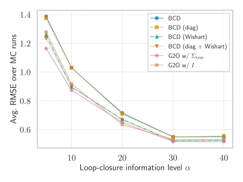
Figure 4 shows the average RMSE over Monte Carlo trials for different values of the information level $\alpha$. Figure 4(a) presents the results for the homoscedastic case, while Figures 4(b) and 4(c) show the results for the heteroscedastic case before and after additional loop closures, respectively. The results show that our framework, across all variants, succesfully produced solutions with an RMSE close to the reference setting where the true noise covariance matrix was available (g2o with $\Sigma_{\text{true}}$). For almost all values of $\alpha$ and all experiments, BCD (Wishart) and BCD (diag+Wishart) achieved a lower average RMSE compared to the other variants, highlighting the importance of incorporating a prior. Notably, this is despite the prior being assigned a small weight $w_{\text{prior}}$ and the fact that the prior estimate $\Sigma_{0}$ is not close to $\Sigma_{\text{true}}$. Incorporating a prior is particularly crucial in PGO, as we observed that the eigenvalues of $S(x)$ can become severely small in practice. In such cases, without a prior and without enforcing a minimum eigenvalue constraint $\Sigma\succeq\lambda_{\text{min}}I$, the ML estimate for the noise covariance can collapse to zero, leading to invalid results and excessive overconfidence. The average RMSE achieved by those variants with diagonal and without constraints are generally similar. Interestingly, the RMSE achieved by the diagonal variants appears to be close to that of their counterparts without this constraint, despite the true noise covariance being diagonal.

For some values of $\alpha$ in Figure 4(b), the BCD variants with the Wishart prior achieved a lower MSE than the reference solution. However, we expect that, on average, the reference solution will perform better with a larger number of Monte Carlo simulations. The RMSE trends look similar in all experiments, with the exception of a slight increase for $\alpha=30$ for BCD and BCD (diag) in Figure 4(b). In terms of RMSE, BCD variants with a Wishart prior outperform or perform comparably to the baseline with a fixed identity covariance in most cases. That said, especially under larger information levels (i.e., lower noise), this naïve baseline estimates $x$ quite accurately.

Figure 5 presents the average 2-Wasserstein distance (28) between the noise covariance matrices estimated by various BCD variants and the true covariance in both homoscedastic and heteroscedastic scenarios. In all cases, BCD variants achieved a small 2-Wasserstein error. For reference, the 2-Wasserstein error between $\mathcal{N}(0,\Sigma_{\text{true}})$ and the baseline $\mathcal{N}(0,I)$ exceeds 1, which is more than 20 times the errors attained by our algorithms. As noted in Section I, an incorrect noise covariance leads to severe overconfidence or underconfidence in the estimated state $x$ (e.g., the estimated trajectory in SLAM), potentially resulting in poor or catastrophic decisions.

The results indicate that, in most cases, diagonal BCD variants yield lower errors. This is expected, as the true noise covariance matrices are diagonal, and enforcing this prior information enhances estimation accuracy. Additionally, the MAP estimates obtained by BCD (Wishart) and BCD (diag+Wishart) outperform their ML-based counterparts. This is due to the fact that the eigenvalues of the sample covariance matrix $S(x)$ can be very small, indicating insufficient information for accurate noise covariance estimation. In such cases, the eigenvalue constraint effectively prevents a complete collapse of the estimated covariance. Interestingly, this issue was not encountered in [26] for ML estimation of the noise covariance matrix in P$n$P. This discrepancy may suggest additional challenges in estimating noise covariance in SLAM (and related) problems, which typically involve a larger number of variables and sparse, graph-structured relative measurements. In such cases, incorporating a prior estimate may be necessary for accurate identification of noise covariance matrices. Finally, Figure 5(b) illustrates that the MAP estimation error is lower for the noise covariance of loop closures compared to odometry edges. This difference is partly because the prior value based on $\Sigma_{0}$ is closer to the true noise covariance matrix for loop closures.

In this section, we present qualitative results on RIM, a large real-world 3D PGO dataset collected at Georgia Tech [8]. This dataset consists of $10,195$ poses and $29,743$ measurements. The g2o dataset includes a default noise covariance matrix, but with these default values, g2o struggles to solve the problem. Specifically, the Gauss-Newton and Dog-Leg solvers terminate after a single iteration, while the Levenberg-Marquardt solver completes 10 iterations but produces the trajectory estimate shown in Figure 6(a).

We ran BCD without and with the Wishart prior (i.e., ML and MAP estimation) for 10 outer iterations, using a single Dog-Leg iteration to optimize $x$ in each round. We set the prior parameter based on $w_{\text{prior}}=0.1$ and $\Sigma_{0}=0.01I$. The results are displayed in Figures 6(b) and 6(c), respectively. It is evident that the trajectory estimates obtained by BCD are significantly more accurate than those obtained using the original noise covariance values.

A closer visual inspection reveals that the trajectory estimated using the Wishart prior (right) appears more precise than the ML estimate (middle). This is expected, as without imposing a prior, some eigenvalues of $S(x)$ collapsed until they reached the eigenvalue constraint $\Sigma\succeq\lambda_{\text{min}}I$. In contrast, in the MAP case, the estimated covariance did not reach this lower bound.

Interestingly, despite $\Sigma_{0}$ being isotropic, the estimate obtained by BCD with the Wishart prior was not. In particular, the information matrix component associated with the $z$ coordinate was almost twice as large as those of $x$ and $y$. This likely reflects the fact that the trajectory in this dataset is relatively flat. This finding highlights that in this case, in addition to the prior, the measurements also contributed information to the estimation of the noise covariance matrix.

References

- Absil et al. [2009] P-A Absil, Robert Mahony, and Rodolphe Sepulchre. Optimization algorithms on matrix manifolds. Princeton University Press, 2009.
- Agarwal et al. [2023] Sameer Agarwal, Keir Mierle, and The Ceres Solver Team. Ceres Solver, 10 2023. URL https://github.com/ceres-solver/ceres-solver.
- Bishop and Nasrabadi [2006] Christopher M Bishop and Nasser M Nasrabadi. Pattern recognition and machine learning, volume 4. Springer, 2006.
- Boumal [2020] Nicolas Boumal. An introduction to optimization on smooth manifolds. Available online, Aug 2020. URL http://www.nicolasboumal.net/book.
- Boyd and Vandenberghe [2004] S. Boyd and L. Vandenberghe. Convex optimization. Cambridge university press, 2004.
- Cadena et al. [2016] Cesar Cadena, Luca Carlone, Henry Carrillo, Yasir Latif, Davide Scaramuzza, Jose Neira, Ian D Reid, and John J Leonard. Simultaneous localization and mapping: Present, future, and the robust-perception age. arXiv preprint arXiv:1606.05830, 2016.
- Campos et al. [2021] Carlos Campos, Richard Elvira, Juan J. Gómez, José M. M. Montiel, and Juan D. Tardós. ORB-SLAM3: An accurate open-source library for visual, visual-inertial and multi-map SLAM. IEEE Transactions on Robotics, 37(6):1874–1890, 2021.
- Carlone et al. [2015] Luca Carlone, Roberto Tron, Kostas Daniilidis, and Frank Dellaert. Initialization techniques for 3d slam: A survey on rotation estimation and its use in pose graph optimization. In 2015 IEEE international conference on robotics and automation (ICRA), pages 4597–4604. IEEE, 2015.
- Chen et al. [2023] Zhaozhong Chen, Harel Biggie, Nisar Ahmed, Simon Julier, and Christoffer Heckman. Kalman filter auto-tuning through enforcing chi-squared normalized error distributions with bayesian optimization. arXiv preprint arXiv:2306.07225, 2023.
- Dellaert and Contributors [2022] Frank Dellaert and GTSAM Contributors. borglab/gtsam, May 2022. URL https://github.com/borglab/gtsam).
- Dellaert et al. [2017] Frank Dellaert, Michael Kaess, et al. Factor graphs for robot perception. Foundations and Trends® in Robotics, 6(1-2):1–139, 2017.
- Ebadi et al. [2023] Kamak Ebadi, Lukas Bernreiter, Harel Biggie, Gavin Catt, Yun Chang, Arghya Chatterjee, Christopher E Denniston, Simon-Pierre Deschênes, Kyle Harlow, Shehryar Khattak, et al. Present and future of SLAM in extreme environments: The DARPA SubT challenge. IEEE Transactions on Robotics, 2023.
- Fontan et al. [2024a] Alejandro Fontan, Javier Civera, Tobias Fischer, and Michael Milford. Look ma, no ground truth! ground-truth-free tuning of structure from motion and visual SLAM. arXiv preprint arXiv:2412.01116, 2024a.
- Fontan et al. [2024b] Alejandro Fontan, Javier Civera, and Michael Milford. Anyfeature-vslam: Automating the usage of any chosen feature into visual SLAM. In Robotics: Science and Systems, volume 2, 2024b.
- Forsling et al. [2024] Robin Forsling, Simon J Julier, and Gustaf Hendeby. Matrix-valued measures and wishart statistics for target tracking applications. arXiv preprint arXiv:2406.00861, 2024.
- Khosoussi et al. [2019] Kasra Khosoussi, Matthew Giamou, Gaurav S Sukhatme, Shoudong Huang, Gamini Dissanayake, and Jonathan P How. Reliable graphs for SLAM. The International Journal of Robotics Research, 38(2-3):260–298, 2019.
- Kuemmerle et al. [2011] Rainer Kuemmerle, Giorgio Grisetti, Hauke Strasdat, Kurt Konolige, and Wolfram Burgard. g2o: A general framework for graph optimization. In Proc. of the IEEE Int. Conf. on Robotics and Automation (ICRA), 2011.
- Malinvaud [1980] Edmond Malinvaud. Statistical methods of econometrics. 1980.
- Olson et al. [2006] E. Olson, J. Leonard, and S. Teller. Fast iterative alignment of pose graphs with poor initial estimates. In Robotics and Automation, 2006. ICRA 2006. Proceedings 2006 IEEE International Conference on, pages 2262–2269. Ieee, 2006.
- Peng and Vidal [2023] Liangzu Peng and René Vidal. Block coordinate descent on smooth manifolds: Convergence theory and twenty-one examples. arXiv preprint arXiv:2305.14744, 2023.
- Powell [1970] MJD Powell. A new algorithm for unconstrained optimization. UKAEA, 1970.
- Seber and Wild [1989] George A. F. Seber and C. J. Wild. Nonlinear Regression. Wiley-Interscience, 1989.
- Shan et al. [2020] Tixiao Shan, Brendan Englot, Drew Meyers, Wei Wang, Carlo Ratti, and Rus Daniela. Lio-sam: Tightly-coupled lidar inertial odometry via smoothing and mapping. In IEEE/RSJ International Conference on Intelligent Robots and Systems (IROS), pages 5135–5142. IEEE, 2020.
- Triggs et al. [1999] Bill Triggs, Philip F McLauchlan, Richard I Hartley, and Andrew W Fitzgibbon. Bundle adjustment—a modern synthesis. In International workshop on vision algorithms, pages 298–372. Springer, 1999.
- Virtanen et al. [2020] Pauli Virtanen, Ralf Gommers, Travis E. Oliphant, Matt Haberland, Tyler Reddy, David Cournapeau, Evgeni Burovski, Pearu Peterson, Warren Weckesser, Jonathan Bright, Stéfan J. van der Walt, and et al. SciPy 1.0: Fundamental Algorithms for Scientific Computing in Python. Nature Methods, 17:261–272, 2020. doi: 10.1038/s41592-019-0686-2.
- Zhan et al. [2025] Tian Zhan, Chunfeng Xu, Cheng Zhang, and Ke Zhu. Generalized maximum likelihood estimation for perspective-n-point problem. IEEE Robotics and Automation Letters, 2025.
- Zhang et al. [2020] Lingyi Zhang, David Sidoti, Adam Bienkowski, Krishna R Pattipati, Yaakov Bar-Shalom, and David L Kleinman. On the identification of noise covariances and adaptive kalman filtering: A new look at a 50 year-old problem. IEEE Access, 8:59362–59388, 2020.
Appendix A Wishart Prior
Consider as a prior for the information matrix. Here we assume where is the dimension of covariance matrix and . The mode of this distribution is given by