This paper was converted on www.awesomepapers.org from LaTeX by an anonymous user.
Want to know more? Visit the Converter page.

Joint Stabilization and Regret Minimization through Switching in Over-Actuated Systems (extended version)

Jafar Abbaszadeh Chekan    Kamyar Azizzadenesheli    Cédric Langbort Coordinated Science Lab, University of Illinois at Urbana-Champaign, IL 61820 USA (e-mail: langbort & [email protected]). Department of Computer Science, Purdue University, IN 47907 USA (e-mail: [email protected])
Abstract

Adaptively controlling and minimizing regret in unknown dynamical systems while controlling the growth of the system state is crucial in real-world applications. In this work, we study the problem of stabilization and regret minimization of linear over-actuated dynamical systems. We propose an optimism-based algorithm that leverages possibility of switching between actuating modes in order to alleviate state explosion during initial time steps. We theoretically study the rate at which our algorithm learns a stabilizing controller and prove that it achieves a regret upper bound of 𝒪(T)\mathcal{O}(\sqrt{T}).

keywords:
Adaptive Control, Regret Bound, Model-Based Reinforcement Learning, Over-Actuated Systems, Online-Learning.
thanks:

1 Introduction

The past few years have witnessed a growing interest in an online learning-based Linear Quadratic (LQ) control, in which an unknown LTI system is controlled while guaranteeing a suitable scaling of the regret (defined as the average difference between the closed-loop quadratic cost and the best achievable one, with the benefit of knowing the plant’s parameters) over a desired horizon [0,T][0,T].

Table 1 summarizes the regret’s scaling achieved by several recent works in the literature (Abbasi and Szepesvári (2011); Mania et al. (2019); Cohen et al. (2019); Lale et al. (2020a)). As can be seen, the bounds scale like T\sqrt{T}, but also include an exponential term in mm (the dimension of the plant’s state plus inputs) when an initial stabilizing controller is unavailable. Recently, Chen and Hazan (2021) have shown that this dependency is unavoidable in this setting, at least for an initial exploration time period, by providing a matching lower bound. On closer inspection, this undesirable dependency stems from an exponential growth of the system’s state during the initial period of learning, which eventually contributes a 𝒪(mm)\mathcal{O}(m^{m}) term like that appearing on the last row of Table 1. Apart from negatively impacting regret, this transient state growth can also be damageable if, e.g., the linear plant to be controlled is in fact the linearization of a nonlinear process around some particular equilibrium, and the state can be driven outside the neighborhood of this equilibrium where the linearization is adequate.

A natural idea to try and partially alleviate this effect in over-actuated systems is to reduce the ambient dimension ``m"``m" during the initial period by employing only a subset of all available actuators, before potentially switching to a different mode to simultaneously learn and control the plant. The goal of this paper is to show that this approach yields the desired result (a lower bound on the plant’s state and the regret than in the presence of all actuators) and to provide a rigorous proof of the achieved 𝒪((n+di)(n+di))\mathcal{O}((n+d_{i})^{(n+d_{i})}) bound (where did_{i} is number of actuators during initial exploration). We note that, while the idea is conceptually simple, obtaining these rigorous guarantees is not completely straightforward, and requires a revisit of the tools of Lale et al. (2020a) to overcome a potential challenge: ensuring that, at the end of the period when a strict subset of actuators is used, all entries of the B-matrix (including those corresponding to unused actuators) are sufficiently well-learned for the closed-loop to become stable and the regret to remain appropriately bounded. This can only be achieved by adding additional exploratory noise with respect to the approach of Lale et al. (2020a) and results in an additional linear term in the regret bound.

Table 1: Overview of Prior Works
Algorithm Regret *
Abbasi and Szepesvári (2011) 𝒪(mmT)\mathcal{O}(m^{m}\sqrt{T}) No
Mania et al. (2019) 𝒪(poly(m)T)\mathcal{O}(poly(m)\sqrt{T}) Yes
Cohen et al. (2019) 𝒪(poly(m)T)\mathcal{O}(poly(m)\sqrt{T}) Yes
Lale et al. (2020a) 𝒪(mm)+𝒪(poly(m)T)\mathcal{O}(m^{m})+\mathcal{O}(poly(m)\sqrt{T}) No

* requirement for initial stabilizing controller.

While this idea of leveraging over-actuation can generally be applied to any model-based type of online learning algorithms presenting the exponential scaling mentioned above, we focus on the special kind of methods based on “Optimism in the Face of Uncertainty (OFU)”.

OFU type of algorithms, which couple estimation and control design procedures, have shown their ability to outperform the naive certainty equivalence algorithm. Campi and Kumar (1998) propose an OFU based approach to address the optimal control problem for LQ setting with guaranteed asymptotic optimality. However, this algorithm only guarantees the convergence of average cost to that of the optimal control in the limit but does not provide any bound on the measure of performance loss in finite time. Abbasi and Szepesvári (2011) propose a learning-based algorithm to address the adaptive control design of LQ control system in finite time with worse case regret bound of 𝒪(T)\mathcal{O}(\sqrt{T}) with exponential dependence in dimension. Using l2l_{2}-regularized least square estimation, they construct a high-probability confidence set around unknown parameters of the system and designed an algorithm that optimistically plays with respect to this set. Along this line, many works attempt to get rid of the exponential dependence with further assumption, e.g. highly sparse dynamics (see Ibrahimi et al. (2012)) or access to a stabilizing controller (see Cohen et al. (2019)). Furthermore, Faradonbeh et al. (2020) propose an OFU-based learning algorithm with mild assumptions and 𝒪(T)\mathcal{O}(\sqrt{T}) regret. This class of algorithms was extended by Lale et al. (2020b, 2021) to LQG setting where there is only partial and noisy observations on the state of system. In addition, Lale et al. (2020a) propose an algorithm with more exploration for both controllable and stabilizable systems.

The remainder of the paper is organized as follows: Section 2 reviews the preliminaries, assumptions and presents the problem statement and formulation. Section 3 overviews the proposed initial exploration (IExp), stabilizing OFU (SOFUA) algorithms and discusses in detail how to choose best actuating mode for the initial exploration purpose. Furthermore, in Section 3 the performance analysis (state norm upper-bound and regret bound) is given while leaving the details of the analysis to Section 6 and technical theorems and proofs of analysis to Section 7. Numerical experiments are given in Section 4. Finally, Section 5 summarizes the paper’s key contributions.

2 Assumptions and Problem Formulation

Consider the following linear time invariant dynamics and the associated cost functional given by:

xt+1\displaystyle x_{t+1} =Axt+But+ωt+1\displaystyle=A_{*}x_{t}+B_{*}u_{t}+\omega_{t+1} (1a)
ct\displaystyle c_{t} =xtQxt+utRut\displaystyle=x_{t}^{\top}Q_{*}x_{t}+u_{t}^{\top}R_{*}u_{t} (1b)

where the plant and input matrices An×nA_{*}\in\mathbb{R}^{n\times n} and Bn×dB_{*}\in\mathbb{R}^{n\times d} are initially unknown and have to be learned and (A,B)(A_{*},B_{*}) is controllable. Qn×nQ_{*}\in\mathbb{R}^{n\times n} and Rd×dR_{*}\in\mathbb{R}^{d\times d} represent known and positive definite matrices. ωt+1\omega_{t+1} denotes process noise, satisfying the following assumption.

Assumption 1

There exists a filtration t\mathcal{F}_{t} such that

(1.1)(1.1) 𝔼[ωt+1ωt+1|t]=σ¯ω2In\mathbb{E}[\omega_{t+1}\omega_{t+1}^{\top}|\;\mathcal{F}_{t}]=\bar{\sigma}_{\omega}^{2}I_{n} for some σ¯ω2>0\bar{\sigma}_{\omega}^{2}>0;

(1.2)(1.2) ωt\omega_{t} are component-wise sub-Gaussian, i.e., there exists σω>0\sigma_{\omega}>0 such that for any γ\gamma\in\mathbb{R} and j=1,2,,nj=1,2,...,n

𝔼[eγωj(t+1)|t]eγ2σω2/2.\displaystyle\mathbb{E}[e^{\gamma\omega_{j}(t+1)}|\;\mathcal{F}_{t}]\leq e^{\gamma^{2}\sigma_{\omega}^{2}/2}.

The problem is designing a sequence {ut}\{u_{t}\} of control inputs such that the regret T\mathcal{R}_{T} defined by

T=t=1T(xtQxt+utRutJ(Θ,Q,R))\displaystyle\mathcal{R}_{T}=\sum_{t=1}^{T}\bigg{(}x_{t}^{\top}Q_{*}x_{t}+u^{\top}_{t}R_{*}u_{t}-J_{*}(\Theta_{*},Q_{*},R_{*})\bigg{)} (2)

achieves a desired specification which scales sublinearly in TT. The term J(Θ,Q,R)J_{*}(\Theta_{*},Q_{*},R_{*}) in (2) where Θ=(AB)\Theta_{*}=(A_{*}\;B_{*})^{\top} denotes optimal average expected cost. For LQR setting with controllable pair (A,B)(A,\;B) we have J(Θ,Q,R)=σ¯ω2trace(P(Θ,Q,R))J_{*}(\Theta,Q,R)=\bar{\sigma}_{\omega}^{2}trace(P(\Theta,Q,R)), where P(Θ,Q,R)P(\Theta,Q,R) is the unique solution of discrete algebraic riccati equation (DARE) and the average expected cost minimizing policy has feedback gain of

K(Θ,Q,R)=(BP(Θ,Q,R)B+R)1BP(Θ,Q,R)A.\displaystyle K(\Theta,Q,R)=-(B^{\top}P(\Theta,Q,R)B+R)^{-1}B^{\top}P(\Theta,Q,R)A.

While the regret’s exponential dependency on system dimension appears in the long-run in Abbasi and Szepesvári (2011) the recent results of Mania et al. (2019) on the existence of a stabilizing neighborhood, makes it possible to design an algorithm that only exhibits this dependency during an initial exploration phase (see Lale et al. (2020a)).

After this period, the controller designed for any estimated value of the parameters is guaranteed to be stabilizing and the exponentially dependent term thus only appears as a constant in overall regret bound. As explained in the introduction, this suggests using only a subset of actuators during initial exploration to even further reduce the guaranteed upperbound on the state.

In the remainder of the paper, we pick the best actuating mode (i.e. subset of actuators) so as to minimize the state norm upper-bound achieved during initial exploration and characterize the needed duration of this phase for all system parameter estimates to reside in the stabilizing neighborhood. This is necessary to guarantee both closed loop stability and acceptable regret, and makes it possible to switch to the full actuation mode.

Let 𝔹\mathbb{B} be the set of all columns, bib^{i}_{*} (i{1,,d}i\in\{1,...,d\}) of BB_{*}. An element of its power set 2𝔹2^{\mathbb{B}} is a subset j\mathcal{B}_{j} j{1,,2d}j\in\{1,...,2^{d}\} of columns corresponding to a submatrix BjB_{*}^{j} of BB_{*} and mode jj. For simplicity, we assume that B1=BB^{1}_{*}=B_{*} i.e., that the first mode contains all actuators. Given this definition we write down different actuating modes dynamics with extra exploratory noise as follows

xt+1=Θizt+Bνt+ωt+1,zt=(xtuti).\displaystyle x_{t+1}={\Theta^{i}_{*}}^{\top}z_{t}+B_{*}\nu_{t}+\omega_{t+1},\quad z_{t}=\begin{pmatrix}x_{t}\\ u^{i}_{t}\end{pmatrix}. (3)

where Θi=(A,Bi)\Theta^{i}_{*}=(A_{*},B^{i}_{*})^{\top} is controllable.

The associated cost with this mode is

cti\displaystyle c^{i}_{t} =xtQxt+utiRiuti\displaystyle=x_{t}^{\top}Q_{*}x_{t}+{u^{i}_{t}}^{\top}R^{i}_{*}u^{i}_{t} (4)

where Ridi×diR_{*}^{i}\in\mathbb{R}^{d_{i}\times d_{i}} is a block of RR_{*} which penalizes the control inputs of the actuators of mode ii.

We have the following assumption on the modes which assists us in designing proposed strategy.

Assumption 2

(Side Information)

  1. 1.

    There exists sis^{i} and Υi\Upsilon_{i} such that Θi𝒮ci\Theta_{*}^{i}\in\mathcal{S}^{i}_{c} for all modes ii where

    𝒮ci=\displaystyle\mathcal{S}^{i}_{c}= {ΘiR(n+di)×ntrace(ΘiΘi)(si)2,\displaystyle\{{\Theta^{i}}\in R^{(n+d_{i})\times n}\mid trace({\Theta^{i}}^{\top}\Theta^{i})\leq({s^{i}})^{2},
    (A,Bi)(A,B^{i}) is controllable,
    A+BiK(Θi,Q,Ri)Υi<1\displaystyle\|A+B^{i}K(\Theta^{i},Q_{*},R^{i}_{*})\|\leq\Upsilon_{i}<1
    and (A,M) is observable,where Q=MM}.\displaystyle\text{and $(A,M)$ is observable,}\text{where $Q=M^{\top}M$}\}.

    .

  2. 2.

    There are known positive constants ηi\eta^{i}, ϑi\vartheta_{i}, γi\gamma^{i} such that Biϑi\|B_{*}^{i}\|\leq\vartheta_{i},

    supΘi𝒮iA+BiK(Θi,Q,Ri)ηi\displaystyle\sup_{\Theta^{i}\in\mathcal{S}^{i}}\|A_{*}+B^{i}_{*}K({\Theta}^{i},Q_{*},R^{i}_{*})\|\leq\eta^{i} (5)

    and

    J(Θi,Q,Ri)J(Θ,Q,R)γi.\displaystyle J_{*}(\Theta_{*}^{i},Q_{*},R^{i}_{*})-J_{*}(\Theta_{*},Q_{*},R_{*})\leq\gamma^{i}. (6)

    for every mode ii.

By slightly abusing notation, we drop the superscript label for the actuating mode 1 (e.g. Υ1=Υ\Upsilon_{1}=\Upsilon, s1=ss^{1}=s, and 𝒮c1=𝒮c\mathcal{S}_{c}^{1}=\mathcal{S}_{c}). It is obvious that siss^{i}\leq s i\forall i.

Note that the item (1) in Assumption 2 is typical in the literature of OFU-based algorithms (see e.g., Abbasi and Szepesvári (2011); Lale et al. (2020a)) while (2) in fact always holds in the sense that supΘi𝒮iA+BiK(Θi,Q,Ri)\sup_{\Theta^{i}\in\mathcal{S}^{i}}\|A_{*}+B^{i}_{*}K({\Theta}^{i},Q_{*},R^{i}_{*})\| and J(Θi,Q,Ri)J(Θ,Q,R)J_{*}(\Theta_{*}^{i},Q_{*},R^{i}_{*})-J_{*}(\Theta_{*},Q_{*},R_{*}) are always bounded (see e.g., Abbasi and Szepesvári (2011); Lale et al. (2020a)). The point of (2), then, is that upper-bounds on their suprema are available which can in turn be used to bound regret explicitly. The knowledge of these bounds does not affect Algorithms 1 and 2 but their value enters Algorithm 3 for determination of the best actuating mode and the corresponding exploration duration. In that sense ”best actuating mode” should be understood as ”best given the available information”.

Boundedness of SciS^{i}_{c}’s implies boundedness of P(Θi,Q,Ri)P(\Theta^{i},Q_{*},R_{*}^{i}) with a finite constant DciD_{c}^{i} (see Anderson and Moore (1971)), (i.e., Dci=sup{P(Θi,Q,Ri)Θi𝒮ci}D_{c}^{i}=\sup\{\left\lVert P(\Theta^{i},Q_{*},R_{*}^{i})\right\rVert\mid\Theta^{i}\in\mathcal{S}^{i}_{c}\}). We define D=maxiDiD=\max_{i\in\mathcal{B}^{*}}D^{i}. Furthermore, there exists κci>1\kappa^{i}_{c}>1 such that κci=sup{K(Θi,Q,Ri)Θi𝒮ci}\kappa^{i}_{c}=\sup\{\left\lVert K(\Theta^{i},Q_{*},R_{*}^{i})\right\rVert\mid\Theta^{i}\in\mathcal{S}^{i}_{c}\}.

Recalling that the set of actuators of mode ii is i\mathcal{B}_{i}, we denote its complement by ic\mathcal{B}_{i}^{c} (i.e. iic={1,,d}\mathcal{B}_{i}\cup\mathcal{B}_{i}^{c}=\{1,...,d\}). Furthermore, we denote the complement of control matrix BiB_{*}^{i} by B¯i\bar{B}^{i}_{*}.

If some modes fail to satisfy Assumption 2 they can simply be removed from the set 2𝔹2^{\mathbb{B}} without affecting algorithm or the derived guarantees.

3 Overview of Proposed Strategy

In this section, we propose an algorithm in the spirit of that first proposed by Lale et al. (2020a) which leverages actuator redundancy in the ”more exploration” step to avoid blow up in the state norm while minimizing the regret bound. We break down the strategy into two phases of initial exploration, presented by Algorithm (IExp), and optimism (Opt), given by SOFUA algorithm.

The IExp algorithm, which leverages exploratory noise, is deployed in the actuating mode ii^{*} for duration TciT_{c}^{i^{*}} to reach a stabilizing neighborhood of the full-actuation mode and alleviate state explosion while minimizing regret.

Afterwards, Algorithm 2 which leverages all the actuators comes into play. This algorithm has the central confidence set, given by the Algorithm 1, as an input. The best actuating mode ii^{*} that guarantees minimum possible state norm upper-bound and initial exploration duration TciT^{i^{*}}_{c} is determined by running Algorithm 3 at the subsection 3.3.

Algorithm 1 Initial Exploration (IExp)
1:  Inputs:TciT^{i^{*}}_{c}si>0,\,s^{i^{*}}>0,δ>0,\,\delta>0,σω,σν,λ>0\,\sigma_{\omega},\,\sigma_{\nu}\,,\lambda>0
2:  set V0i=λIV^{i^{*}}_{0}=\lambda I, Θ^i=0\hat{\Theta}^{i^{*}}=0
3:  Θ~0i=argminΘ𝒞0i(δ)SiJ(Θi,Q,Ri)\tilde{\Theta}^{i}_{0}=\arg\min_{\Theta\in\mathcal{C}^{i^{*}}_{0}(\delta)\cap S^{i}}\,\,J(\Theta^{i},Q_{*},R_{*}^{i})
4:  for t=0,1,,Tcit=0,1,...,T^{i^{*}}_{c} do
5:     if det(Vti)>2det(Vτi)\det(V^{i^{*}}_{t})>2\det(V^{i^{*}}_{\tau}) or t=0t=0 then
6:        Calculate Θ^ti\hat{\Theta}^{i^{*}}_{t} by (9) and set τ=t\tau=t
7:        Find Θ~ti\tilde{\Theta}^{i^{*}}_{t} by (11) for i=ii=i^{*}
8:     else
9:        Θ~ti=Θ~t1i\tilde{\Theta}^{i^{*}}_{t}=\tilde{\Theta}^{i^{*}}_{t-1}
10:     end if
11:     For the parameter Θ~ti\tilde{\Theta}^{i^{*}}_{t} solve the Ricatti equation and find uti=K(Θ~ti,Q,Ri)xtu^{i^{*}}_{t}=K(\tilde{\Theta}^{i^{*}}_{t},Q_{*},R_{*}^{i^{*}})x_{t}
12:     Construct u¯ti\bar{u}^{i^{*}}_{t} using (13) and apply it on the system Θ\Theta_{*} (12) and observe new state xt+1x_{t+1}.
13:     Using utiu^{i^{*}}_{t} and xtx_{t} form ziz^{i^{*}} and Save (zti,xt+1)(z^{i^{*}}_{t},x_{t+1}) into dataset
14:     Set Vt+1i=Vti+ztiztiV^{i^{*}}_{t+1}=V^{i^{*}}_{t}+z^{i^{*}}_{t}{z^{i^{*}}_{t}}^{\top} and form 𝒞t+1i\mathcal{C}^{i^{*}}_{t+1}
15:     using u¯ti\bar{u}^{i}_{t} and xtx_{t} form z¯ti\bar{z}^{i}_{t}
16:     Form (z¯ti,xt+1)(\bar{z}^{i}_{t},x_{t+1})
17:     Set Vt+1=Vt+z¯tiz¯tiV_{t+1}=V_{t}+\bar{z}^{i}_{t}{\bar{z}_{t}^{i}}^{\top} and form 𝒞t+1\mathcal{C}_{t+1}
18:  end for
19:  Return VTc+1V_{T_{c}+1} and corresponding 𝒞Tc\mathcal{C}_{T_{c}}
Algorithm 2 Stabilizing OFU Algorithm (SOFUA)
1:  Inputs:T,T,S>0,\,S>0,δ>0,\,\delta>0,Q,L,VTc,𝒞Tc,Θ^Tc\,Q\,,L,\,V_{T_{c}},\,\mathcal{C}_{T_{c}},\,\hat{\Theta}_{T_{c}}
2:  Θ~Tc=argminΘ𝒞Tc(δ)SJ(Θ)\tilde{\Theta}_{T_{c}}=argmin_{\Theta\in\mathcal{C}_{T_{c}}(\delta)\cap S}\,\,J(\Theta)
3:  for t=Tc,Tc+1,Tc+2,t=T_{c},T_{c}+1,T_{c}+2,... do
4:     if det(Vt)>2det(Vτ)\det(V_{t})>2\det(V_{\tau}) or t=Tct=T_{c} then
5:        Calculate Θ^t\hat{\Theta}_{t} by (9) and set τ=t\tau=t
6:        Find Θ~t\tilde{\Theta}_{t} by (11) for i=1i=1
7:     else
8:        Θ~t=Θ~t1\tilde{\Theta}_{t}=\tilde{\Theta}_{t-1}
9:     end if
10:     For the parameter Θ~t\tilde{\Theta}_{t} solve Ricatti and calculate u¯t=K(Θ~t,Q,R)xt\bar{u}_{t}=K(\tilde{\Theta}_{t},Q_{*},R_{*})x_{t}
11:     Apply the control on Θ\Theta_{*} and observe new state xt+1x_{t+1}.
12:     Save (zt,xt+1)(z_{t},x_{t+1}) into dataset
13:     Vt+1=Vt+ztztV_{t+1}=V_{t}+z_{t}z_{t}^{\top}
14:  end for

3.1 Main steps of Algorithm 1

3.1.1 Confidence Set Contruction

In IExp phase we add an extra exploratory Gaussian noise ν\nu to the input of all actuators even those not in actuators set of mode ii. Assuming that the system actuates in an arbitrary mode ii, the dynamics of system, used for confidence set construction (i.e. system identification), is written as

xt+1=Θiz¯ti+B¯iν¯ti+ωt+1,z¯ti=(xtu¯ti).\displaystyle x_{t+1}={\Theta^{i}_{*}}^{\top}\underline{z}^{i}_{t}+\bar{B}^{i}_{*}\bar{\nu}^{i}_{t}+\omega_{t+1},\quad\underline{z}^{i}_{t}=\begin{pmatrix}x_{t}\\ \underline{u}^{i}_{t}\end{pmatrix}. (7)

in which B¯iddi\bar{B}^{i}_{*}\in\mathbb{R}^{d-d_{i}} and u¯ti=uti+νt(i)\underline{u}^{i}_{t}=u^{i}_{t}+\nu_{t}(\mathcal{B}_{i}), and ν¯ti=νt(ic)\bar{\nu}^{i}_{t}=\nu_{t}(\mathcal{B}_{i}^{c}) where, if νtd\nu_{t}\in\mathbb{R}^{d} and 𝒩𝔹\mathcal{N}\subset\mathbb{B}, the vector ν(𝒩)card(𝒩)\nu(\mathcal{N})\in\mathbb{R}^{card(\mathcal{N})} is constructed by only keeping the entries of νt\nu_{t} corresponding to the index set of elements in 𝒩\mathcal{N}. Note that (7) is equivalent to (3) but separates used and unused actuators.

By applying self-normalized process, the least square estimation error, e(Θi)e(\Theta^{i}) can be obtained as:

e(Θi)=λTr(ΘiΘi)\displaystyle e(\Theta^{i})=\lambda\operatorname{Tr}({\Theta^{i}}^{\top}\Theta^{i})
+s=0t1Tr((xs+1Θiz¯si)(xs+1Θiz¯si)))\displaystyle+\sum_{s=0}^{t-1}\operatorname{Tr}\big{(}(x_{s+1}-{\Theta^{i}}^{\top}\underline{z}^{i}_{s})(x_{s+1}-{\Theta^{i}}^{\top}\underline{z}^{i}_{s})^{\top})\big{)} (8)

with regularization parameter λ\lambda. This yields the l2l^{2}-regularized least square estimate:

Θ^ti\displaystyle\hat{\Theta}^{i}_{t} =argminΘie(Θi)=(Z¯tiZ¯ti+λI)1Z¯tiXt\displaystyle=\operatorname*{argmin_{\Theta^{i}}}e(\Theta^{i})=({\underline{Z}_{t}^{i}}^{\top}\underline{Z}_{t}^{i}+\lambda I)^{-1}{\underline{Z}_{t}^{i}}^{\top}X_{t} (9)

where Z¯ti\underline{Z}_{t}^{i} and XtX_{t} are matrices whose rows are z¯0i,,z¯t1i{\underline{z}^{i}_{0}}^{\top},...,{\underline{z}^{i}_{t-1}}^{\top} and x1,,xtx_{1}^{\top},...,x_{t}^{\top}, respectively. Defining covariance matrix VtiV^{i^{*}}_{t} as follows:

Vti=λI+s=0t1z¯siz¯si=λI+Z¯tiZ¯ti,\displaystyle V^{i}_{t}=\lambda I+\sum_{s=0}^{t-1}\underline{z}^{i}_{s}{\underline{z}^{i}_{s}}^{\top}=\lambda I+{\underline{Z}_{t}^{i}}^{\top}\underline{Z}_{t}^{i},

it can be shown that with probability at least (1δ)(1-\delta), where 0<δ<10<\delta<1, the true parameters of system Θi\Theta^{i}_{*} belongs to the confidence set defined by (see 17):

𝒞ti(δ)\displaystyle\mathcal{C}^{i}_{t}(\delta) ={ΘiRn×(n+di)\displaystyle=\{{\Theta^{i}}^{\top}\in R^{n\times(n+d_{i})}\mid
Tr((Θ^tiΘi)Vti(Θ^tiΘi))βti(δ)},\displaystyle\operatorname{Tr}((\hat{\Theta}^{i}_{t}-\Theta^{i})^{\top}V_{t}^{i}(\hat{\Theta}^{i}_{t}-\Theta^{i}))\leq\beta^{i}_{t}(\delta)\},
βti(δ)\displaystyle\beta^{i}_{t}(\delta) =(λ1/2si+σω2nlog(ndet(Vti)1/2det(λI)1/2δ)\displaystyle=\bigg{(}\lambda^{1/2}s^{i}+\sigma_{\omega}\sqrt{2n\log(n\frac{\det(V^{i}_{t})^{1/2}\det(\lambda I)^{-1/2}}{\delta}})
+B¯iσν2dilog(didet(Vti)1/2det(λI)1/2δ))2\displaystyle+\|\bar{B}_{*}^{i}\|\sigma_{\nu}\sqrt{2d_{i}\log(d_{i}\frac{\det(V^{i}_{t})^{1/2}\det(\lambda I)^{-1/2}}{\delta}})\bigg{)}^{2} (10)

After finding high-probability confidence sets for the unknown parameter, the core step is implementing Optimism in the Face of Uncertainty (OFU) principle. At any time tt, we choose a parameter Θ~ti𝒮ci𝒞ti(δ)\tilde{\Theta}^{i}_{t}\in\mathcal{S}^{i}_{c}\cap\mathcal{C}^{i}_{t}(\delta) such that:

J(Θ~ti,Q,Ri)infΘi𝒞ti(δ)𝒮ciJ(Θi,Q,Ri)+1t.\displaystyle J(\tilde{\Theta}^{i}_{t},Q_{*},R_{*}^{i})\leq\inf\limits_{\Theta^{i}\in\mathcal{C}^{i}_{t}(\delta)\cap\mathcal{S}^{i}_{c}}J(\Theta^{i},Q_{*},R^{i}_{*})+\frac{1}{\sqrt{t}}. (11)

Then, by using the chosen parameters as if they were the true parameters, the linear feedback gain K(Θ~i,Q,Ri)K(\tilde{\Theta}^{i},Q_{*},R_{*}^{i}) is designed. We synthesized the control u¯ti=uti+νt(i)\underline{u}^{i}_{t}=u^{i}_{t}+\nu_{t}(\mathcal{B}_{i}) on (7) where uti=K(Θ~i,Q,Ri)xtu^{i}_{t}=K(\tilde{\Theta}^{i},Q_{*},R_{*}^{i})x_{t}. The extra exploratory noise νt𝒩(μ,σν2I)d\nu_{t}\sim\mathcal{N}(\mu,\,\sigma_{\nu}^{2}I)\in\mathbb{R}^{d} with σν2=2κ2σ¯ω2\sigma_{\nu}^{2}=2\kappa^{2}\bar{\sigma}_{\omega}^{2} is the random “more exploration” term.

As can be seen in the regret bound analysis, recurrent switches in policy may worsen the performance, so a criterion is needed to prevent frequent policy switches. As such, at each time step tt the algorithm checks the condition det(Vti)>2det(Vτi)\det(V^{i}_{t})>2\det(V^{i}_{\tau}) to determine whether updates to the control policy are needed where τ\tau is the last time of policy update.

3.1.2 Central Ellipsoid Construction

Note that (10) holds regardless of the control signal z¯ti\underline{z}^{i}_{t}. The formulation above also holds for any actuation mode, being mindful that the dimension of the covariance matrix changes. Even while actuating in the IExp phase, by applying augmentation technique, we can build a confidence set (which we call the central ellipsoid) around the parameters of the full actuation mode thanks to extra exploratory noise. For tTcit\leq T^{i}_{c}, this simply can be carried out by rewriting (7) as follows:

xt+1=Θz¯ti+ωt+1,z¯ti=(xtu¯ti)\displaystyle x_{t+1}=\Theta_{*}^{\top}\bar{z}^{i}_{t}+\omega_{t+1},\quad\bar{z}^{i}_{t}=\begin{pmatrix}x_{t}\\ \bar{u}^{i}_{t}\end{pmatrix} (12)

where z¯tin+d\bar{z}^{i}_{t}\in\mathbb{R}^{n+d} and u¯tid\bar{u}^{i}_{t}\in\mathbb{R}^{d} is constructed by augmentation as follows

u¯ti(i)=uti+ν(i),u¯ti(ic)=ν(ic).\displaystyle\bar{u}^{i}_{t}(\mathcal{B}_{i})=u^{i}_{t}+\nu(\mathcal{B}_{i}),\quad\bar{u}^{i}_{t}(\mathcal{B}^{c}_{i})=\nu(\mathcal{B}^{c}_{i}). (13)

By this augmentation, we can construct the central ellipsoid

𝒞t(δ)={ΘRn×(n+d)Tr((Θ^tΘ)Vt(Θ^tΘ))\displaystyle\mathcal{C}_{t}(\delta)=\{\Theta^{\top}\in R^{n\times(n+d)}\mid\operatorname{Tr}((\hat{\Theta}_{t}-\Theta)^{\top}V_{t}(\hat{\Theta}_{t}-\Theta))
βt(δ)}\displaystyle\leq\beta_{t}(\delta)\}
βt(δ)=(σω2nlog(det(Vt)1/2det(λI)1/2δ)+λ1/2s)2.\displaystyle\beta_{t}(\delta)=(\sigma_{\omega}\sqrt{2n\log(\frac{\det(V_{t})^{1/2}\det(\lambda I)^{-1/2}}{\delta}})+\lambda^{1/2}s)^{2}. (14)

which is an input to Algorithm 2 and used to compute IExp duration.

3.2 Main steps of Algorithm 2

The main steps of Algorithm 2 are quite similar to those of Algorithm 1 with a minor difference in confidence set construction. Algorithm 2 receives VTciV_{T^{i^{*}}_{c}}, ZTciZ_{T^{i^{*}}_{c}}, and XTciX_{T^{i^{*}}_{c}} from Algorithm 1, using which for t>Tcit>T^{i^{*}}_{c} we have

Vt\displaystyle V_{t} =VTci+s=Tci+1t1zszs\displaystyle=V_{T^{i^{*}}_{c}}+\sum_{s=T^{i^{*}}_{c}+1}^{t-1}{z}_{s}{{z}_{s}}^{\top}
ZtXt\displaystyle Z_{t}X_{t} =ZTciXTci+s=Tci+1t1zsxs\displaystyle=Z_{T^{i^{*}}_{c}}X_{T^{i^{*}}_{c}}^{\top}+\sum_{s=T^{i^{*}}_{c}+1}^{t-1}{z}_{s}{{x}_{s}}^{\top}

and the confidence set is easily constructed.

The following theorem summarizes boundedness of state norm when Algorithm 1 and 2 are deployed.

Theorem 3
  1. 1.

    The IExp algorithm keeps the states of the underlying system actuating in any mode ii bounded with the probability at least 1δ1-\delta during initial exploration, i.e.,

    xt\displaystyle\|x_{t}\| 11Υi(ηiΥi)n+di[GiZtn+din+di+1βti(δ)12(n+di+1)+\displaystyle\leq\frac{1}{1-\Upsilon_{i}}\big{(}\frac{\eta_{i}}{\Upsilon_{i}}\big{)}^{n+d_{i}}\bigg{[}G_{i}Z_{t}^{\frac{n+d_{i}}{n+d_{i}+1}}\beta^{i}_{t}(\delta)^{\frac{1}{2(n+d_{i}+1)}}+
    (σω2nlogntδ+sIσν2dilogditδ)]=:αti,\displaystyle\quad(\sigma_{\omega}\sqrt{2n\log\frac{nt}{\delta}}+\|sI\|\sigma_{\nu}\sqrt{2d_{i}\log\frac{d_{i}t}{\delta}})\bigg{]}=:\alpha_{t}^{i}, (15)

    for all modes i{1,,2d}i\in\{1,...,2^{d}\}.

  2. 2.

    For t>Tci+(n+di)log(n+di)+logcilogχslog21Υ:=Trct>T^{i^{*}}_{c}+\frac{(n+d_{i^{*}})\log(n+d_{i^{*}})+\log c^{i^{*}}-\log\chi_{s}}{\log\frac{2}{1-\Upsilon}}:=T_{rc} we, with probability at least 1δ1-\delta, have xt2χs\|x_{t}\|\leq 2\chi_{s} where

    χs:=2σω1Υ2nlogn(TTci)δ.\displaystyle\chi_{s}:=\frac{2\sigma_{\omega}}{1-\Upsilon}\sqrt{2n\log\frac{n(T-T^{i^{*}}_{c})}{\delta}}. (16)

From parts (1) and (2) of Theorem 3 we define the following good events:

Fti={ωΩsTci,xsαti}.\displaystyle F^{i}_{t}=\{\omega\in\Omega\mid\forall s\leq T^{i}_{c},\left\lVert x_{s}\right\rVert\leq\alpha^{i}_{t}\}. (17)

and

Ftop,c={ωΩTcist,xs2Xc2}.\displaystyle F^{op,c}_{t}=\{\omega\in\Omega\mid\forall\;\;T^{i^{*}}_{c}\leq s\leq t,\left\lVert x_{s}\right\rVert^{2}\leq X_{c}^{2}\}. (18)

in which

Xc2=32nσω2(1+κ2)(1Υ)2logn(TTc)δ.\displaystyle X_{c}^{2}=\frac{32n\sigma^{2}_{\omega}(1+\kappa^{2})}{(1-\Upsilon)^{2}}\log\frac{n(T-T_{c})}{\delta}. (19)

where both the events are used for regret bound analysis and the former one specifically is used to obtain best actuating mode for initial exploration.

3.3 Determining the Optimal Mode for IExp

We still need to specify the best actuating mode ii^{*} for initial exploration along with its corresponding upperbound XtiX_{t}^{i^{*}}. Theorem 5 specifies ii^{*}. First we need the following Lemma.

Lemma 4

At the end of initial exploration, for any mode i{1,,2d}\forall i\in\{1,...,2^{d}\} the following inequality holds

Θ^TωiΘ2μciTωi\displaystyle||\hat{\Theta}_{T^{i}_{\omega}}-\Theta_{*}||_{2}\leq\frac{\mu^{i}_{c}}{\sqrt{T^{i}_{\omega}}} (20)

where μci\mu^{i}_{c} is given as follows

μci:=\displaystyle\mu^{i}_{c}:= 1σ(σωn(n+d)log(1+𝒫cλ(n+d))+2nlog1δ+\displaystyle\frac{1}{\sigma_{\star}}\bigg{(}\sigma_{\omega}\sqrt{n(n+d)\log\big{(}1+\frac{\mathcal{P}_{c}}{\lambda(n+d)}\big{)}+2n\log\frac{1}{\delta}}+
λs)\displaystyle\sqrt{\lambda}s\bigg{)} (21)

with,

𝒫c\displaystyle\mathcal{P}_{c} :=XTωii2(1+2κi2)Tωi+4Tωiσν2dilog(dTωi/δ)\displaystyle:={X_{T^{i}_{\omega}}^{i}}^{2}(1+2{\kappa^{i}}^{2})T^{i}_{\omega}+4T^{i}_{\omega}\sigma^{2}_{\nu}d_{i}\log(dT^{i}_{\omega}/\delta)

in which TωiT^{i}_{\omega} stands for initial exploration duration of actuating in mode ii. Furthermore, if we define

Tci:=4(1+κ)2μci2(1Υ)2\displaystyle T^{i}_{c}:=\frac{4(1+\kappa)^{2}\mu^{i2}_{c}}{(1-\Upsilon)^{2}} (22)

then for Tωi>TciT^{i}_{\omega}>T^{i}_{c}, Θ^TωiΘ21Υ2(1+κ)||\hat{\Theta}_{T^{i}_{\omega}}-\Theta_{*}||_{2}\leq\frac{1-\Upsilon}{2(1+\kappa)} holds with probability at least 12δ1-2\delta.

The proof is provided in Appendix 7.

Theorem 5

Suppose Assumptions 1 and 2 hold true. Then for a system actuating in the mode ii during initial exploration phase, the following results hold true

  1. 1.

    IFtimax1stxsxtI_{F^{i}_{t}}\max_{1\leq s\leq t}\|x_{s}\|\leq x_{t} where IFtiI_{F^{i}_{t}} is indicator function of set FtiF^{i}_{t} and

    xt=Yi,tn+di+1\displaystyle x_{t}=Y_{i,t}^{n+d_{i}+1} (23)
    Yi,t:=max(e,λ(n+di)(e1),L¯i+L¯i2+4K¯i2K¯i),\displaystyle Y_{i,t}:=\max\big{(}e,\lambda(n+d^{i})(e-1),\frac{-\bar{L}_{i}+\sqrt{\bar{L}_{i}^{2}+4\bar{K}_{i}}}{2\bar{K}_{i}}\big{)},

    with

    L¯i=(𝒟1i+𝒟2i)(2nσωlog1δ+σωλsi)logt+\displaystyle\bar{L}^{i}=(\mathcal{D}^{i}_{1}+\mathcal{D}^{i}_{2})\big{(}2n\sigma_{\omega}\log\frac{1}{\delta}+\sigma_{\omega}\sqrt{\lambda}s^{i}\big{)}\log t+
    𝒟3ilogt/δ+(𝒟1i+𝒟2i)nσω(n+di)×\displaystyle\mathcal{D}^{i}_{3}\sqrt{\log t/\delta}+(\mathcal{D}^{i}_{1}+\mathcal{D}^{i}_{2})n\sigma_{\omega}(n+d_{i})\times
    (log(n+di)λ+2𝒱ti2(n+di)λt+log(1+2κi2)(n+di)λt)logt\displaystyle\bigg{(}\log\frac{(n+d_{i})\lambda+2{\mathcal{V}^{i}_{t}}^{2}}{(n+d_{i})\lambda}t+\log\frac{(1+2{\kappa^{i}}^{2})}{(n+d_{i})\lambda}t\bigg{)}\log t
    K¯i=2(𝒟1i+𝒟2i)nσω(n+di)(n+di+1)logt.\displaystyle\quad\bar{K}^{i}=2(\mathcal{D}^{i}_{1}+\mathcal{D}^{i}_{2})n\sigma_{\omega}(n+d_{i})(n+d_{i}+1)\log t.

    where

    𝒟1i:=41Υi(ηiΥi)n+diG¯i(1+2κi2)n+di2(n+di+1)\displaystyle\mathcal{D}^{i}_{1}:=\frac{4}{1-\Upsilon_{i}}\big{(}\frac{\eta_{i}}{\Upsilon_{i}}\big{)}^{n+d_{i}}\bar{G}_{i}(1+2{\kappa^{i}}^{2})^{\frac{n+d_{i}}{2(n+d_{i}+1)}}
    𝒟2i:=41Υi(ηiΥi)n+diG¯i2n+di2(n+di+1)𝒱Ti,\displaystyle\mathcal{D}^{i}_{2}:=\frac{4}{1-\Upsilon_{i}}\big{(}\frac{\eta_{i}}{\Upsilon_{i}}\big{)}^{n+d_{i}}\bar{G}_{i}2^{\frac{n+d_{i}}{2(n+d_{i}+1)}}\mathcal{V}_{T}^{i},
    𝒟3i:=n21Υi(ηiΥi)n+diσω\displaystyle\mathcal{D}^{i}_{3}:=\frac{n\sqrt{2}}{1-\Upsilon_{i}}\big{(}\frac{\eta_{i}}{\Upsilon_{i}}\big{)}^{n+d_{i}}\sigma_{\omega}

    in which 𝒱ti=σν2dilogdit/δ\mathcal{V}^{i}_{t}=\sigma_{\nu}\sqrt{2d_{i}\log d_{i}t/\delta} holds with probability least 1δ/21-\delta/2.

  2. 2.

    The best actuating mode ii^{*} for initial exploration is,

    i\displaystyle i^{*} =argmini{1,,2𝔹}Yi,Tωin+di+1\displaystyle=argmin_{i\in\{1,...,2^{\mathbb{B}}\}}Y_{i,T^{i}_{\omega}}^{n+d_{i}+1}
    s.tTωiTci\displaystyle s.t\;\;\;\;T^{i}_{\omega}\geq T^{i}_{c} (24)
  3. 3.

    The upper-bound of state norm of system actuating in the mode ii^{*} during initial exploration phase can be written as follows:

    xtcci(n+di)n+di\displaystyle\|x_{t}\|\leq c_{c}^{i^{*}}(n+d_{i^{*}})^{n+d_{i^{*}}} (25)

    for some finite system parameter-dependent constant ccic_{c}^{i^{*}}.

Remark 6

While optimization problem (24) cannot be solved analytically because TciT^{i}_{c} itself depends on xTωix_{T^{i}_{\omega}}, it can be determined using Algorithm 3.

Algorithm 3 Find best actuating mode ii^{*} and its corresponding TciT_{c}^{i^{*}}
1:  Inputs:λ,κ,Si>0,\lambda,\,\kappa,\,S^{i}>0,δ>0,\,\delta>0,,σω,ϑi,ηi,Υii\,,\sigma_{\omega},\,\vartheta_{i},\,\eta_{i},\,\Upsilon_{i}\,\forall i
2:  for i{1,,2𝔹}\forall i\in\{1,...,2^{\mathbb{B}}\} do
3:     Titri=1T^{i}_{itr}=1
4:     for t=1,2,,Titrit=1,2,...,T^{i}_{itr} do
5:        compute TciT_{c}^{i} by (22)
6:        if t<Tcit<T_{c}^{i} then
7:           Titri=Titri+1T^{i}_{itr}=T^{i}_{itr}+1
8:        else
9:           Tωi=tT^{i}_{\omega}=t
10:        end if
11:     end for
12:  end for
13:  Compute xTωi=Yi,Tωin+di+1x_{T^{i}_{\omega}}=Y_{i,T^{i}_{\omega}}^{n+d_{i}+1} i{1,,2𝔹}\forall i\in\{1,...,2^{\mathbb{B}}\}
14:  Solve i=argminixTωii^{*}=\arg\min_{i\in\mathcal{B}_{*}}x_{T^{i}_{\omega}}.
15:  Outputs: ii^{*} and TωiT^{i^{*}}_{\omega}

3.4 Regret Bound

Recall (2), the regret for the proposed strategy (IExp+
SOFUA) can be defined as follows:

T=𝔼[t=1T(xtQxt+u¯ti(t)Ru¯ti(t)J(Θ,Q,R))]\displaystyle\mathcal{R}_{T}=\mathbb{E}\left[\sum_{t=1}^{T}(x_{t}^{\top}Q_{*}x_{t}+{\bar{u}^{i(t)}_{t}}^{\top}R_{*}\bar{u}_{t}^{i(t)}-J_{*}(\Theta_{*},Q_{*},R_{*}))\right] (26)

where i(t)=ii(t)=i^{*} for tTcit\leq T^{i^{*}}_{c} and i(t)=1i(t)=1 for t>Tcit>T^{i^{*}}_{c}.

An upper-bound for T\mathcal{R}_{T} is given by the following theorem which is the next core result of our analysis.

Theorem 7

(Regret Bound of IExp+SOFUA) Under Assumptions 1 and 2, with probability at least 1δ1-\delta the algorithm SOFUA together with additional exploration algorithm IExp which runs for TciT^{i^{*}}_{c} time steps achieves regret of 𝒪((n+di)(n+di)Trci)\mathcal{O}\big{(}(n+d_{i^{*}})^{(n+d_{i^{*}})}T^{i^{*}}_{rc}\big{)} for tTcit\leq T^{i^{*}}_{c} and 𝒪(poly(n+d)TTrci)\mathcal{O}\big{(}poly(n+d)\sqrt{T-T^{i^{*}}_{rc}}\big{)} for t>Tcit>T^{i^{*}}_{c} where 𝒪(.)\mathcal{O}(.) absorbs logarithmic terms.

4 Numerical Experiment

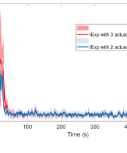
In this section, we demonstrate on a practical example how the use of our algorithms successfully alleviates state explosion during the initial exploration phase. We consider a control system with drift and control matrices to be set as follows:

A=(1.0400.270.520.810.8300.040.90),B=(0.610.290.470.580.250.500.720.29).\displaystyle A_{*}=\begin{pmatrix}1.04&0&-0.27\\ 0.52&-0.81&0.83\\ 0&0.04&-0.90\end{pmatrix},\;B_{*}=\begin{pmatrix}0.61&-0.29&-0.47\\ 0.58&0.25&-0.5\\ 0&-0.72&0.29\end{pmatrix}.

We choose the cost matrices as follows:

Q=(0.650.080.140.080.570.260.140.262.5),R=(0.140.040.050.040.240.080.050.080.2).\displaystyle Q_{*}=\begin{pmatrix}0.65&-0.08&-0.14\\ -0.08&0.57&0.26\\ -0.14&0.26&2.5\end{pmatrix},\;R_{*}=\begin{pmatrix}0.14&0.04&0.05\\ 0.04&0.24&0.08\\ 0.05&0.08&0.2\end{pmatrix}.

The Algorithm 3 outputs the exploration duration Tci=50sT^{i^{*}}_{c}=50s and best actuating mode ii^{*} for initial exploration with corresponding control matrix BiB_{*}^{i^{*}} and RiR_{*}^{i^{*}}

Bi=(0.610.290.580.2500.72),Ri=(0.140.040.040.24).\displaystyle B_{*}^{i^{*}}=\begin{pmatrix}0.61&-0.29\\ 0.58&0.25\\ 0&-0.72\end{pmatrix},\;\;\;\;\;\;R_{*}^{i^{*}}=\begin{pmatrix}0.14&0.04\\ 0.04&0.24\end{pmatrix}.
Refer to caption
Refer to caption
Figure 1: Top. State norm, Bottom. regret bound

It has graphically been shown in Abbasi-Yadkori (2013) that the optimization problem (11) is generally non-convex for n,d>1n,d>1. Because of this fact, we decided to solve optimization problem (11) using a projected gradient descent method in Algorithm 1 and 2, with basic step

Θ~t+1iPROJ𝒞ti(δ)(Θ~tiγΘi(Litr(P(Θi,Q,Ri))))\displaystyle\tilde{\Theta}^{i}_{t+1}\leftarrow PROJ_{\mathcal{C}^{i}_{t}(\delta)}\bigg{(}\tilde{\Theta}^{i}_{t}-\gamma\nabla_{\Theta^{i}}(L^{i}tr(P(\Theta^{i},Q_{*},R^{i}_{*})))\bigg{)} (27)

where Li=σ¯ω2+ϑ2σ¯ν2L^{i}=\bar{\sigma}^{2}_{\omega}+\vartheta^{2}\bar{\sigma}^{2}_{\nu} for i=ii=i^{*} and Li=σ¯ω2L^{i}=\bar{\sigma}^{2}_{\omega} for i=1i=1. Θif\nabla_{\Theta^{i}}f is the gradient of ff with respect to Θi\Theta^{i}. 𝒞ti(Θi)\mathcal{C}^{i}_{t}(\Theta^{i}) is the confidence set, PROJgPROJ_{g} is Euclidean projection on gg and finally γ\gamma is the step size. Computation of gradient Θi\nabla_{\Theta^{i}} as well as formulation of projection has been explicited in Abbasi-Yadkori (2013), similar to which we choose the learning rate as follows:

γ=0.001tr(Vti).\displaystyle\gamma=\sqrt{\frac{0.001}{tr(V^{i}_{t})}}.

We apply the gradient method for 100 iterations to solve each OFU optimization problem and apply the projection technique until the projected point lies inside the confidence ellipsoid. The inputs to the OFU algorithm are T=10000T=10000, δ=1/T\delta=1/T, λ=1\lambda=1, σω=0.1\sigma_{\omega}=0.1, s=1s=1 and we repeat simulation 1010 times.

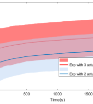
As can be seen in Fig. 1, the maximum value of the state norm (attained during the initial exploration phase) is smaller when using mode ii^{*} than when all actuators are in action.

Regret-bound for both cases is linear during initial exploration phase, however SOFUA guarantees 𝒪(T)\mathcal{O}(\sqrt{T}) regret for T>50sT>50s.

5 Conclusion

In this work, we proposed an OFU principle-based controller for over-actuated systems, which combines a step of ”more-exploration” (to produce a stabilizing neighborhood of the true parameters while guaranteeing a bounded state during exploration) with one of ”optimism”, which efficiently controls the system. Due to the redundancy, it is possible to further optimize the speed of convergence of the exploration phase to the stabilizing neighborhood by choosing over actuation modes, then to switch to full actuation to guarantee an 𝒪(T)\mathcal{O}(\sqrt{T}) regret in closed-loop, with polynomial dependency on the system dimension.

A natural extension of this work is to classes of systems in which some modes are only stabilizable. Speaking more broadly, the theme of this paper also opens the door to more applications of switching as a way to facilitate learning-based control of unknown systems, some of which are the subject of current work.

References

  • Abbasi and Szepesvári (2011) Abbasi, Y. and Szepesvári, C. (2011). Regret bounds for the adaptive control of linear quadratic systems. In Proceedings of the 24th Annual Conference on Learning Theory, 1–26.
  • Abbasi-Yadkori (2013) Abbasi-Yadkori, Y. (2013). Online learning for linearly parametrized control problems. UAlberta.
  • Anderson and Moore (1971) Anderson, B.D. and Moore, J.B. (1971). Linear Optimal Control [by] Brian DO Anderson [and] John B. Moore. Prentice-hall.
  • Bertsekas (2011) Bertsekas, D.P. (2011). Dynamic programming and optimal control 3rd edition, volume ii. Belmont, MA: Athena Scientific.
  • Campi and Kumar (1998) Campi, M.C. and Kumar, P. (1998). Adaptive linear quadratic gaussian control: the cost-biased approach revisited. SIAM Journal on Control and Optimization, 36(6), 1890–1907.
  • Chen and Hazan (2021) Chen, X. and Hazan, E. (2021). Black-box control for linear dynamical systems. In Conference on Learning Theory, 1114–1143. PMLR.
  • Cohen et al. (2019) Cohen, A., Koren, T., and Mansour, Y. (2019). Learning linear-quadratic regulators efficiently with only sqrt(t) regret. International Conference on Machine Learning, 1300–1309.
  • Faradonbeh et al. (2020) Faradonbeh, M.K.S., Tewari, A., and Michailidis, G. (2020). Optimism-based adaptive regulation of linear-quadratic systems. IEEE Transactions on Automatic Control, 66(4), 1802–1808.
  • Ibrahimi et al. (2012) Ibrahimi, M., Javanmard, A., and Roy, B.V. (2012). Efficient reinforcement learning for high dimensional linear quadratic systems. In Advances in Neural Information Processing Systems, 2636–2644.
  • Lale et al. (2020a) Lale, S., Azizzadenesheli, K., Hassibi, B., and Anandkumar, A. (2020a). Explore more and improve regret in linear quadratic regulators. arXiv preprint arXiv:2007.12291.
  • Lale et al. (2020b) Lale, S., Azizzadenesheli, K., Hassibi, B., and Anandkumar, A. (2020b). Regret bound of adaptive control in linear quadratic gaussian (lqg) systems. arXiv.
  • Lale et al. (2021) Lale, S., Azizzadenesheli, K., Hassibi, B., and Anandkumar, A. (2021). Adaptive control and regret minimization in linear quadratic gaussian (lqg) setting. In 2021 American Control Conference (ACC), 2517–2522. IEEE.
  • Mania et al. (2019) Mania, H., Tu, S., and Recht, B. (2019). Certainty equivalence is efficient for linear quadratic control. Advances in Neural Information Processing Systems, 32.

6 Analysis

In this section, we dig further and provide a numerical experiment and rigorous analysis of the algorithms, properties of the closed-loop system, and regret bounds. The most technical results, proofs and lemma can be found in the Appendix.

6.1 Stabilization via IExp (proof of Theorem 3. (1))

This section attempts to upper-bound the state norm during initial exploration phase. We carry out this part regardless of which mode has been chosen for initial exploration.

During the initial exploration the state recursion of system actuating in mode ii is written as follows:

xt+1={A~txt+B~tiuti+Bνt+Mtizti+ωttτTciAxt+Bu¯ti+ωttτTci\displaystyle x_{t+1}=\begin{cases}\tilde{A}_{t}x_{t}+\tilde{B}^{i}_{t}u_{t}^{i}+B_{*}\nu_{t}+M^{i}_{t}z^{i}_{t}+\omega_{t}&\quad t\not\in\tau_{T_{c}^{i}}\\ A_{*}x_{t}+B_{*}\bar{u}^{i}_{t}+\omega_{t}&\quad t\in\tau_{T_{c}^{i}}\\ \end{cases} (28)

where Mti=(ΘiΘ~ti)M^{i}_{t}=(\Theta^{i}_{*}-\tilde{\Theta}^{i}_{t}). The state update equation can be written as follows:

xt+1=Γtixt+rt\displaystyle x_{t+1}=\Gamma^{i}_{t}x_{t}+r_{t} (29)

where

Γt+1i={A~ti+B~tiK(Θ~ti,Q,Ri)tτTciA+BiK(Θ~ti,Q,Ri)tτTci\displaystyle\Gamma^{i}_{t+1}=\begin{cases}\tilde{A}^{i}_{t}+\tilde{B}^{i}_{t}K(\tilde{\Theta}^{i}_{t},Q_{*},R_{*}^{i})&\quad t\not\in\tau_{T_{c}^{i}}\\ A_{*}+B^{i}_{*}K(\tilde{\Theta}^{i}_{t},Q_{*},R_{*}^{i})&\quad t\in\tau_{T_{c}^{i}}\\ \end{cases} (30)

and

rt+1={Bνt+Mtizti+ωttτTciBνt+ωttτTci\displaystyle r_{t+1}=\begin{cases}B_{*}\nu_{t}+M^{i}_{t}z^{i}_{t}+\omega_{t}&\quad t\not\in\tau_{T_{c}^{i}}\\ B_{*}\nu_{t}+\omega_{t}&\quad t\in\tau_{T_{c}^{i}}\\ \end{cases} (31)

By propagating the state back to time step zero, the state update equation can be written as:

xt=s=0t1Γsix0+k=1t(s=kt1Γsi)rk.\displaystyle x_{t}=\prod_{s=0}^{t-1}\Gamma^{i}_{s}x_{0}+\sum_{k=1}^{t}\bigg{(}\prod_{s=k}^{t-1}\Gamma^{i}_{s}\bigg{)}r_{k}. (32)

Recalling Assumptions 2 we have

maxtTA+BiK(Θ~ti,Q,Ri)ηci,maxtTA~t+B~tiK(Θ~ti,Q,Ri)Υi<1.\displaystyle\max_{t\leq T}||A_{*}+B^{i}_{*}K(\tilde{\Theta}^{i}_{t},Q_{*},R_{*}^{i})||\leq\eta^{i}_{c},\;\;\;\max_{t\leq T}\|\tilde{A}_{t}+\tilde{B}_{t}^{i}K(\tilde{\Theta}^{i}_{t},Q_{*},R_{*}^{i})\|\leq\Upsilon_{i}<1. (33)

Now, by assuming x0=0x_{0}=0 it yields

xt\displaystyle\|x_{t}\| (ηiΥi)n+dik=1tΥitk+1rk(ηiΥi)n+dimax1ktrkk=1tΥitk+1\displaystyle\leq\big{(}\frac{\eta^{i}}{\Upsilon_{i}}\big{)}^{n+d_{i}}\sum_{k=1}^{t}\Upsilon_{i}^{t-k+1}\|r_{k}\|\leq\big{(}\frac{\eta^{i}}{\Upsilon_{i}}\big{)}^{n+d_{i}}\max_{1\leq k\leq t}\|r_{k}\|\sum_{k=1}^{t}\Upsilon_{i}^{t-k+1}
=11Υi(ηciΥi)n+dimax1ktrk.\displaystyle=\frac{1}{1-\Upsilon_{i}}\big{(}\frac{\eta^{i}_{c}}{\Upsilon_{i}}\big{)}^{n+d_{i}}\max_{1\leq k\leq t}\|r_{k}\|. (34)

On the other hand, we have

rk{Mkizki+Bνk+ωktτTciBνk+ωktτTci\displaystyle\|r_{k}\|\leq\begin{cases}\|M^{i}_{k}z^{i}_{k}\|+\|B_{*}\nu_{k}+\omega_{k}\|&\quad t\not\in\tau_{T_{c}^{i}}\\ \|B_{*}{\nu}_{k}+\omega_{k}\|&\quad t\in\tau_{T_{c}^{i}}\\ \end{cases} (35)

which results in

maxktrkmaxkt,tτTciMkizki+maxkt(sI)νk+ωk\displaystyle\max_{k\leq t}\|r_{k}\|\leq\max_{k\leq t,t\notin\tau_{T^{i}_{c}}}\|M^{i}_{k}z^{i}_{k}\|+\max_{k\leq t}\|(sI){\nu}_{k}+\omega_{k}\| (36)

where in second term from right hand side we applied the fact that trace(B~B~)strace(\tilde{B}^{\top}\tilde{B})\leq s (see Assumption 2).

Now applying Lemma 18 and union bound argument one can write

xt\displaystyle||x_{t}|| 11Υi(ηiΥi)n+di[GiZtn+din+di+1βti(δ)12(n+di+1)+\displaystyle\leq\frac{1}{1-\Upsilon_{i}}\big{(}\frac{\eta_{i}}{\Upsilon_{i}}\big{)}^{n+d_{i}}\bigg{[}G_{i}Z_{t}^{\frac{n+d_{i}}{n+d_{i}+1}}\beta^{i}_{t}(\delta)^{\frac{1}{2(n+d_{i}+1)}}+
(σω2nlogntδ+sIσν2dilogditδ)]=:αti,i{1,,|a|}\displaystyle\quad(\sigma_{\omega}\sqrt{2n\log\frac{nt}{\delta}}+\|sI\|\sigma_{\nu}\sqrt{2d_{i}\log\frac{d_{i}t}{\delta}})\bigg{]}=:\alpha_{t}^{i},\;\forall i\in\{1,...,|\mathcal{B}^{*}_{a}|\} (37)

where did_{i} stands for the number of actuators of an actuating mode ii and similarly any subscripts and superscripts ii denotes the actuating mode ii.

The policy explicited in Algorithm 1 keeps the states of the underlying system bounded with the probability at least 1δ1-\delta during initial exploration which is defined as the ”good event” FtiF^{i}_{t}

Fti={ωΩsTci,xsαti}.\displaystyle F^{i}_{t}=\{\omega\in\Omega\mid\forall s\leq T^{i}_{c},\left\lVert x_{s}\right\rVert\leq\alpha^{i}_{t}\}. (38)

A second ”good event” is associated with the confidence set for an arbitraty mode ii defined as:

Eti={ωΩst,Θi𝒞si(δ/4)}\displaystyle E^{i}_{t}=\{\omega\in\Omega\mid\forall s\leq t,\Theta_{*}^{i}\in\mathcal{C}^{i}_{s}(\delta/4)\} (39)

6.2 Determining the exploration time and best mode for IExp

6.2.1 Exploration duration

Given the constructed central confidence set 𝒞T\mathcal{C}_{T}, we aim to specify the time duration TciT^{i^{*}}_{c} that guarantees the parameter estimate resides within stabilizing neighborhood. For this, we need to lower bound the smallest eigenvalue of co-variance matrix VtV_{t}. The following lemma adapted from Lale et al. (2020a), named persistence of excitation during the extra exploration, provides this lower bound.

Lemma 8

For the initial exploration period of Tω6ncplog(12/δ)T_{\omega}\geq\frac{6n}{c_{p}^{\prime}}\log(12/\delta) we have

λmin(VTω)σ2Tω\displaystyle\lambda_{\min}(V_{T_{\omega}})\geq\sigma_{\star}^{2}T_{\omega} (40)

with probability at least 1δ1-\delta where σ2=cpσ1216\sigma_{\star}^{2}=\frac{c_{p}^{\prime}\sigma_{1}^{2}}{16}, cp:=min{cp,cp′′}c_{p}^{\prime}:=\min\{c_{p},c^{\prime\prime}_{p}\}, and

cp=σ¯ω2σ124σ¯ν2(1+σ222σ¯ν2)exp(σ22σ¯ν2)σ22\displaystyle c_{p}=\frac{\bar{\sigma}^{2}_{\omega}-\sigma^{2}_{1}-4\bar{\sigma}^{2}_{\nu}(1+\frac{\sigma^{2}_{2}}{2\bar{\sigma}^{2}_{\nu}})\exp(\frac{-\sigma_{2}^{2}}{\bar{\sigma}^{2}_{\nu}})}{\sigma_{2}^{2}}
cp′′=σ¯ω224σ¯ν2(1+σ322σ¯ν2)exp(σ32σ¯ν2)σ220.5σ¯ν2exp(σ322σ¯ν2)\displaystyle c^{\prime\prime}_{p}=\frac{\frac{\bar{\sigma}^{2}_{\omega}}{2}-4\bar{\sigma}^{2}_{\nu}(1+\frac{\sigma^{2}_{3}}{2\bar{\sigma}^{2}_{\nu}})\exp(\frac{-\sigma_{3}^{2}}{\bar{\sigma}^{2}_{\nu}})}{\sigma_{2}^{2}}-0.5\bar{\sigma}^{2}_{\nu}\exp(\frac{-\sigma^{2}_{3}}{2\bar{\sigma}^{2}_{\nu}})

for any σ12σ22\sigma^{2}_{1}\leq\sigma^{2}_{2} and σ32\sigma^{2}_{3} such that cp,cp′′>0c_{p},c^{\prime\prime}_{p}>0.

The following lemma gives an upper-bound for the parameter estimation error at the end of time TT which will be used to compute the minimum extra exploitation time TωT_{\omega}.

Lemma 9

Suppose assumption 1 and 2 holds. For Tpoly(σω2,σν2,nlog(1/δ)T\geq poly(\sigma_{\omega}^{2},\sigma_{\nu}^{2},n\log(1/\delta) having additional exploration leads to

Θ^TΘ21σT(σω2nlog(ndet(VT)1/2δdet(λI)1/2)+λs)\displaystyle||\hat{\Theta}_{T}-\Theta_{*}||_{2}\leq\frac{1}{\sigma_{\star}\sqrt{T}}\bigg{(}\sigma_{\omega}\sqrt{2n\log\big{(}\frac{n\det(V_{T})^{1/2}}{\delta\det(\lambda I)^{1/2}}\big{)}}+\sqrt{\lambda}s\bigg{)} (41)
{pf}

The proof is straightforward. First, a confidence set around the true but unknown parameters of the system is obtained which is given by (10). Then applying (40) given by Lemma 8 completes the proof.

There is one more step to obtain the extra exploration duration, TωT_{\omega} which is obtaining an upper-bound for the right hand side of (41). Performing such a step allows us to state the following central result.

6.2.2 Best Actuating mode for initial exploration

Given the side information Υi\Upsilon_{i} and ηi\eta_{i}s for all actuating modes i{1,,2𝔹}\forall i\in\{1,...,2^{\mathbb{B}}\}, using the bound (6.1), we aim to find an actuating mode ii^{*} that provides the lowest possible upperbound of state at first phase. This guarantees the state norm does not blow-up while minimizing the regret. The following lemma specifies the best mode ii^{*} to reach this goal. Theorem 5 gives best actuating mode for IExp and its corresponding duration.

6.3 Stabilization via SOFUA (proof of Theorem 3. (2))

After running the IExp algorithm for tTcit\leq T^{i^{*}}_{c} (or tTsit\leq T^{i^{*}}_{s}) noting that the confidence set is tight enough and we are in the stabilizing region, Algorithm 2 which leverages all the actuators comes into play. This algorithm has the central confidence set given by the Algorithm 1 as an input. The confidence ellipsoid for this phase is given as follows:

𝒞t(δ)\displaystyle\mathcal{C}_{t}(\delta) ={Θ(n+d)×n\displaystyle=\{{\Theta}\in\mathbb{R}^{(n+d)\times n}\mid
Tr((Θ^tΘ)Vt(Θ^tΘ))βt(δ)}\displaystyle\quad\operatorname{Tr}((\hat{\Theta}_{t}-\Theta)^{\top}V_{t}(\hat{\Theta}_{t}-\Theta))\leq\beta_{t}(\delta)\} (42)

where

βt(δ)=(σω2nlog(det(Vt)1/2det(λI)1/2δ)+λ1/2s)2\displaystyle\beta_{t}(\delta)=(\sigma_{\omega}\sqrt{2n\log(\frac{\det(V_{t})^{1/2}\det(\lambda I)^{-1/2}}{\delta}})+\lambda^{1/2}s)^{2} (43)

and

Vt=VTei+Tei+1tztzt.\displaystyle V_{t}=V_{T^{i^{*}}_{e}}+\sum_{T^{i^{*}}_{e}+1}^{t}z_{t}z_{t}^{\top}. (44)

Now, we can define the good event EtE_{t} for time t>Tcit>T^{i^{*}}_{c}

Et={ωΩTcist,Θ𝒞s(δ/4)}.\displaystyle E_{t}=\{\omega\in\Omega\mid\forall T^{i^{*}}_{c}\leq s\leq t,\Theta_{*}\in\mathcal{C}_{s}(\delta/4)\}. (45)

Now, we are ready to upperbound the state norm.

SOFUA keeps the states of the underlying system bounded with probability at least 1δ1-\delta. In this section, we define the ”good event” FtopF^{op}_{t} for t>Tcit>T_{c}^{i^{*}}.

Noting that for t>Tcit>T_{c}^{i^{*}} the algorithm stops applying the exploratory noise ν\nu, the state dynamics is written as follows: dynamics

xt+1=\displaystyle x_{t+1}= (A+BK(Θ~t,Q,R))xt+ωt=Mtxt+ωt\displaystyle\big{(}A_{*}+B_{*}K(\tilde{\Theta}_{t},Q_{*},R_{*})\big{)}x_{t}+\omega_{t}=M_{t}x_{t}+\omega_{t} (46)

where

Mt\displaystyle M_{t} =(AA~t1+A~t1+BK(Θ~t,Q,R)\displaystyle=\big{(}A_{*}-\tilde{A}_{t-1}+\tilde{A}_{t-1}+B_{*}K(\tilde{\Theta}_{t},Q_{*},R_{*})
+B~tK(Θ~t,Q,R)B~t1K(Θ~t,Q,R)).\displaystyle+\tilde{B}_{t}K(\tilde{\Theta}_{t},Q_{*},R_{*})-\tilde{B}_{t-1}K(\tilde{\Theta}_{t},Q_{*},R_{*})\big{)}.

With controllability assumption for the t>Tcit>T^{i^{*}}_{c}, if the event EtE_{t} holds then Mt<1+Υ2<1\|M_{t}\|<\frac{1+\Upsilon}{2}<1 for all tTcit\geq T^{i^{*}}_{c}. Then starting from state xTcix_{T^{i^{*}}_{c}} one can write

xt(1+Υ2)tTcixTci+21ΥmaxTcistωs.\displaystyle\|x_{t}\|\leq\big{(}\frac{1+\Upsilon}{2}\big{)}^{t-T^{i^{*}}_{c}}\|x_{T^{i^{*}}_{c}}\|+\frac{2}{1-\Upsilon}\max_{T^{i^{*}}_{c}\leq s\leq t}\|\omega_{s}\|. (47)

By applying union bound argument on the second term from right hand side of (47) and using the bound (25), it is straight forward to show that

xt\displaystyle\|x_{t}\| (1+Υ2)tTcici(n+di)n+di+χs\displaystyle\leq\big{(}\frac{1+\Upsilon}{2}\big{)}^{t-T^{i^{*}}_{c}}c^{i^{*}}(n+d_{i^{*}})^{n+d_{i^{*}}}+\chi_{s}

where

χs:=2σω1Υ2nlogn(TTci)δ.\displaystyle\chi_{s}:=\frac{2\sigma_{\omega}}{1-\Upsilon}\sqrt{2n\log\frac{n(T-T^{i^{*}}_{c})}{\delta}}. (48)

For t>Tci+(n+di)log(n+di)+logcilogχslog21Υ:=Trct>T^{i^{*}}_{c}+\frac{(n+d_{i^{*}})\log(n+d_{i^{*}})+\log c^{i^{*}}-\log\chi_{s}}{\log\frac{2}{1-\Upsilon}}:=T_{rc} we have xt2χs\|x_{t}\|\leq 2\chi_{s}. Now the ”good event” Ftop,cF^{op,c}_{t} is defined by

Ftop,c={ωΩTcist,xs2Xc2}.\displaystyle F^{op,c}_{t}=\{\omega\in\Omega\mid\forall\;\;T^{i^{*}}_{c}\leq s\leq t,\left\lVert x_{s}\right\rVert^{2}\leq X_{c}^{2}\}. (49)

in which

Xc2=32nσω2(1+κ2)(1Υ)2logn(TTc)δ\displaystyle X_{c}^{2}=\frac{32n\sigma^{2}_{\omega}(1+\kappa^{2})}{(1-\Upsilon)^{2}}\log\frac{n(T-T_{c})}{\delta} (50)

.

6.4 Regret Bound Analysis

6.4.1 Regret decomposition

From definition of regret, one can write

T\displaystyle\mathcal{R}_{T} =t=1T(xtQxt+u¯ti(t)Ru¯ti(t))TJ(Θ,Q,R)\displaystyle=\sum_{t=1}^{T}(x_{t}^{\top}Q_{*}x_{t}+{\bar{u}^{i(t)}_{t}}^{\top}R_{*}\bar{u}_{t}^{i(t)})-TJ_{*}(\Theta_{*},Q_{*},R_{*})
=t=0Tω(xtQxt+utiRiuti+2νtRu¯ti+νtRνt)TJ(Θ,Q,R)\displaystyle=\sum_{t=0}^{T_{\omega}}\bigg{(}x_{t}^{\top}Qx_{t}+{u^{i^{*}}_{t}}^{\top}R_{*}^{i^{*}}u^{i^{*}}_{t}+2{\nu_{t}}^{\top}R_{*}{\bar{u}^{i^{*}}_{t}}+{\nu_{t}}^{\top}R_{*}\nu_{t}\bigg{)}-TJ_{*}(\Theta_{*},Q_{*},R_{*})
+t=Tω+1T(xtQxt+u¯tRu¯t)\displaystyle+\sum_{t=T_{\omega}+1}^{T}(x_{t}^{\top}Q_{*}x_{t}+{\bar{u}_{t}}^{\top}R_{*}\bar{u}_{t}) (51)

Applying Bellman optimality equation (see Bertsekas (2011)) for LQ systems actuating in any mode i=i,1i=i^{*},1, one can write

J(Θ~t1i,Q,Ri)+xtP(Θ~t1i,Q,Ri)xt\displaystyle J(\tilde{\Theta}_{t-1}^{i},Q_{*},R_{*}^{i})+x_{t}^{\top}P(\tilde{\Theta}_{t-1}^{i},Q_{*},R_{*}^{i})x_{t}
=xtQxt+utiRiuti+𝔼[(A~t1xt+B~t1iuti+ζt)P(Θ~t1i,Q,Ri)(A~t1xt+B~t1iu¯ti+ζt)|t1]\displaystyle=x_{t}^{\top}Q_{*}x_{t}+{u^{i}_{t}}^{\top}R_{*}^{i}u^{i}_{t}+\mathbb{E}\bigg{[}\big{(}\tilde{A}_{t-1}x_{t}+\tilde{B}^{i}_{t-1}u^{i}_{t}+\zeta_{t}\big{)}^{\top}P(\tilde{\Theta}_{t-1}^{i},Q_{*},R_{*}^{i})\big{(}\tilde{A}_{t-1}x_{t}+\tilde{B}^{i}_{t-1}\underline{u}^{i}_{t}+\zeta_{t}\big{)}|\mathcal{F}_{t-1}\bigg{]}
=xtQxt+uitRiuti\displaystyle=x_{t}^{\top}Q_{*}x_{t}+{u^{i}}_{t}^{\top}R_{*}^{i}u^{i}_{t}
+𝔼[(A~t1xt+B~t1iuti)P(Θ~t1i,Q,Ri)(A~t1xt+B~t1iuti)|t1]+𝔼[ζtP(Θ~t1i,Q,Ri)ζt|t1]\displaystyle+\mathbb{E}\big{[}\big{(}\tilde{A}_{t-1}x_{t}+\tilde{B}^{i}_{t-1}u^{i}_{t}\big{)}^{\top}P(\tilde{\Theta}_{t-1}^{i},Q_{*},R_{*}^{i})\big{(}\tilde{A}_{t-1}x_{t}+\tilde{B}^{i}_{t-1}u^{i}_{t}\big{)}|\mathcal{F}_{t-1}\big{]}+\mathbb{E}\big{[}\zeta_{t}^{\top}P(\tilde{\Theta}_{t-1}^{i},Q_{*},R_{*}^{i})\zeta_{t}|\mathcal{F}_{t-1}\big{]}
=xtQxt+uitRiuti+𝔼[(A~t1xt+B~t1iuti)P(Θ~t1i,Q,Ri)(A~t1xt+B~t1iuti)|t1]\displaystyle=x_{t}^{\top}Qx_{t}+{u^{i}}_{t}^{\top}R^{i}u^{i}_{t}+\mathbb{E}\big{[}\big{(}\tilde{A}_{t-1}x_{t}+\tilde{B}^{i}_{t-1}u^{i}_{t}\big{)}^{\top}P(\tilde{\Theta}_{t-1}^{i},Q_{*},R_{*}^{i})\big{(}\tilde{A}_{t-1}x_{t}+\tilde{B}^{i}_{t-1}u^{i}_{t}\big{)}|\mathcal{F}_{t-1}\big{]}
+𝔼[xt+1P(Θ~t1i,Q,Ri)xt+1|t1]𝔼[(Axt+Biuti)P(Θ~t1i,Q,Ri)(Axt+Biuti)|t1]\displaystyle+\mathbb{E}\bigg{[}x_{t+1}^{\top}P(\tilde{\Theta}_{t-1}^{i},Q_{*},R_{*}^{i})x_{t+1}|\mathcal{F}_{t-1}\bigg{]}-\mathbb{E}\big{[}\big{(}A_{*}x_{t}+B^{i}_{*}u^{i}_{t}\big{)}^{\top}P(\tilde{\Theta}_{t-1}^{i},Q_{*},R_{*}^{i})\big{(}A_{*}x_{t}+B^{i}_{*}u^{i}_{t}\big{)}|\mathcal{F}_{t-1}\big{]}
=xtQxt+utiRiuti+𝔼[xt+1P(Θ~t1i,Q,Ri)xt+1|t1]\displaystyle=x_{t}^{\top}Qx_{t}+{u^{i}_{t}}^{\top}R^{i}u^{i}_{t}+\mathbb{E}\bigg{[}x_{t+1}^{\top}P(\tilde{\Theta}_{t-1}^{i},Q_{*},R_{*}^{i})x_{t+1}|\mathcal{F}_{t-1}\bigg{]}
+(A~t1xt+B~t1iuti)P(Θ~t1i,Q,Ri)(A~t1xt+B~t1iuti)(Axt+Biuti)P(Θ~t1i,Q,Ri)(Axt+Biuti)\displaystyle+\big{(}\tilde{A}_{t-1}x_{t}+\tilde{B}^{i}_{t-1}u^{i}_{t}\big{)}^{\top}P(\tilde{\Theta}_{t-1}^{i},Q_{*},R_{*}^{i})\big{(}\tilde{A}_{t-1}x_{t}+\tilde{B}^{i}_{t-1}u^{i}_{t}\big{)}-\big{(}A_{*}x_{t}+B^{i}_{*}u^{i}_{t}\big{)}^{\top}P(\tilde{\Theta}_{t-1}^{i},Q_{*},R_{*}^{i})\big{(}A_{*}x_{t}+B^{i}_{*}u^{i}_{t}\big{)}

where ζt=Biνt(i)+ωt\zeta_{t}=B^{i}_{*}\nu_{t}(\mathcal{B}_{i})+\omega_{t} for tTωt\leq T_{\omega} and ζt=ωt\zeta_{t}=\omega_{t} for t>Tωt>T_{\omega} and with slight abuse of notation ut1=u¯tu_{t}^{1}=\bar{u}_{t}. In third equality we applied the dynamics xt+1=Axt+Biuti+ζx_{t+1}=A_{*}x_{t}+B^{i}_{*}u_{t}^{i}+\zeta and used the martingale property of process noise ζt\zeta_{t}.

Now taking summation up to time T>TωT>T_{\omega} and redefining J(Θi,Q,R)=σζ2Tr(P(Θi,Q,R))J(\Theta^{i},Q_{*},R_{*})={\sigma_{\zeta}}^{2}Tr(P(\Theta^{i},Q_{*},R_{*})) gives

t=0T(xtQxt+uti(t)Ri(t)uti(t))=t=0TJ(Θ~t1i(t),Q,Ri(t))+R1R2R3\displaystyle\sum_{t=0}^{T}\bigg{(}x_{t}^{\top}Qx_{t}+{u^{i(t)}_{t}}^{\top}R^{i(t)}{u}^{i(t)}_{t}\bigg{)}=\sum_{t=0}^{T}J(\tilde{\Theta}^{i(t)}_{t-1},Q_{*},R^{i(t)}_{*})+R_{1}-R_{2}-R_{3} (52)
=t=0Tω(σν2Tr(P(Θ~t1i,Q,Ri))BiBi)\displaystyle=\sum_{t=0}^{T_{\omega}}\bigg{(}\sigma^{2}_{\nu}Tr(P(\tilde{\Theta}_{t-1}^{i^{*}},Q_{*},R^{i^{*}}_{*}))B^{i^{*}}_{*}{B_{*}^{i^{*}}}^{\top}\bigg{)} (53)
+t=0Tω(σ¯ω2Tr(P(Θ~t1i,Q,Ri)))+t=Tω+1T(σ¯ω2Tr(P(Θ~t1,Q,R)))+R1R2R3\displaystyle+\sum_{t=0}^{T_{\omega}}\bigg{(}\bar{\sigma}^{2}_{\omega}Tr(P(\tilde{\Theta}_{t-1}^{i^{*}},Q_{*},R^{i^{*}}_{*}))\bigg{)}+\sum_{t=T_{\omega}+1}^{T}\bigg{(}\bar{\sigma}^{2}_{\omega}Tr(P(\tilde{\Theta}_{t-1},Q_{*},R_{*}))\bigg{)}+R_{1}-R_{2}-R_{3} (54)

where

R1=t=0T(xtP(Θ~t1i(t),Q,Ri(t))xt𝔼[xt+1P(Θ~ti(t),Q,Ri(t))xt+1|t1]),\displaystyle R_{1}=\sum_{t=0}^{T}\bigg{(}x^{\top}_{t}P(\tilde{\Theta}^{i(t)}_{t-1},Q_{*},R_{*}^{i(t)})x_{t}-\mathbb{E}\big{[}x^{\top}_{t+1}P(\tilde{\Theta}^{i(t)}_{t},Q_{*},R_{*}^{i(t)})x_{t+1}|\mathcal{F}_{t-1}\big{]}\bigg{)}, (55)
R2=t=0T𝔼[xt+1(P(Θ~t1i(t),Q,Ri(t))P(Θ~ti(t),Q,Ri(t)))xt+1|t1]\displaystyle R_{2}=\sum_{t=0}^{T}\mathbb{E}[x_{t+1}^{\top}\big{(}P(\tilde{\Theta}_{t-1}^{i(t)},Q_{*},R_{*}^{i(t)})-P(\tilde{\Theta}_{t}^{i(t)},Q_{*},R_{*}^{i(t)})\big{)}x_{t+1}|\mathcal{F}_{t-1}] (56)

and

R3\displaystyle R_{3} =t=0T((A~t1xt+B~t1i(t)uti(t))Pi(Θ~t1i)(A~t1xt+B~t1iuti(t))\displaystyle=\sum_{t=0}^{T}\bigg{(}(\tilde{A}_{t-1}x_{t}+\tilde{B}^{i(t)}_{t-1}{u}^{i(t)}_{t})^{\top}P^{i}(\tilde{\Theta}^{i}_{t-1})(\tilde{A}_{t-1}x_{t}+\tilde{B}^{i}_{t-1}{u}^{i(t)}_{t})
(Axt+Bi(t)uti(t))P(Θ~t1i(t),Q,Ri(t))(Axt+Bi(t)uti(t)))\displaystyle\quad-(A_{*}x_{t}+B_{*}^{i(t)}{u}^{i(t)}_{t})^{\top}P(\tilde{\Theta}^{i(t)}_{t-1},Q_{*},R_{*}^{i(t)})(A_{*}x_{t}+B^{i(t)}_{*}{u}^{i(t)}_{t})\bigg{)} (57)

with i(t)=ii(t)=i^{*} for tTωt\leq T_{\omega}, and i(t)=1i(t)=1 when t>Tωt>T_{\omega} for which we drop the corresponding super/sub scripts abusively.

Recalling optimal average cost value formula and taking into account that the extra exploratory noise νt\nu_{t} is independent of process noise ωt\omega_{t}, for duration t<Tωt<T_{\omega} that system actuates in the mode ii^{*}, the term J(Θ~t1i,Q,Ri)J(\tilde{\Theta}^{i^{*}}_{t-1},Q_{*},R_{*}^{i^{*}}) is decomposed as follows

J(Θ~t1i,Q,Ri)=σν2Tr(P(Θ~t1i,Q,Ri)BiBi)+σ¯ω2Tr(P(Θ~t1i,Q,Ri)).\displaystyle J(\tilde{\Theta}^{i^{*}}_{t-1},Q_{*},R_{*}^{i^{*}})=\sigma_{\nu}^{2}Tr\big{(}P(\tilde{\Theta}^{i^{*}}_{t-1},Q_{*},R_{*}^{i^{*}})B^{i^{*}}_{*}{B^{i^{*}}_{*}}^{\top}\big{)}+\bar{\sigma}_{\omega}^{2}Tr\big{(}P(\tilde{\Theta}^{i^{*}}_{t-1},Q_{*},R_{*}^{i^{*}})\big{)}. (58)

From given side information (6) (Assumption 2), one can write

σ¯ω2Tr(P(Θ~t1i,Q,Ri))=J(Θ~t1i,Q,Ri)J(Θ~t1i,Q,Ri)\displaystyle\bar{\sigma}_{\omega}^{2}Tr(P(\tilde{\Theta}^{i^{*}}_{t-1},Q_{*},R_{*}^{i^{*}}))=J(\tilde{\Theta}^{i^{*}}_{t-1},Q_{*},R_{*}^{i^{*}})\leq J(\tilde{\Theta}^{i^{*}}_{t-1},Q_{*},R_{*}^{i^{*}})
J(Θ,Q,R)+γi\displaystyle\leq J(\Theta_{*},Q_{*},R_{*})+\gamma^{i^{*}} (59)

which results in

t=0T(xtQxt+uti(t)Ri(t)uti(t))σν2TωDBiF2+TJ(Θ,ωt)+Tωγi+R1R2R3\displaystyle\sum_{t=0}^{T}\bigg{(}x_{t}^{\top}Q_{*}x_{t}+{{u}_{t}^{i(t)}}^{\top}R_{*}^{i(t)}{u}^{i(t)}_{t}\bigg{)}\leq\sigma_{\nu}^{2}T_{\omega}D||B^{i^{*}}_{*}||_{F}^{2}+TJ_{*}(\Theta_{*},\omega_{t})+T_{\omega}\gamma^{i^{*}}+R_{1}-R_{2}-R_{3} (60)

Combining (59) with (54) and (51) for both controllable settings under the events FTciiETciF^{i^{*}}_{T_{c}^{i^{*}}}\cap E_{T_{c}^{i^{*}}} for tTcit\leq T_{c}^{i^{*}} and FToptETF^{opt}_{T}\cap E_{T} for tTcit\geq T_{c}^{i^{*}} (and for stabilizable setting with its corresponding events) the regret can be upper-bounded as follows:

(T)\displaystyle\mathcal{R}(T) σν2TωDBiF2+γiTω+R0+R1R2R3\displaystyle\leq\sigma_{\nu}^{2}T_{\omega}D||B^{i^{*}}_{*}||_{F}^{2}+\gamma^{i^{*}}T_{\omega}+R_{0}+R_{1}-R_{2}-R_{3} (61)

where

R0=t=0Tω(2νtRu¯ti+νtRνt).\displaystyle R_{0}=\sum_{t=0}^{T_{\omega}}\big{(}2{\nu_{t}}^{\top}R_{*}\underline{u}^{i^{*}}_{t}+{\nu_{t}}^{\top}R_{*}\nu_{t}\big{)}. (62)

The term R0R_{0} given by (62) which is direct effect of extra exploratory noise on the regret bound has same upper-bound for both controllable and stabilizable settings which is given by following lemma.

Lemma 10

(Bounding R0R_{0}) On the event EFiE\cap F^{i^{*}}, the term R0R_{0} defined by (62) has the following upper bound:

|R0|d\displaystyle|R_{0}|\leq d σνBδ+dRσν2\displaystyle\sigma_{\nu}\sqrt{B_{\delta}}+d\|R_{*}\|\sigma^{2}_{\nu}
×(Tω+Tωlog4dTωδlog4δ)\displaystyle\times\big{(}T_{\omega}+\sqrt{T_{\omega}}\log\frac{4dT_{\omega}}{\delta}\sqrt{\log\frac{4}{\delta}}\big{)} (63)

where

Bδ=8(1+Tωκ2R2(n+di)2(n+di))\displaystyle B_{\delta}=8\big{(}1+T_{\omega}\kappa^{2}\|R_{*}\|^{2}(n+d_{i^{*}})^{2(n+d_{i^{*}})}\big{)}
×log(4dδ(1+Tωκ2R2(n+di)2(n+di))1/2)\displaystyle\times\log\bigg{(}\frac{4d}{\delta}\big{(}1+T_{\omega}\kappa^{2}\|R_{*}\|^{2}(n+d_{i^{*}})^{2(n+d_{i^{*}})}\big{)}^{1/2}\bigg{)}

The following subsequent sections gives rest of upperbounds.

Lemma 11

(Bounding R1R_{1}) On the event FTciiETciiF^{i^{*}}_{T_{c}^{i^{*}}}\cap E^{i^{*}}_{T_{c}^{i^{*}}} for tTcit\leq T_{c}^{i^{*}} and FTc,opETcF^{c,op}_{T}\cap E^{c}_{T} for tTcit\geq T_{c}^{i^{*}}, with probability at least 1δ/21-\delta/2 for t>Trct>T_{rc} the term R1R_{1} is upper-bounded as follows:

R1\displaystyle R_{1} kc,1(n+di)(n+di)(σω+Bσν)\displaystyle\leq k_{c,1}(n+d_{i^{*}})^{(n+d_{i^{*}})}(\sigma_{\omega}+||B_{*}||\sigma_{\nu})
×nTcilog((n+d)Tci/δ)\displaystyle\quad\times n\sqrt{T_{c}^{i^{*}}}\log((n+d^{*})T_{c}^{i^{*}}/\delta)
+kc,2σω2nn(1Γ)tTcilog(n(tTci)/δ)\displaystyle\quad+k_{c,2}\sigma^{2}_{\omega}\frac{n\sqrt{n}}{(1-\Gamma)}\sqrt{t-T_{c}^{i^{*}}}\log\big{(}n(t-T_{c}^{i^{*}})/\delta\big{)}
+kc,3nσω2tTωlog(nt/δ)\displaystyle\quad+k_{c,3}n\sigma^{2}_{\omega}\sqrt{t-T_{\omega}}\log(nt/\delta)
+kc,4n(σω+Bσν)2Tωlog(nt/δ)\displaystyle\quad+k_{c,4}n(\sigma_{\omega}+||B_{*}||\sigma_{\nu})^{2}\sqrt{T_{\omega}}\log(nt/\delta) (64)

for some problem dependent coefficients kc,1,kc,2,kc,3,kc,4k_{c,1},k_{c,2},k_{c,3},k_{c,4}.

{pf}

Proof follows as same steps as of Lale et al. (2020a), with only difference that exploration phase is performed through actuating in the mode ii^{*} with corresponding number of actuators did_{i^{*}}.

The following lemma upper-bounds the term R2R_{2}.

Lemma 12

(Bounding |R2||R_{2}|) On the event FTciiETciiF^{i^{*}}_{T_{c}^{i^{*}}}\cap E^{i^{*}}_{T_{c}^{i^{*}}} for tTcit\leq T_{c}^{i^{*}} and FTc,opETcF^{c,op}_{T}\cap E^{c}_{T} for tTcit\geq T_{c}^{i^{*}}, it holds true that the term R2R_{2} defined by (56) is upper-bounded as

|R2|2Dci2(n+di)2(n+di)\displaystyle|R_{2}|\leq 2D{c^{i^{*}}}^{2}(n+d_{i^{*}})^{2(n+d_{i^{*}})}
×{1+log2(1+ci2(1+2κi2)(n+di)2(n+di)Tci+4σν2dilog8diTiδTiλ)n+di}\displaystyle\quad\times\big{\{}1+\log_{2}\bigg{(}1+\frac{{c^{i^{*}}}^{2}(1+2{\kappa^{i}}^{2})(n+d_{i^{*}})^{2(n+d_{i^{*}})}T^{i^{*}}_{c}+4\sigma^{2}_{\nu}d_{i^{*}}\log\frac{8d_{i^{*}}T^{i^{*}}}{\delta}T^{i^{*}}}{\lambda}\bigg{)}^{n+d_{i^{*}}}\big{\}}
+2D32nσω2(1+κ2)(1Υ)2logn(TTci)δlog2(λ¯σ2(Tci+1))n+d\displaystyle\quad+2D\frac{32n\sigma^{2}_{\omega}(1+\kappa^{2})}{(1-\Upsilon)^{2}}\log\frac{n(T-T_{c}^{i^{*}})}{\delta}\log_{2}\big{(}\frac{\bar{\lambda}}{\sigma_{\star}^{2}(T_{c}^{i^{*}}+1)}\big{)}^{n+d} (65)

in which

λ¯\displaystyle\bar{\lambda} :=λ¯:=λ+ci2Tci(n+di)2(n+di)(1+2κi2)\displaystyle:=\bar{\lambda}:=\lambda+{c^{i^{*}}}^{2}T^{i^{*}}_{c}(n+d_{i^{*}})^{2(n+d_{i^{*}})}(1+2{\kappa^{i}}^{2})
+4σν2dilog(diTci/δ)\displaystyle\quad+4\sigma^{2}_{\nu}d_{i^{*}}\log(d_{i^{*}}T^{i^{*}}_{c}/\delta)
+(TTci)32nσω2(1+κ2)(1Υ)2logn(TTci)δ.\displaystyle\quad+(T-T^{i^{*}}_{c})\frac{32n\sigma^{2}_{\omega}(1+\kappa^{2})}{(1-\Upsilon)^{2}}\log\frac{n(T-T^{i^{*}}_{c})}{\delta}.

The proof can be found in Appendix 7

Lemma 13

(Bounding |R3||R_{3}|) On the event FTciiETciiF^{i^{*}}_{T_{c}^{i^{*}}}\cap E^{i^{*}}_{T_{c}^{i^{*}}} for tTcit\leq T_{c}^{i^{*}} and FTc,opETcF^{c,op}_{T}\cap E^{c}_{T} for tTcit\geq T_{c}^{i^{*}}, the term R3R_{3} defined by (57) has the following upper bound:

|R3|=𝒪((n+di)(2(n+di))Tci+(n+d)n2TTci)\displaystyle|R_{3}|=\mathcal{O}\big{(}(n+d_{i^{*}})^{(2(n+d_{i^{*}}))}T_{c}^{i^{*}}+(n+d)n^{2}\sqrt{T-T_{c}^{i^{*}}}\big{)} (66)

Putting Everything Together, gives the overall regret bound which holds with probability at least 1δ1-\delta. This bound has been summarized by Theorem 7.

7 Appendix

7.1 Technical Theorems and Lemmas

Lemma 14

(Norm of Sub-gaussian vector) For an entry-wise RR-subgaussian vector ymy\in\mathbb{R}^{m} the following upper-bound holds with probability at least 1δ1-\delta

yR2mlog(mδ)\displaystyle\|y\|\leq R\sqrt{2m\log(\frac{m}{\delta})}
Lemma 15

(Self-normalized bound for vector-valued martingales Abbasi and Szepesvári (2011)) Let FkF_{k} be a filtration, zkz_{k} be a stochastic process adapted to FkF_{k} and ωki\omega^{i}_{k} (where ωki\omega^{i}_{k} is the ii-th element of noise vector ωk\omega_{k}) be a real-valued martingale difference, again adapted to filtration FkF_{k} which satisfies the conditionally sub-Gaussianity assumption (Assumption 2.4) with known constant σω\sigma_{\omega}. Consider the martingale and co-variance matrices:

Sti:=k=1tzk1ωki,Vt=λI+1βs=1t1ztztT\displaystyle S^{i}_{t}:=\sum_{k=1}^{t}z_{k-1}\omega^{i}_{k},\quad V_{t}=\lambda I+\frac{1}{\beta}\sum_{s=1}^{t-1}z_{t}z_{t}^{T}

then with probability of at least 1δ1-\delta, 0<δ<10<\delta<1 we have,

StiVt122σω2log(det(Vt)1/2δdet(λI)1/2)\displaystyle\left\lVert S^{i}_{t}\right\rVert^{2}_{V_{t}^{-1}}\leq 2\sigma_{\omega}^{2}\log\bigg{(}\frac{\det(V_{t})^{1/2}}{\delta\det(\lambda I)^{1/2}}\bigg{)} (67)

Given the fact that for controllable systems solving DARE gives a unique stabilizing controller, in this section we go through an important result from literature that show there is a strongly stabilizing neigborhood around the parameters of a system. This means that solving DARE for any parameter value in this neighborhood gives a controller which stabilizes the system with true parameters.

Lemma 16

(Mania et al. Mania et al. (2019)) There exists explicit constants C0C_{0} and

ϵ=poly(α¯1,α¯,A,B,σ¯ω,D,n,d)\displaystyle\epsilon=poly(\underline{\alpha}^{-1},\bar{\alpha},\|A_{*}\|,\|B_{*}\|,\bar{\sigma}_{\omega},D,n,d)

in which α¯IQα¯I\underline{\alpha}I\leq Q\leq\bar{\alpha}I and α¯IRα¯I\underline{\alpha}I\leq R\leq\bar{\alpha}I such that for any Θ{n×(n+d)|ΘΘε, 0εϵ}\Theta^{\prime}\in\{\mathbb{R}^{n\times(n+d)}\;|\;\|\Theta^{\prime}-\Theta_{*}\|\leq\varepsilon,\;0\leq\varepsilon\leq\epsilon\}, we have

J(K(Θ),Θ,Q,R)JC0ε2\displaystyle J(K(\Theta^{\prime}),\Theta_{*},Q,R)-J^{*}\leq C_{0}\varepsilon^{2} (68)

where J(K(Θ),Θ,Q,R)J(K(\Theta^{\prime}),\Theta_{*},Q,R) is infinite horizon performance of policy K(Θ)K(\Theta^{\prime}) applied on Θ\Theta_{*}.

Lemma 16 implicitly says that for any estimates residing within stabilizing neighborhood, the designed controller, applied on true system, is stabilizing.

7.2 Confidence Set Construction

The following theorem gives the confidence set for initial exploration phase and actuating mode ii. Central confidence set and confidence set of actuating mode 1 can be similarly constructed.

Theorem 17

(System Identification) Consider linear dynamics model (7) where ωt\omega_{t} and νt\nu_{t} are independent random vectors, both satisfying Assumption 1 with a known σω\sigma_{\omega} and σν\sigma_{\nu}. Let trace(ΘiΘi)strace({\Theta^{i}}^{\top}\Theta^{i})\leq s (which is part of Assumptions 2) hold and Θ^ti\hat{\Theta}^{i}_{t} be l2l_{2}- regularized least square estimation at time tt. Then with probability at least 1δ1-\delta we have Θi𝒞ti(δ)\Theta^{i}_{*}\in\mathcal{C}_{t}^{i}(\delta) where

𝒞ti(δ)\displaystyle\mathcal{C}^{i}_{t}(\delta) ={ΘiRn×(n+di)\displaystyle=\{{\Theta^{i}}^{\top}\in R^{n\times(n+d_{i})}\mid
Tr((Θ^tiΘi)Vti(Θ^tiΘi))βti(δ)},\displaystyle\operatorname{Tr}((\hat{\Theta}^{i}_{t}-\Theta^{i})^{\top}V_{t}^{i}(\hat{\Theta}^{i}_{t}-\Theta^{i}))\leq\beta^{i}_{t}(\delta)\},
βti(δ)\displaystyle\beta^{i}_{t}(\delta) =(λ1/2si+σω2nlog(ndet(Vti)1/2det(λI)1/2δ)\displaystyle=\bigg{(}\lambda^{1/2}s^{i}+\sigma_{\omega}\sqrt{2n\log(n\frac{\det(V^{i}_{t})^{1/2}\det(\lambda I)^{-1/2}}{\delta}})
+B¯iσν2dilog(didet(Vti)1/2det(λI)1/2δ))2\displaystyle+\|\bar{B}_{*}^{i}\|\sigma_{\nu}\sqrt{2d_{i}\log(d_{i}\frac{\det(V^{i}_{t})^{1/2}\det(\lambda I)^{-1/2}}{\delta}})\bigg{)}^{2} (69)
{pf}

From (9) we have:

Θ^ti\displaystyle\hat{\Theta}^{i}_{t} =argminΘie(Θi)=(Z¯tiZ¯ti+λI)1Z¯tiXt\displaystyle=\operatorname*{argmin_{\Theta^{i}}}e(\Theta^{i})=({\underline{Z}_{t}^{i}}^{\top}\underline{Z}_{t}^{i}+\lambda I)^{-1}{\underline{Z}_{t}^{i}}^{\top}X_{t} (70)

where Z¯ti\underline{Z}_{t}^{i} and XtX_{t} are matrices whose rows are z¯0i,,z¯t1i{\underline{z}^{i}_{0}}^{\top},...,{\underline{z}^{i}_{t-1}}^{\top} and x1,,xtx_{1}^{\top},...,x_{t}^{\top}, respectively. and on the other hand considering the definition of XtX_{t}, Z¯ti\underline{Z}_{t}^{i} and WtW_{t} whose rows are (B¯iν¯0i+ω0)(\bar{B}^{i}_{*}\bar{\nu}^{i}_{0}+\omega_{0})^{\top},…, (B¯iν¯t1i+ωt1)(\bar{B}^{i}_{*}\bar{\nu}^{i}_{t-1}+\omega_{t-1})^{\top} the dynamic of system can be written as

Xt=Z¯tiΘi+Wt\displaystyle X_{t}=\underline{Z}_{t}^{i}\Theta_{*}^{i}+W_{t}

which leads to

Θ^ti\displaystyle\hat{\Theta}^{i}_{t} =(Z¯tiZ¯ti+λI)1Z¯ti(Z¯tiΘi+Wt)\displaystyle=({\underline{Z}^{i}_{t}}^{\top}{\underline{Z}^{i}_{t}}+\lambda I)^{-1}{\underline{Z}^{i}_{t}}^{\top}(\underline{Z}^{i}_{t}\Theta_{*}^{i}+W_{t})
=(Z¯tiZ¯ti+λI)1(Z¯tiZ¯ti+λI)Θiλ(Z¯tiZ¯ti+λI)1Θi\displaystyle\quad=({\underline{Z}^{i}_{t}}^{\top}{\underline{Z}^{i}_{t}}+\lambda I)^{-1}({\underline{Z}^{i}_{t}}^{\top}\underline{Z}^{i}_{t}+\lambda I)\Theta^{i}_{*}-\lambda({\underline{Z}^{i}_{t}}^{\top}{\underline{Z}^{i}_{t}}+\lambda I)^{-1}\Theta^{i}_{*}
+(Z¯tiZ¯ti+λI)1Z¯tiWt\displaystyle\quad+({\underline{Z}^{i}_{t}}^{\top}{\underline{Z}^{i}_{t}}+\lambda I)^{-1}{\underline{Z}^{i}_{t}}^{\top}W_{t}

Noting definition Vti=Z¯tiZ¯ti+λIV^{i}_{t}={\underline{Z}^{i}_{t}}^{\top}{\underline{Z}}^{i}_{t}+\lambda I it yields

Θ^tiΘi\displaystyle\hat{\Theta}^{i}_{t}-\Theta^{i}_{*} =Vti1Z¯tiWt+Vti1λΘi.\displaystyle={{V}^{i}_{t}}^{-1}{\underline{Z}_{t}^{i}}^{\top}W_{t}+{V^{i}_{t}}^{-1}\lambda\Theta^{i}_{*}. (71)

For an arbitrary random covariate ziz^{i} we have,

ziΘ^tiziΘi\displaystyle{z^{i}}^{\top}\hat{\Theta}^{i}_{t}-{z^{i}}^{\top}\Theta^{i}_{*} =zi,Z¯tiWtVti1+zi,λΘiVti1.\displaystyle=\langle\,z^{i},{\underline{Z}^{i}_{t}}^{\top}W_{t}\rangle_{{V^{i}_{t}}^{-1}}+\langle\,z^{i},\lambda\Theta^{i}_{*}\rangle_{{V^{i}_{t}}^{-1}}. (72)

By taking norm on both sides one can write,

ziΘ^tiziΘi\displaystyle\|{z^{i}}^{\top}\hat{\Theta}^{i}_{t}-{z^{i}}^{\top}\Theta^{i}_{*}\| ziVti1(Z¯tWtVti1+λΘiV¯t1)ziVti1(Z¯tWtVti1+λsi).\displaystyle\leq\|z^{i}\|_{{V^{i}_{t}}^{-1}}\Bigg{(}\|{\underline{Z}}^{\top}_{t}W_{t}\|_{{V^{i}_{t}}^{-1}}+\|\lambda\Theta^{i}_{*}\|_{\bar{V}_{t}^{-1}}\Bigg{)}\leq\|z^{i}\|_{{V^{i}_{t}}^{-1}}\Bigg{(}\|{\underline{Z}}^{\top}_{t}W_{t}\|_{{V^{i}_{t}}^{-1}}+\sqrt{\lambda}s^{i}\Bigg{)}. (73)

where in last inequality we applied the Θi2si2\|\Theta^{i}_{*}\|^{2}\leq{s^{i}}^{2} (from Assumptions 2 and LABEL:Assumption3) and teh fact that Vti11/λ{V^{i}_{t}}^{-1}\leq 1/\lambda.

Using Lemma 15, Z¯tiWtVti1\|{\underline{Z}^{i}_{t}}^{\top}W_{t}\|_{{V^{i}_{t}}^{-1}} is bounded from above as

Z¯tiWtVti1\displaystyle\|{\underline{Z}^{i}_{t}}^{\top}W_{t}\|_{{V^{i}_{t}}^{-1}} σω2nlog(ndet(Vti)1/2det(λI)1/2δ)+B¯iσν2dilog(didet(Vti)1/2det(λI)1/2δ).\displaystyle\leq\sigma_{\omega}\sqrt{2n\log(\frac{n\det(V^{i}_{t})^{1/2}\det(\lambda I)^{-1/2}}{\delta}})+\|\bar{B}_{*}^{i}\|\sigma_{\nu}\sqrt{2d_{i}\log(\frac{d_{i}\det(V^{i}_{t})^{1/2}\det(\lambda I)^{-1/2}}{\delta}}). (74)

By arbitrarily choosing zi=Vti(Θ^tiΘi)z^{i}=V^{i}_{t}(\hat{\Theta}_{t}^{i}-\Theta^{i}_{*}) and plugging it into (73) it yields

Θ^tiΘiVti2Vti(Θ^tiΘi)Vti1\displaystyle\|\hat{\Theta}^{i}_{t}-\Theta^{i}_{*}\ \|^{2}_{V^{i}_{t}}\leq\|{V}^{i}_{t}(\hat{\Theta}_{t}^{i}-\Theta^{i}_{*})\|_{{V^{i}_{t}}^{-1}}
(σω2nlog(det(Vti)1/2det(λI(n+di)×(n+di))1/2δ)+B¯iσν2dilog(didet(Vti)1/2det(λI(n+di)×(n+di))1/2δ)+λsi)\displaystyle\quad\Bigg{(}\sigma_{\omega}\sqrt{2n\log(\frac{\det({V}^{i}_{t})^{1/2}\det(\lambda I_{(n+d_{i})\times(n+d_{i})})^{-1/2}}{\delta}})+\|\bar{B}_{*}^{i}\|\sigma_{\nu}\sqrt{2d_{i}\log(\frac{d_{i}\det({V}^{i}_{t})^{1/2}\det(\lambda I_{(n+d_{i})\times(n+d_{i})})^{-1/2}}{\delta}})+\sqrt{\lambda}s^{i}\Bigg{)}

and since Θ^tiΘiVti=Vti(Θ^tiΘi)Vti1\|\hat{\Theta}^{i}_{t}-\Theta^{i}_{*}\|_{V^{i}_{t}}=\|{V}^{i}_{t}(\hat{\Theta}^{i}_{t}-\Theta^{i}_{*})\|_{{V^{i}_{t}}^{-1}}, the statement of Theorem 17 holds true.

Lemma 18

(Abbasi and Szepesvári (2011)) For any 0tT0\leq t\leq T and {1,,2𝔹}\forall\in\{1,...,2^{\mathbb{B}}\} we have that

maxst,sτt(ΘiΘ^si)zsiGZn+din+di+1βti(δ/4)12(n+di+1)\displaystyle\max_{s\leq t,s\notin\tau_{t}}||(\Theta^{i}_{*}-\hat{\Theta}^{i}_{s})^{\top}z^{i}_{s}||\leq GZ^{\frac{n+d_{i}}{n+d_{i}+1}}\beta^{i}_{t}(\delta/4)^{\frac{1}{2(n+d_{i}+1)}} (75)

where τt\tau_{t} is a set of finite number of times, with maximum cardinality n+din+d_{i}, occurring between any time interval [0t][0\;t] such that (ΘiΘ^si)zsi||(\Theta^{i}_{*}-\hat{\Theta}^{i}_{s})^{\top}z^{i}_{s}|| is not well controlled in those instances (see Lemma 17 and 18 of Abbasi and Szepesvári (2011) for more details).

During initial exploration, while the system actuate in an arbitrary mode ii it constructs the central ellipsoid by using augmentation technique. The following lemma gives an upper-bound for the determinant of co-variance matrix of mode ii, ViV^{i} and that of central ellipsoid VV (for central ellipsoid i=1i=1).

Lemma 19

Let the system actuate in an arbitrary mode ii and applies extra exploratory noise ν\nu. Further assume that the central ellipsoid is constructed by applying augmentation technique. Then with probability at least 1δ1-\delta the determinant of the co-variance matrix ViV^{i} (i=1i=1 denotes the central ellipsoid) is given by

det(Vti)det(λI(n+di)×(n+di))\displaystyle\frac{\det(V^{i}_{t})}{\det(\lambda I_{(n+d_{i})\times(n+d_{i})})}\leq
((n+di)λ+(1+2κi2)xt2t+2𝒱ti2t(n+di)λ)n+di\displaystyle\Bigg{(}\frac{(n+d_{i})\lambda+(1+2{\kappa^{i}}^{2}){x_{t}}^{2}t+2{\mathcal{V}^{i}_{t}}^{2}t}{(n+d_{i})\lambda}\Bigg{)}^{n+d_{i}} (76)

where 𝒱ti=σν2dilogdit/δ\mathcal{V}^{i}_{t}=\sigma_{\nu}\sqrt{2d_{i}\log d_{i}t/\delta}.

{pf}

we can write

det(Vti)\displaystyle det(V^{i}_{t}) j=1n+di(λ+k=1t1zjik2)\displaystyle\leq\prod_{j=1}^{n+d_{i}}\Big{(}\lambda+\sum_{k=1}^{t-1}{z^{i}_{j}}_{k}^{2}\Big{)}
(j=1n+di(λ+k=1t1zjik2)n+d)n+di\displaystyle\quad\leq\bigg{(}\frac{\sum_{j=1}^{n+d_{i}}\big{(}\lambda+\sum_{k=1}^{t-1}{z^{i}_{j}}_{k}^{2}\big{)}}{n+d}\bigg{)}^{n+d_{i}}
((n+di)λ+k=1t1xk2+2uki+2ν(i)k2n+di)n+di\displaystyle\quad\leq\Bigg{(}\frac{(n+d_{i})\lambda+\sum_{k=1}^{t-1}\|x_{k}\|^{2}+2\|u^{i}_{k}\|+2\|\nu(\mathcal{B}_{i})_{k}\|^{2}}{n+d_{i}}\Bigg{)}^{n+d_{i}}

In second inequality, we applied AM-GM inequality and in the third inequality we apply the property (a+b)22a2+2b2(a+b)^{2}\leq 2a^{2}+2b^{2}. Furthermore, uki2κi2xk2\|u^{i}_{k}\|^{2}\leq{\kappa^{i}}^{2}\|x_{k}\|^{2}. Given max0ktνk=𝒱ti\max_{0\leq k\leq t}||\nu_{k}||=\mathcal{V}^{i}_{t} one can write:

det(Vti)det(λI(n+di)×(n+di))\displaystyle\frac{\det(V^{i}_{t})}{\det(\lambda I_{(n+d_{i})\times(n+d_{i})})}\leq
((n+di)λ+(1+2κi2)xt2t+2𝒱ti2t(n+di)λ)n+di\displaystyle\Bigg{(}\frac{(n+d_{i})\lambda+(1+2{\kappa^{i}}^{2}){x_{t}}^{2}t+2{\mathcal{V}^{i}_{t}}^{2}t}{(n+d_{i})\lambda}\Bigg{)}^{n+d_{i}} (77)

where 𝒱ti=σν2dilogdit/δ\mathcal{V}^{i}_{t}=\sigma_{\nu}\sqrt{2d_{i}\log d_{i}t/\delta} holds with probability least 1δ/21-\delta/2. This completes the proof of (20). Proof of the second statement of lemma is given in Lale et al. (2020a).

7.3 Proofs of Lemma 4 and Theorem 5

{pf}

(Proof of Lemma 4). The proof directly follows by plaguing the upper-bound of det(Vt)det(V_{t}) into Lemma 9.

det(Vt)\displaystyle det(V_{t}) i=1n+d(λ+k=1t1zki2)\displaystyle\leq\prod_{i=1}^{n+d}\Big{(}\lambda+\sum_{k=1}^{t-1}z_{ki}^{2}\Big{)}
(i=1n+d(λ+k=1t1zki2)n+d)n+d\displaystyle\quad\leq\bigg{(}\frac{\sum_{i=1}^{n+d}\big{(}\lambda+\sum_{k=1}^{t-1}z_{ki}^{2}\big{)}}{n+d}\bigg{)}^{n+d}
=((n+d)λ+k=1t1z¯ki2+2ζk2n+d)n+d\displaystyle\quad=\Bigg{(}\frac{(n+d)\lambda+\sum_{k=1}^{t-1}||\bar{z}^{i^{*}}_{k}||^{2}+2||\zeta_{k}||^{2}}{n+d}\Bigg{)}^{n+d}

In second inequality we applied AM-GM inequality and in the third inequality we apply the property (a+b)22a2+2b2(a+b)^{2}\leq 2a^{2}+2b^{2}. Furthermore, z¯ki2(1+2κ2)Xe2||\bar{z}^{i^{*}}_{k}||^{2}\leq(1+2\kappa^{2})X_{e}^{2}. Given ζt2σνdlog(4nt(t+1)/δ)||\zeta_{t}||\leq 2\sigma_{\nu}\sqrt{d\log(4nt(t+1)/\delta)} which holds with probability at least 1δ/21-\delta/2 one can write:

det(Vt)det(λI(n+d)×(n+d))\displaystyle\frac{\det(V_{t})}{\det(\lambda I_{(n+d)\times(n+d)})}\leq
((n+d)λ+ci(n+d)2(n+d)(1+2κ2)t+4σν2(dd)log(8nt(t+1)/δ)(n+d)λ)n+d\displaystyle\Bigg{(}\frac{(n+d)\lambda+c^{i^{*}}(n+d^{*})^{2(n+d^{*})}(1+2\kappa^{2})t+4\sigma^{2}_{\nu}(d-d^{*})\log(8nt(t+1)/\delta)}{(n+d)\lambda}\Bigg{)}^{n+d} (78)

This completes the proof of (20). Proof of the second statement of lemma is given in Lale et al. (2020a).

{pf}

(Proof of Theorem 5) Given (6.1), we first upper-bound the term GiZTn+din+di+1βti(δ/4)12(n+di+1)G_{i}Z_{T}^{\frac{n+d_{i}}{n+d_{i}+1}}\beta^{i}_{t}(\delta/4)^{\frac{1}{2(n+d_{i}+1)}}. First, we can write

ZTi2=max0tTzt2max0tTxt2+max0tTuti+νt(i)2max0tTxt2+2uti2+2max0tTνt(i)2\displaystyle{Z^{i}_{T}}^{2}=\max_{0\leq t\leq T}\|z_{t}\|^{2}\leq\max_{0\leq t\leq T}\|x_{t}\|^{2}+\max_{0\leq t\leq T}\|u^{i}_{t}+\nu_{t}(\mathcal{B}_{i})\|^{2}\leq\max_{0\leq t\leq T}\|x_{t}\|^{2}+2\|u^{i}_{t}\|^{2}+2\max_{0\leq t\leq T}\|\nu_{t}(\mathcal{B}_{i})\|^{2}\leq
(1+2κi2)max0tTxt2+2max0tTνt(i)2\displaystyle(1+2{\kappa^{i}}^{2})\max_{0\leq t\leq T}\|x_{t}\|^{2}+2\max_{0\leq t\leq T}\|\nu_{t}(\mathcal{B}_{i})\|^{2} (79)

which results in

ZTi=max0tTzti(1+2κi2)xT+2𝒱Ti\displaystyle{Z^{i}_{T}}=\max_{0\leq t\leq T}||z^{i}_{t}||\leq\sqrt{(1+2{\kappa^{i}}^{2})}x_{T}+\sqrt{2}\mathcal{V}_{T}^{i} (80)

where xT:=max0tTxtx_{T}:=\max_{0\leq t\leq T}||x_{t}|| and 𝒱Ti:=max0tTνt(i)\mathcal{V}_{T}^{i}:=\max_{0\leq t\leq T}||\nu_{t}(\mathcal{B}_{i})||. On the other hand, given the definition of βti(δ/4)\beta^{i}_{t}(\delta/4) one can write:

βti(δ/4)12(n+di+1)βti(δ/4)124βti(δ)\displaystyle\beta^{i}_{t}(\delta/4)^{\frac{1}{2(n+d_{i}+1)}}\leq\beta^{i}_{t}(\delta/4)^{\frac{1}{2}}\leq 4\sqrt{\beta^{i}_{t}(\delta)} (81)

Combining the results give:

GiZTin+din+di+1βti(δ/4)12(n+di+1)\displaystyle G_{i}{Z^{i}_{T}}^{\frac{n+d_{i}}{n+d_{i}+1}}\beta^{i}_{t}(\delta/4)^{\frac{1}{2(n+d_{i}+1)}} 4Giβti(δ)(1+2κi2xT+2𝒱Ti)n+din+di+1\displaystyle\leq 4G_{i}\sqrt{\beta^{i}_{t}(\delta)}\big{(}\sqrt{1+2{\kappa^{i}}^{2}}x_{T}+\sqrt{2}\mathcal{V}_{T}^{i}\big{)}^{\frac{n+d_{i}}{n+d_{i}+1}} (82)
4Giβti(δ)((1+2κi2)n+di2(n+di+1)xTn+din+di+1+2n+di2(n+di+1)𝒱Tin+din+di+1)\displaystyle 4G_{i}\sqrt{\beta^{i}_{t}(\delta)}\big{(}(1+2{\kappa^{i}}^{2})^{\frac{n+d_{i}}{2(n+d_{i}+1)}}{x_{T}}^{\frac{n+d_{i}}{n+d_{i}+1}}+2^{\frac{n+d_{i}}{2(n+d_{i}+1)}}{\mathcal{V}_{T}^{i}}^{\frac{n+d_{i}}{n+d_{i}+1}}\big{)} (83)

We also have

Gi=2(2S(n+di)n+di+12U0.5)1/(n+di+1)\displaystyle G_{i}=2\bigg{(}\frac{2S(n+d_{i})^{\frac{n+d_{i}+1}{2}}}{U^{0.5}}\bigg{)}^{1/(n+d_{i}+1)}

where

Ui=U0HandU0i=116n+di2(1S2(n+di2))\displaystyle U^{i}=\frac{U_{0}}{H}\;\;\;\;and\;\;\;U^{i}_{0}=\frac{1}{16^{n+d_{i}-2}(1\vee S^{2(n+d_{i}-2)})}

One can simply rewrite GiG_{i} as follows:

Gi=𝒞H12(n+di+1)\displaystyle G_{i}=\mathcal{C}H^{\frac{1}{2(n+d_{i}+1)}}

where

𝒞:=2(2S(n+di)(16n+di2(1S2(n+di2)))1/2)1/(n+di+1)\displaystyle\mathcal{C}:=2\bigg{(}2S(n+d_{i})\big{(}16^{n+d_{i}-2}(1\vee S^{2(n+d_{i}-2)})\big{)}^{1/2}\bigg{)}^{1/(n+d_{i}+1)}

and

Hi>(164S2Mi2(n+di)U0i)\displaystyle H_{i}>\bigg{(}16\vee\frac{4S^{2}M_{i}^{2}}{(n+d_{i})U^{i}_{0}}\bigg{)}

with MiM_{i} to be defined as follows

Mi=supY>0B¯iσνn(n+di)log(1+TY/λ(n+di)δ)+σωn(n+di)log(1+TY/λ(n+di)δ)+λ1/2siY\displaystyle M_{i}=\sup_{Y>0}\frac{\|\bar{B}_{*}^{i}\|\sigma_{\nu}\sqrt{n(n+d_{i})\log\big{(}\frac{1+TY/\lambda(n+d_{i})}{\delta}\big{)}}+\sigma_{\omega}\sqrt{n(n+d_{i})\log\big{(}\frac{1+TY/\lambda(n+d_{i})}{\delta}\big{)}}+\lambda^{1/2}s^{i}}{Y}

Given the fact that Y=sup0tTztY=\sup_{0\leq t\leq T}||z_{t}||. Then by having nonzero initial state x0x_{0} then by defining Y=(1+2κi2)x0+2𝒱TiY^{*}=\sqrt{(1+2{\kappa^{i}}^{2})}\|x_{0}\|+\sqrt{2}\mathcal{V}_{T}^{i} we have the following upper-bound for MM

MiB¯iσνn(n+di)log(1+TY/λ(n+di)δ)+σωn(n+di)log(1+TY/λ(n+di)δ)+λ1/2siY:=Mmaxi.\displaystyle M_{i}\leq\frac{\|\bar{B}_{*}^{i}\|\sigma_{\nu}\sqrt{n(n+d_{i})\log\big{(}\frac{1+TY^{*}/\lambda(n+d_{i})}{\delta}\big{)}}+\sigma_{\omega}\sqrt{n(n+d_{i})\log\big{(}\frac{1+TY^{*}/\lambda(n+d_{i})}{\delta}\big{)}}+\lambda^{1/2}s^{i}}{Y^{*}}:=M_{max}^{i}.

Then we can upper bound GiG_{i} as follows

Gi𝒞(164S2Mmaxi2(n+di)U0i):=G¯i\displaystyle G_{i}\leq\mathcal{C}\bigg{(}16\vee\frac{4S^{2}M_{max}^{i2}}{(n+d_{i})U^{i}_{0}}\bigg{)}:=\bar{G}_{i}

Hence, the state norm is bounded as follows:

xt𝒟1iβti(δ)log(t)Xn+din+di+1+𝒟2ilogtδ.\displaystyle||x_{t}||\leq\mathcal{D}^{i}_{1}\sqrt{\beta^{i}_{t}(\delta)}\log(t)X^{\frac{n+d_{i}}{n+d_{i}+1}}+\mathcal{D}^{i}_{2}\sqrt{\log\frac{t}{\delta}}.

Adopted from Abbasi and Szepesvári (2011), it yields

Xt(𝒟1iβti(δ)log(t)+𝒟2iβti(δ)log(t)+𝒟3ilogtδ)n+di\displaystyle X_{t}\leq\big{(}\mathcal{D}^{i}_{1}\sqrt{\beta^{i}_{t}(\delta)}\log(t)+\mathcal{D}^{i}_{2}\sqrt{\beta^{i}_{t}(\delta)}\log(t)+\mathcal{D}^{i}_{3}\sqrt{\log\frac{t}{\delta}}\big{)}^{n+d_{i}}

where

𝒟1i:=41Υi(ηiΥi)n+diG¯i(1+2κi2)n+di2(n+di+1)\displaystyle\mathcal{D}^{i}_{1}:=\frac{4}{1-\Upsilon_{i}}\big{(}\frac{\eta_{i}}{\Upsilon_{i}}\big{)}^{n+d_{i}}\bar{G}_{i}(1+2{\kappa^{i}}^{2})^{\frac{n+d_{i}}{2(n+d_{i}+1)}}
𝒟2i:=41Υi(ηiΥi)n+diG¯i2n+di2(n+di+1)𝒱Ti\displaystyle\mathcal{D}^{i}_{2}:=\frac{4}{1-\Upsilon_{i}}\big{(}\frac{\eta_{i}}{\Upsilon_{i}}\big{)}^{n+d_{i}}\bar{G}_{i}2^{\frac{n+d_{i}}{2(n+d_{i}+1)}}\mathcal{V}_{T}^{i}
𝒟3i:=n21Υi(ηiΥi)n+diσω\displaystyle\mathcal{D}^{i}_{3}:=\frac{n\sqrt{2}}{1-\Upsilon_{i}}\big{(}\frac{\eta_{i}}{\Upsilon_{i}}\big{)}^{n+d_{i}}\sigma_{\omega}

By elementary but tedious calculations one can show

βti(δ)2nσωlog1δ+σωλsi+nσωlogdet(Vti)det(λI(n+di)×(n+di))\displaystyle\sqrt{\beta_{t}^{i}(\delta)}\leq 2n\sigma_{\omega}\log\frac{1}{\delta}+\sigma_{\omega}\sqrt{\lambda}s^{i}+n\sigma_{\omega}\log\frac{\det(V^{i}_{t})}{\det(\lambda I_{(n+d_{i})\times(n+d_{i})})}

An upper bound for the third term in the right hand side is given by applying Lemma 4. Letting at=Xt1//(n+di+1)a_{t}=X_{t}^{1//(n+d_{i}+1)} and c=max{1,max1stas}c=\max\{1,\max_{1\leq s\leq t}||a_{s}||\} results in

nσωlogdet(Vti)det(λI(n+di)×(n+di))nσω(n+di)(log(n+di)λ+2𝒱ti2(n+di)λt+log(1+2κi2)c2(n+di)λt)\displaystyle n\sigma_{\omega}\log\frac{\det(V^{i}_{t})}{\det(\lambda I_{(n+d_{i})\times(n+d_{i})})}\leq n\sigma_{\omega}(n+d_{i})\bigg{(}\log\frac{(n+d_{i})\lambda+2{\mathcal{V}^{i}_{t}}^{2}}{(n+d_{i})\lambda}t+\log\frac{(1+2{\kappa^{i}}^{2}){c}^{2}}{(n+d_{i})\lambda}t\bigg{)}
nσω(n+di)(log(n+di)λ+2𝒱ti2(n+di)λt+log(1+2κi2)(n+di)λt)+2nσω(n+di)(n+di+1)log2c\displaystyle\quad\leq n\sigma_{\omega}(n+d_{i})\bigg{(}\log\frac{(n+d_{i})\lambda+2{\mathcal{V}^{i}_{t}}^{2}}{(n+d_{i})\lambda}t+\log\frac{(1+2{\kappa^{i}}^{2})}{(n+d_{i})\lambda}t\bigg{)}+2n\sigma_{\omega}(n+d_{i})(n+d_{i}+1)\log^{2}c

By applying elementary calculations, it yields

cL¯i+K¯ilog2c\displaystyle c\leq\bar{L}^{i}+\bar{K}^{i}\log^{2}c

where

L¯i=(𝒟1i+𝒟2i)(2nσωlog1δ+σωλsi)logt+𝒟3ilogt/δ+\displaystyle\bar{L}^{i}=(\mathcal{D}^{i}_{1}+\mathcal{D}^{i}_{2})\big{(}2n\sigma_{\omega}\log\frac{1}{\delta}+\sigma_{\omega}\sqrt{\lambda}s^{i}\big{)}\log t+\mathcal{D}^{i}_{3}\sqrt{\log t/\delta}+
(𝒟1i+𝒟2i)nσω(n+di)(log(n+di)λ+2𝒱ti2(n+di)λt+log(1+2κi2)(n+di)λt)logt\displaystyle\quad(\mathcal{D}^{i}_{1}+\mathcal{D}^{i}_{2})n\sigma_{\omega}(n+d_{i})\bigg{(}\log\frac{(n+d_{i})\lambda+2{\mathcal{V}^{i}_{t}}^{2}}{(n+d_{i})\lambda}t+\log\frac{(1+2{\kappa^{i}}^{2})}{(n+d_{i})\lambda}t\bigg{)}\log t
K¯i=2(𝒟1i+𝒟2i)nσω(n+di)(n+di+1)logt.\displaystyle\quad\bar{K}^{i}=2(\mathcal{D}_{1}^{i}+\mathcal{D}_{2}^{i})n\sigma_{\omega}(n+d_{i})(n+d_{i}+1)\log t.

Using the property logxxs/s\log x\leq x^{s}/s which holds sR+\forall s\in R^{+} and letting s:=1s:=1, one can write

cL¯i+L¯i2+4K¯i2K¯i.\displaystyle c\leq\frac{-\bar{L}_{i}+\sqrt{\bar{L}_{i}^{2}+4\bar{K}_{i}}}{2\bar{K}_{i}}.

By elementary calculations first statement of the lemma is shown. The proofs of statements 2 and 3 are immediate and we skip them for the sake of brevity.

7.4 Proofs of Regret Bound Analysis Section

{pf}

(Proof of Lemma 12) Note that except the times instances that there is switch in policy, most terms in RHS of (56) vanish. Denote covariance matrices of central ellipse and actuating mode ii^{*} by VV and ViV^{i^{*}} respectively, and suppose at time steps tn1,,tnNt_{n_{1}},...,t_{n_{N}} the algorithm changes the policy. Therefore, it yields det(Vtnii)2det(Vtni1i)\det(V^{i^{*}}_{t_{n_{i}}})\geq 2\det(V^{i^{*}}_{t_{n_{i-1}}}) for tTcit\leq T^{i^{*}}_{c} and det(Vtnj)2det(Vtnj1)\det(V_{t_{n_{j}}})\geq 2\det(V_{t_{n_{j-1}}}) for tTcit\geq T^{i^{*}}_{c}. This results in

det(VTcii)\displaystyle\det(V^{i^{*}}_{T^{i^{*}}_{c}}) 2N1λn+di\displaystyle\geq 2^{N_{1}}\lambda^{n+d_{i^{*}}} (84)
det(VT)\displaystyle\det(V_{T}) 2N2det(VTci+1)\displaystyle\geq 2^{N_{2}}\det(V_{T^{i^{*}}_{c}+1}) (85)

where N1N_{1} and N2N_{2} are number of switches in policy while actuating in the mode ii^{*} and fully actuating mode respectively. On one hand det(VTcii)λmaxn+di(VTcii)\det(V^{i^{*}}_{T^{i^{*}}_{c}})\leq\lambda_{\max}^{n+d_{i^{*}}}(V^{i^{*}}_{T^{i^{*}}_{c}}) where

λmax(VTcii)\displaystyle\lambda_{\max}(V^{i^{*}}_{T^{i^{*}}_{c}}) λ+t=0Tci1zti2\displaystyle\leq\lambda+\sum_{t=0}^{T^{i^{*}}_{c}-1}||z^{i^{*}}_{t}||^{2}\leq
λ+((1+2κi2)max0tTxt2+2max0tTνt(i)2)Tci\displaystyle\quad\lambda+\big{(}(1+2{\kappa^{i}}^{2})\max_{0\leq t\leq T}\|x_{t}\|^{2}+2\max_{0\leq t\leq T}\|\nu_{t}(\mathcal{B}_{i})\|^{2}\big{)}T^{i^{*}}_{c} (86)
λ+ci2(1+2κi2)(n+di)2(n+di)Tci+4σν2dilog8diTciδTci\displaystyle\quad\lambda+{c^{i^{*}}}^{2}(1+2{\kappa^{i}}^{2})(n+d_{i^{*}})^{2(n+d_{i^{*}})}T^{i^{*}}_{c}+4\sigma^{2}_{\nu}d_{i^{*}}\log\frac{8d_{i^{*}}T^{i^{*}}_{c}}{\delta}T^{i^{*}}_{c} (87)

in which we applied the bound

νtσω2dilogditδ.\displaystyle\|\nu_{t}\|\leq\sigma_{\omega}\sqrt{2d_{i^{*}}\log\frac{d_{i^{*}}t}{\delta}}. (88)

Using (84) N1N_{1} is upper-bounded by

N1log2(1+ci2(1+2κi2)(n+di)2(n+di)Tci+4σν2dilog8diTciδTciλ)n+di\displaystyle N_{1}\leq\log_{2}\bigg{(}1+\frac{{c^{i^{*}}}^{2}(1+2{\kappa^{i}}^{2})(n+d_{i^{*}})^{2(n+d_{i^{*}})}T^{i^{*}}_{c}+4\sigma^{2}_{\nu}d_{i^{*}}\log\frac{8d_{i^{*}}T^{i^{*}}_{c}}{\delta}T^{i^{*}}_{c}}{\lambda}\bigg{)}^{n+d_{i^{*}}} (89)

On the other hand we have det(VT)λmaxn+d(VT)\det(V_{T})\leq\lambda_{\max}^{n+d}(V_{T}) where

λmax(VT)\displaystyle\lambda_{\max}(V_{T}) λ+t=0T1zt2\displaystyle\leq\lambda+\sum_{t=0}^{T-1}||z_{t}||^{2}
λ+t=0Tcizti2+t=Tci+1T1zt2\displaystyle\quad\leq\lambda+\sum_{t=0}^{T^{i^{*}}_{c}}\|z^{i^{*}}_{t}\|^{2}+\sum_{t=T^{i^{*}}_{c}+1}^{T-1}\|z_{t}\|^{2} (90)
λ+t=0Tci(1+2κi2)max0tTcixt2+2max0tTciνt(i)2+t=Tci+1T1zt2\displaystyle\quad\leq\lambda+\sum_{t=0}^{T_{c}^{i^{*}}}(1+2{\kappa^{i}}^{2})\max_{0\leq t\leq T_{c}^{i^{*}}}\|x_{t}\|^{2}+2\max_{0\leq t\leq T_{c}^{i^{*}}}\|\nu_{t}(\mathcal{B}_{i})\|^{2}+\sum_{t=T^{i^{*}}_{c}+1}^{T-1}\|z_{t}\|^{2} (91)

Furthermore,

Λ:=max0tTciνt(i)σν2dilog(diTci/δ)\displaystyle\Lambda:=\max_{0\leq t\leq T^{i^{*}}_{c}}\|\nu_{t}(\mathcal{B}_{i})\|\leq\sigma_{\nu}\sqrt{2d_{i^{*}}\log(d_{i^{*}}T^{i^{*}}_{c}/\delta)} (92)

with probability at least 1δ/21-\delta/2 together with upper-bounds of state norm in both initial exploration and optimism parts yields

λmax(VT)\displaystyle\lambda_{\max}(V_{T})\leq λ¯:=λ+ci2Tci(n+di)2(n+di)(1+2κi2)\displaystyle\bar{\lambda}:=\lambda+{c^{i^{*}}}^{2}T^{i^{*}}_{c}(n+d_{i^{*}})^{2(n+d_{i^{*}})}(1+2{\kappa^{i}}^{2})
+4σν2dilog(diTci/δ)\displaystyle\quad+4\sigma^{2}_{\nu}d_{i^{*}}\log(d_{i^{*}}T^{i^{*}}_{c}/\delta)
+(TTci)32nσω2(1+κ2)(1Υ)2logn(TTci)δ\displaystyle\quad+(T-T^{i^{*}}_{c})\frac{32n\sigma^{2}_{\omega}(1+\kappa^{2})}{(1-\Upsilon)^{2}}\log\frac{n(T-T^{i^{*}}_{c})}{\delta} (93)

Considering (40) we have

λmin(VTci+1)σ2(Tci+1)\displaystyle\lambda_{\min}(V_{T^{i^{*}}_{c}+1})\geq\sigma_{\star}^{2}(T^{i^{*}}_{c}+1) (94)

now applying det(VT)λmax(n+d)\det(V_{T})\leq\lambda_{\max}^{(n+d)} results in

N2log2(λ¯σ2(Tci+1))n+d\displaystyle N_{2}\leq\log_{2}\big{(}\frac{\bar{\lambda}}{\sigma_{\star}^{2}(T_{c}^{i^{*}}+1)}\big{)}^{n+d} (95)

Considering switch from IExp to SOFUA that can cause switch in the policy, the total number of switch in policy is N1+N2+1N_{1}+N_{2}+1. Now, applying bounds of state norm for tTcit\leq T^{i^{*}}_{c} and t>Tcit>T^{i^{*}}_{c} complete proof. The following lemma adapts the proof of Abbasi and Szepesvári (2011) to our setting which will be useful in bounding R3R_{3}.

Lemma 20

(Abbasi and Szepesvári (2011)) On the event FTciiETciF^{i^{*}}_{T_{c}^{i^{*}}}\cap E_{T_{c}^{i^{*}}} for tTcit\leq T_{c}^{i^{*}} and FToptETF^{opt}_{T}\cap E_{T} for tTcit\geq T_{c}^{i^{*}}, the following holds,

t=0T(ΘΘ~t)Tzt216(1+κ2)λ\displaystyle\sum_{t=0}^{T}\|(\Theta_{*}-\tilde{\Theta}_{t})^{T}z_{t}\|^{2}\leq\frac{16(1+\kappa^{2})}{\lambda}
×(2Xe2βTcii2(δ)logdet(VTcii)detλI\displaystyle\quad\times\bigg{(}2X_{e}^{2}\beta^{i^{*}2}_{T_{c}^{i^{*}}}(\delta)\log\frac{\det(V^{i^{*}}_{T_{c}^{i^{*}}})}{\det{\lambda I}}
+Xc2βT2(δ)logdet(VT)det(VTci))+2S2Λ2Tci\displaystyle\quad+X_{c}^{2}\beta_{T}^{2}(\delta)\log\frac{\det(V_{T})}{\det(V_{T_{c}^{i^{*}}})}\bigg{)}+2S^{2}\Lambda^{2}T_{c}^{i^{*}} (96)

where Xc2=32nσω2(1+κ2)(1Υ)2logn(TTci)δX_{c}^{2}=\frac{32n\sigma^{2}_{\omega}(1+\kappa^{2})}{(1-\Upsilon)^{2}}\log\frac{n(T-T_{c}^{i^{*}})}{\delta}and Xe2=cci(n+di)2(n+di)X_{e}^{2}=c_{c}^{i^{*}}(n+d_{i^{*}})^{2(n+d_{i^{*}})}

{pf}

Let sti=(ΘiΘ~ti)ztis^{i}_{t}=(\Theta^{i}_{*}-\tilde{\Theta}^{i}_{t})^{\top}z^{i}_{t}, for both i=1i=1 and i=ii=i^{*}, then one can write

sti(ΘiΘ^ti)zti+(Θ^tiΘ~ti)zti\displaystyle\|s^{i}_{t}\|\leq\|(\Theta^{i}_{*}-\hat{\Theta}^{i}_{t})^{\top}z^{i}_{t}\|+\|(\hat{\Theta}^{i}_{t}-\tilde{\Theta}^{i}_{t})^{\top}z^{i}_{t}\| (97)

For t>Tcit>T^{i^{*}}_{c} one can write

(ΘΘ^t)zt\displaystyle\|(\Theta-\hat{\Theta}_{t})^{\top}z_{t}\| Vt1/2(ΘΘ^t)ztVt1\displaystyle\leq\|{V_{t}}^{1/2}(\Theta-\hat{\Theta}_{t})\|z_{t}\|\|_{{V_{t}}^{-1}} (98)
Vτ1/2(ΘΘ^t)ztVt1det(Vt)det(Vτ)\displaystyle\leq\|{V_{\tau}}^{1/2}(\Theta-\hat{\Theta}_{t})\|\|z_{t}\|_{{V_{t}}^{-1}}\sqrt{\frac{\det(V_{t})}{\det(V_{\tau})}} (99)
2Vτ1/2(ΘΘ^t)ztVt1\displaystyle\leq\sqrt{2}\|{V_{\tau}}^{1/2}(\Theta-\hat{\Theta}_{t})\|\|z_{t}\|_{{V_{t}}^{-1}} (100)
2βτ(δ)ztVt1\displaystyle\leq\sqrt{2\beta_{\tau}(\delta)}\|z_{t}\|_{{V_{t}}^{-1}} (101)

where τt\tau\leq t is the last time that policy change happened. We applied Cauchy-Schwartz inequality in (98). The inequality (99) follows from the Lemma 11 in Abbasi and Szepesvári (2011). Furthermore, applying the update rule gives (100) and finally (101) is obtained using the property λmaxTr(M)\lambda_{\max}\leq Tr(M) for M0M\succeq 0.

Now, for tTcit\geq T^{i^{*}}_{c} we have

st28βτi(δ)ztiVti12\displaystyle\|s_{t}\|^{2}\leq 8\beta^{i}_{\tau}(\delta)\|z^{i}_{t}\|_{{V_{t}^{i}}^{-1}}^{2}

which in turn is written

t=TcT(ΘΘ~t)zt2\displaystyle\sum_{t=T_{c}}^{T}\|(\Theta_{*}-\tilde{\Theta}_{t})^{\top}z_{t}\|^{2} 8Xc2(1+κ2)βT(δ)λ\displaystyle\leq\frac{8X^{2}_{c}(1+\kappa^{2})\beta_{T}(\delta)}{\lambda}
×t=Tci+1Tmin{ztVt12,1}\displaystyle\times\sum_{t=T^{i^{*}}_{c}+1}^{T}\min\{\|z_{t}\|^{2}_{V_{t}^{-1}},1\}
16Xc2(1+κ2)βT(δ)λlogdet(VT)det(VTci)\displaystyle\leq\frac{16X^{2}_{c}(1+\kappa^{2})\beta_{T}(\delta)}{\lambda}\log\frac{\det(V_{T})}{\det(V_{T^{i^{*}}_{c}})} (102)

where in the second inequality we applied the Lemma 10 of Abbasi and Szepesvári (2011).

For tTcit\leq T^{i^{*}}_{c} the algorithm applies an extra exploratory noise, we still have same decomposition (97) with i=ii=i^{*}. However, to upper-bound sti\|s_{t}^{i^{*}}\| we need to some algebraic manipulation which is substituting z¯ti\bar{z}^{i^{*}}_{t} in terms of ztiz^{i^{*}}_{t}. Bringing this into mind, by following similar steps as of (98-101) it yields

(ΘiΘ^ti)z¯ti\displaystyle\|(\Theta^{i^{*}}-\hat{\Theta}^{i^{*}}_{t})^{\top}\bar{z}^{i^{*}}_{t}\| (ΘiΘ^ti)(z¯ti+ξtξt)\displaystyle\leq\|(\Theta^{i^{*}}-\hat{\Theta}^{i^{*}}_{t})^{\top}(\bar{z}^{i^{*}}_{t}+\xi_{t}-\xi_{t})\|
(ΘiΘ^ti)zti+(ΘiΘ^ti)ξt\displaystyle\leq\|(\Theta^{i^{*}}-\hat{\Theta}^{i^{*}}_{t})^{\top}z^{i^{*}}_{t}\|+\|(\Theta^{i^{*}}-\hat{\Theta}^{i^{*}}_{t})^{\top}\xi_{t}\|
Vti1/2(ΘiΘ^ti)ztiVti1+SΛ\displaystyle\leq\|V_{t}^{i^{*}1/2}(\Theta^{i^{*}}-\hat{\Theta}^{i^{*}}_{t})\|z^{i^{*}}_{t}\|\|_{V_{t}^{i^{*}-1}}+S\Lambda
Vτi1/2(ΘiΘ^ti)ztiVti1\displaystyle\leq\|V_{\tau}^{i^{*}1/2}(\Theta^{i^{*}}-\hat{\Theta}^{i^{*}}_{t})\|\|z^{i^{*}}_{t}\|_{V_{t}^{i^{*}-1}}
×det(Vti)det(Vτi)+SΛ\displaystyle\times\sqrt{\frac{\det(V^{i^{*}}_{t})}{\det(V^{i^{*}}_{\tau})}}+S\Lambda
2Vτi1/2(ΘiΘ^ti)ztiVti1+SΛ\displaystyle\leq\sqrt{2}\|V_{\tau}^{i^{*}1/2}(\Theta^{i^{*}}-\hat{\Theta}^{i^{*}}_{t})\|\|z^{i^{*}}_{t}\|_{V_{t}^{i^{*}-1}}+S\Lambda
2βτi(δ)ztiVti1+SΛ\displaystyle\leq\sqrt{2\beta^{i^{*}}_{\tau}(\delta)}\|z^{i^{*}}_{t}\|_{V_{t}^{i^{*}-1}}+S\Lambda

where ξ=(0νt(i))\xi=\begin{pmatrix}0\\ \nu_{t}(\mathcal{B}_{i})\end{pmatrix}. Applying this result gives

t=0Tci(ΘiΘ~ti)z¯ti2\displaystyle\sum_{t=0}^{T^{i^{*}}_{c}}\|(\Theta^{i^{*}}_{*}-\tilde{\Theta}^{i^{*}}_{t})^{\top}\bar{z}_{t}^{i^{*}}\|^{2} 16((1+2κi2)Xe2+2Λ)βTcii(δ)λ\displaystyle\leq\frac{16\big{(}(1+2{\kappa^{i^{*}}}^{2})X^{2}_{e}+2\Lambda\big{)}{\beta^{i^{*}}_{T^{i^{*}}_{c}}}(\delta)}{\lambda}
×t=0Tcimin{ztiVti12,1}+8S2Λ2Tci\displaystyle\times\sum_{t=0}^{T^{i^{*}}_{c}}\min\{\|z^{i^{*}}_{t}\|^{2}_{V_{t}^{{i^{*}}-1}},1\}+8S^{2}\Lambda^{2}T^{i^{*}}_{c}
32((1+2κi2)Xe2+2Λ)βTcii(δ)λlogdet(VTcii)det(λI)\displaystyle\leq\frac{32\big{(}(1+2{\kappa^{i^{*}}}^{2})X^{2}_{e}+2\Lambda\big{)}\beta^{i^{*}}_{T^{i^{*}}_{c}}(\delta)}{\lambda}\log\frac{\det(V^{i^{*}}_{T^{i^{*}}_{c}})}{\det(\lambda I)}
+8S2Λ2Tci\displaystyle+8S^{2}\Lambda^{2}T^{i^{*}}_{c} (103)

where in first inequality we applied (79) and (92). Similar to (102) in the second inequality we applied the Lemma 10 of Abbasi and Szepesvári (2011). Combining (102) and (103) completes proof.

{pf}

(Proof of Lemma 13)) In upper-bounding the term R3R_{3} we skip a few straight forward steps which can be found in Abbasi and Szepesvári (2011) and Lale et al. (2020a) and write

|R3|(t=0TciP(Θ~ti,Q,Ri)1/2(Θ~tiΘi)z¯ti2)1/2\displaystyle|R_{3}|\leq\bigg{(}\sum_{t=0}^{T^{i^{*}}_{c}}\bigg{\|}P(\tilde{\Theta}^{i^{*}}_{t},Q_{*},R_{*}^{i^{*}})^{1/2}\big{(}\tilde{\Theta}^{i^{*}}_{t}-\Theta^{i^{*}}_{*}\big{)}^{\top}\bar{z}^{i^{*}}_{t}\bigg{\|}^{2}\bigg{)}^{1/2}
×(t=0Tci(P(Θ~ti,Q,Ri)1/2(Θ~ti)z¯ti+P(Θ~ti,Q,Ri)1/2Θiz¯ti)2)1/2\displaystyle\times\bigg{(}\sum_{t=0}^{T^{i^{*}}_{c}}\big{(}\big{\|}P(\tilde{\Theta}^{i^{*}}_{t},Q_{*},R_{*}^{i^{*}})^{1/2}(\tilde{\Theta}_{t}^{i^{*}})^{\top}\bar{z}^{i^{*}}_{t}\big{\|}+\big{\|}P(\tilde{\Theta}^{i^{*}}_{t},Q_{*},R_{*}^{i^{*}})^{1/2}{\Theta_{*}^{i^{*}}}^{\top}\bar{z}^{i^{*}}_{t}\big{\|}\big{)}^{2}\bigg{)}^{1/2}
+(t=TciTP(Θ~t,Q,R)1/2(Θ~tΘ)zt2)1/2\displaystyle+\bigg{(}\sum_{t=T^{i^{*}}_{c}}^{T}\bigg{\|}P(\tilde{\Theta}_{t},Q_{*},R_{*})^{1/2}\big{(}\tilde{\Theta}_{t}-\Theta_{*}\big{)}^{\top}z_{t}\bigg{\|}^{2}\bigg{)}^{1/2}
×(t=TciT(P(Θ~t,Q,R)1/2Θ~tzt+P(Θ~t,Q,R)1/2Θzt)2)1/2\displaystyle\times\bigg{(}\sum_{t=T^{i^{*}}_{c}}^{T}\big{(}\big{\|}P(\tilde{\Theta}_{t},Q_{*},R_{*})^{1/2}\tilde{\Theta}_{t}^{\top}z_{t}\big{\|}+\big{\|}P(\tilde{\Theta}_{t},Q_{*},R_{*})^{1/2}\Theta_{*}^{\top}z_{t}\big{\|}\big{)}^{2}\bigg{)}^{1/2}
32D((1+2κi2)Xe2+2Λ)βTcii(δ)λlogdet(VTcii)det(λI)+8DS2Λ2Tci\displaystyle\leq\sqrt{\frac{32D\big{(}(1+2{\kappa^{i^{*}}}^{2})X^{2}_{e}+2\Lambda\big{)}\beta^{i^{*}}_{T^{i^{*}}_{c}}(\delta)}{\lambda}\log\frac{\det(V^{i^{*}}_{T^{i^{*}}_{c}})}{\det(\lambda I)}+8DS^{2}\Lambda^{2}T^{i^{*}}_{c}}
×4TciDS2((1+2κi2)Xe2+2Λ)\displaystyle\times\sqrt{4T^{i^{*}}_{c}DS^{2}\big{(}(1+2{\kappa^{i^{*}}}^{2})X^{2}_{e}+2\Lambda\big{)}} (104)
+16D(1+κ2)βT2(δ)Xc2λlogdet(VT)det(VTci)\displaystyle+\sqrt{\frac{16D(1+\kappa^{2})\beta^{2}_{T}(\delta)X_{c}^{2}}{\lambda}\log\frac{\det(V_{T})}{\det(V_{T^{i^{*}}_{c}})}}
×4(TTci)DS2(1+κ2)Xc2\displaystyle\times\sqrt{4(T-T^{i^{*}}_{c})DS^{2}(1+\kappa^{2})X_{c}^{2}} (105)

where in the inequalities (104) and (105) we applied (103) and (102) (from the Lemma 20 ) respectively. The remaining step is following upper-bounds

logdet(VTcii)det(λI)(n+di)log(1+((1+2κi2)Xe2+2Λ)λ(n+di))\displaystyle\log\frac{\det(V^{i^{*}}_{T^{i^{*}}_{c}})}{\det(\lambda I)}\leq(n+d_{i^{*}})\log\big{(}1+\frac{\big{(}(1+2{\kappa^{i^{*}}}^{2})X^{2}_{e}+2\Lambda\big{)}}{\lambda(n+d_{i^{*}})}\big{)}
logdet(VT)det(VTci)(n+d)\displaystyle\log\frac{\det(V_{T})}{\det(V_{T^{i^{*}}_{c}})}\leq(n+d)
×logλ(n+d)+Tci(2(1+2κi2)Xe2+4Λ+2Λ¯)+(TTci)(1+κ2)Xc2σ2Tci(n+d)\displaystyle\times\log\frac{\lambda(n+d)+T^{i^{*}}_{c}\big{(}2(1+2{\kappa^{i^{*}}}^{2})X^{2}_{e}+4\Lambda+2\bar{\Lambda}\big{)}+(T-T^{i^{*}}_{c})(1+\kappa^{2})X_{c}^{2}}{\sigma_{\star}^{2}T^{i^{*}}_{c}(n+d)}

where

Λ¯:=σν2(ddi)log((ddi)Tci/δ)\displaystyle\bar{\Lambda}:=\sigma_{\nu}\sqrt{2(d-d_{i^{*}})\log((d-d_{i^{*}})T^{i^{*}}_{c}/\delta)} (106)

and in the second inequality we applied (94). Considering the definitions of Xe2X_{e}^{2}, Xc2X_{c}^{2} and Λ\Lambda we can easily notice the statement of lemma holds true.