Joint Optimization of Communication Enhancement and Location Privacy Protection in RIS-Assisted Underwater Communication System

RIS is an emerging paradigm in the field of wireless communications that controls and optimizes signal propagation paths by intelligently adjusting the phase and amplitude of its reflective elements [10]. Comprising a large number of controllable reflective units, RIS can dynamically alter the direction, strength, and coverage of electromagnetic waves, thereby enhancing signal quality, improving communication efficiency, and reducing interference. Specifically, Huang $et~{}al.$ [11] proposed a multi-user MISO system based on passive RIS, significantly improving the energy efficiency by optimizing the power allocation of the base station and the passive RIS reflection phase design. However, during the research on passive RIS, it was found that RIS introduces a ”multiplicative fading effect,” where the path loss of the transmitter-RIS-receiver link is the product of the path losses of the transmitter-RIS link and the RIS-receiver link (rather than their sum), resulting in the gain of the reflected link being much smaller than that of the direct link [12]. To overcome the multiplicative fading introduced by RIS, Zhang $et~{}al.$ [13] proposed an active RIS architecture integrated with reflection-type amplifiers and optimizes joint beamforming and reflective precoding in a multi-user MISO system, significantly enhancing the capacity gain of the communication system.

Different from wireless channels, the highly complex characteristics of underwater acoustic channels make the application of RIS in UAC systems more challenging. Wang $et~{}al.$ [14] proposed an acoustic RIS design, which enhances the capacity and reliability of underwater communication systems through new hardware, ultra-wideband beamforming, and practical operational protocols. Simulations verify that this system significantly improves data transmission rates in underwater environments, addressing the low data rate and unreliable channel issues in traditional UAC systems. However, the current designs and optimizations of UARIS are only focused on communication enhancement. To further protect the location privacy, we need to improve the existing UARIS architecture.

Due to the complexity and high dynamics of the underwater environment, underwater acoustic localization (UAL) is highly challenging. Currently, most existing UAL methods can be divided into two categories: Direction of Arrival (DoA)-based methods and Time of Arrival (ToA)-based methods. The DoA methods estimate the position of the SN by measuring the direction of arrival of sound waves from the source to the receiver and using the angle information from multiple receivers. Zhang $et~{}al.$ [15] proposed an array aperture extension method based on covariance matrix reconstruction, which increases virtual array elements by constraining the amplitude and phase, thereby improving the precision and resolution capability of DoA estimation in underwater acoustic systems. Liu $et~{}al.$ [16] proposed an iterative technique for joint estimation of position and sound propagation speed in underwater environments characterized by an isogradient sound speed profile. Through stratification compensation and iterative refinement, the accuracy of the source DoA estimation was improved.

Meanwhile, the ToA method estimates the position of the SN by measuring the propagation time of sound waves from the source to the receiver and using known sound speed and measurements from multiple receiving nodes (RNs). Sun $et~{}al.$ [17] proposed an underwater acoustic localization algorithm based on the Generalized Second-Order ToA to locate a black box sunk on the seabed, addressing the impact of signal period drift on localization accuracy. Li $et~{}al.$ [18] proposed a long baseline underwater acoustic localization method based on particle filtering and ”track-before-detect” technology, aiming to address the direct sound selection problem in traditional ToA localization methods.

However, in most current research on UAL, the nodes performing localization often have access to a significant amount of prior knowledge, which may be challenging to obtain in practical underwater localization scenarios. Therefore, in UAC systems, an EN requires a method for localization that does not rely on extensive prior knowledge.

Whether in terrestrial wireless communication or UAC, the openness of the communication environment can expose the SN to localization attacks by unauthorized ENs. Therefore, to protect the location privacy of the SN, many studies have proposed interference and defense strategies against ENs. Fan $et~{}al.$ [19] proposed a secure localization scheme for underwater acoustic sensor networks based on autonomous underwater vehicle formation and cooperative beamforming to defend against eavesdropping attacks. Liu $et~{}al.$ [20]employed an unmanned aerial vehicle (UAV) to jam eavesdroppers by optimizing its trajectory and jamming power. It improved physical layer security by emitting AN, which degrades the eavesdropping channel while maintaining good communication with legitimate receivers. Hou $et~{}al.$ [21] defended against eavesdropping localization attacks by using UAVs to emit AN and optimizing the UAV trajectory and jamming power.

However, most studies assume that the SN can obtain the location information or even the channel information of the ENs, which is difficult to achieve in real eavesdropping scenarios. Therefore, we need a method that can perform jamming without requiring any prior knowledge of the ENs to protect the location privacy of the SN.

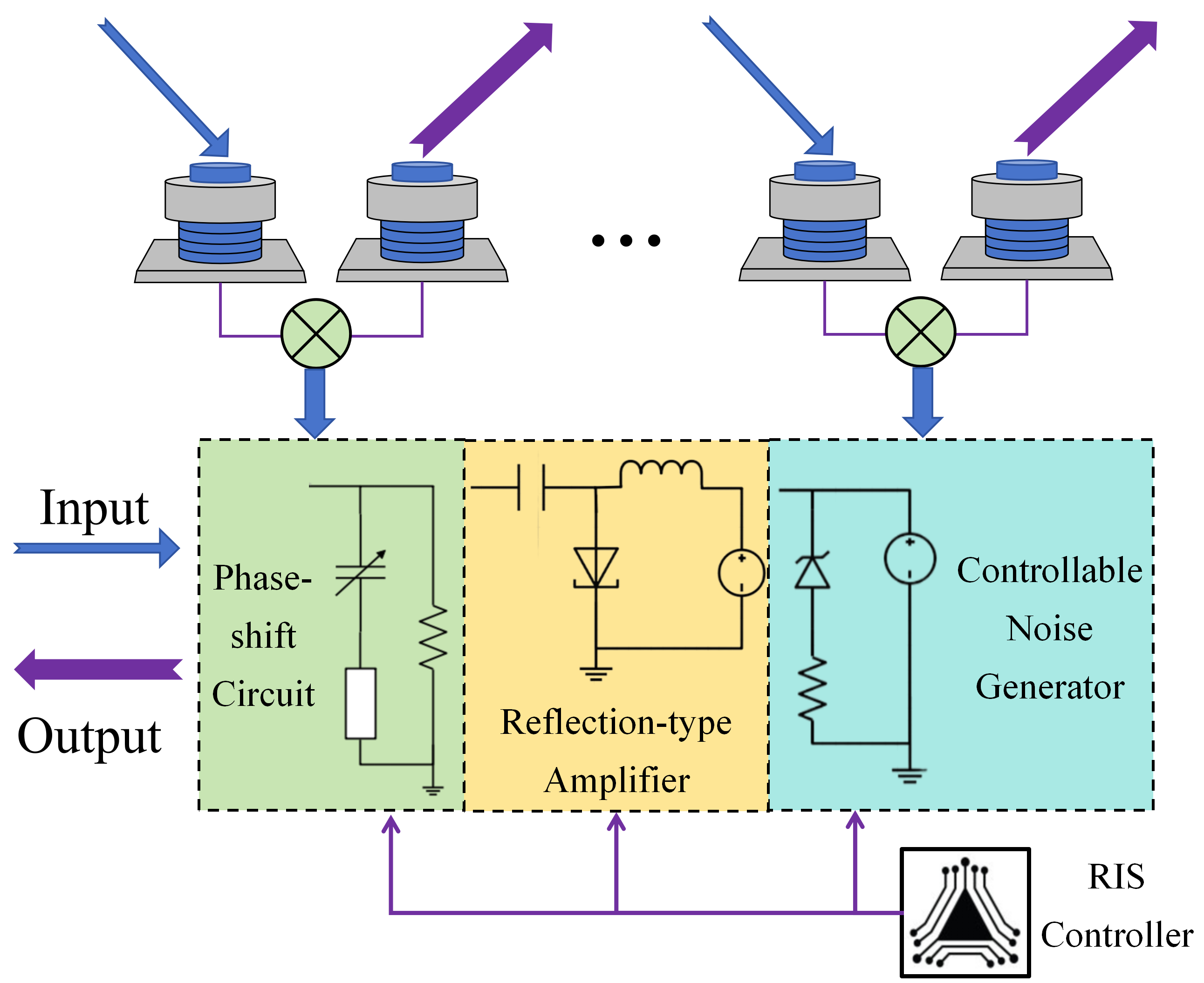
The UARIS enhances underwater communication by absorbing and radiating sound waves, with its working mechanism summarized as ”absorption first, radiation later.” Specifically, each reflection unit of the UARIS consists of two piezoelectric elements. When sound waves impinge on the surface of the acoustic UARIS, the piezoelectric elements first absorb the acoustic energy and adjust the phase and amplitude of the reflected sound waves through internal circuits. The adjusted sound waves are then radiated by another piezoelectric element, thereby achieving intelligent control of the sound waves. Additionally, each reflection unit is integrated with a reflection-type power amplifier, allowing the UARIS to amplify the signal while reflecting it, thus overcoming the attenuation of underwater acoustic signals. This active feature not only effectively improves the quality and SNR of the communication signal but also enables the protection of the SN’s location privacy by adding AN.

With the support of the existing UARIS architecture, the reflected and amplified signals of the $M$-element UARIS can be formulated as follows:

where $\mathbf{\Theta}$ represents the reflection coefficient matrix of the UARIS, in which $p_{m}\in\mathbb{R}_{+}$ and $\theta_{m}$ denote the amplification factor and the phase shift factor of element $m$. Meanwhile, the active characteristics of UARIS introduce corresponding noise, which can be categorized into dynamic noise $\mathbf{\Theta}\mathbf{v}$ and static noise $\mathbf{n_{s}}$. Specifically, $\mathbf{v}$ is related to the input noise of UARIS and the inherent device noise, while $\mathbf{n_{s}}$ mainly represents the noise generated by the phase shift circuit. Since the energy of $\mathbf{n_{s}}$ is extremely small compared to $\mathbf{\Theta}\mathbf{v}$, $\mathbf{n_{s}}$ is neglected in the subsequent analysis.

Additionally, the noise generated at the UARIS can be considered the AN to interfere with the ENs [22]. To further protect the location privacy of the SN, we introduce a controllable noise generator to dynamically adjust the AN introduced at the UARIS, of which the architecture is shown in Fig. 2. Specifically, based on the structure shown in Fig. 2, we can model the AN $\mathbf{v}$ as $\mathbf{v}\sim\mathcal{CN}(\mathbf{0}_{M},\eta\sigma_{v}^{2}\mathbf{I}_{M})$, wherein $\eta$ denotes the noise factor of the AN generated at the UARIS.

In this work, the primary research scenario is the acoustic propagation environment in shallow water areas. Different from wireless communications, the unique characteristics of underwater acoustic channels make the study of underwater signal transmission more complex and challenging. The attenuation pattern of underwater acoustic signals with respect to distance $d$ and frequency $f$ can be modeled as

where $\epsilon$ denotes the propagation factor. According to [23], the absorption coefficient $\upsilon(f)$ can be obtained using Thorp’s formula, which is formulated as

In this subsection, we will provide a detailed introduction to the application scenarios of UARIS-assisted UAC enhancement. Specifically, we consider a downlink UAC scenario and denote the symbol vector transmitted to $K$ RNs as $\mathbf{q}:=\left[q_{1},q_{2},\cdots,q_{K}\right]^{\top}\in\mathbb{C}^{K\times 1}$, which satisfies $\mathbb{E}\left\{\mathbf{q}\mathbf{q}^{\dagger}\right\}=\mathbf{I}_{K}$. As shown in Fig. 1 , let $\mathbf{h}_{k}\in\mathbb{C}^{T\times 1}$, $\mathbf{H}\in\mathbb{C}^{M\times T}$ and $\mathbf{g}_{k}\in\mathbb{C}^{M\times 1}$ denote the channel matrix between the SN and RN $k$, that between the SN and the UARIS and that between the UARIS and RN $k$. Then, according to (1a), signal $b_{k}\in\mathbb{C}$ received at RN $k$ can be modeled as

where $\mathbf{w}_{k}\in\mathbb{C}^{T\times 1}$ denotes the beamforming vector designed by the SN for symbol $q_{k}$. Additionally, $\mathbf{g}_{k}^{\dagger}\mathbf{\Theta}\mathbf{v}$ denotes the AN introduced by the UARIS, while $n_{k}$ denote the background noise introduced at RN $k$, with $n_{k}\sim\mathcal{CN}(0,\sigma^{2})$.

This subsection will introduce modeling the signals received by ENs in a shallow water environment. Specifically, assume that $J$ ENs possess spatial diversity and time synchronization characteristics, and each EN is equipped with an omni-directional hydrophone. Meanwhile, each EN records the received acoustic signals at predetermined observation intervals, then producing $N$ samples after sampling and baseband conversion. In addition, the scope of this work focuses on (approximately) constant-velocity environments and high-frequency signals, where the straight-line model is approximately valid.

Based on the three-ray model in [24], we added a transmission path through the UARIS, thus forming the four-ray model for shallow water transmission, illustrated in Fig. 1. In this model, the four signal transmission paths are respectively:

1. 1.

   $L_{1j}$: The direct LOS path;

2. 2.

   $L_{2j}$: The sea surface reflected NLOS path;

3. 3.

   $L_{3j}$: The seabed reflected NLOS path;

4. 4.

   $L_{4j}$: The UARIS reflected NLOS path.

According to Fig. 1, the corresponding distances of these four paths can be further obtained, which are given by

where $h$ denotes the depth of the seabed, and $l_{j}(\mathbf{p}_{S})$ represents the horizontal distance between the SN and EN $j$, which is defined as $l_{j}(\mathbf{p}_{S})=\sqrt{(x_{S}-x_{j})^{2}+(y_{S}-y_{j})^{2}}$. We can further obtain the transmission delays for each path as follows:

where $c$ represents the sound speed in shallow water.

Formally, the frequency domain representation $\mathbf{{u}}_{j}=\left[{u}_{j}[1],\cdots,{u}_{j}[N]\right]^{\top}\in\mathbb{C}^{N\times 1}$ of the sampled baseband-converted signal obtained from EN $j$ can be modeled as

where $\mathbf{{s}}=\left[{s}[1],\cdots,{s}[N]\right]^{\top}\in\mathbb{C}^{N\times 1}$ denotes the frequency domain representation of the signal transmitted by the SN and $\omega_{n}=2\pi(n-1)/(NT_{s})$ represents the angular frequency of the $k$-th frequency component. Additionally, let $\mathbf{h}_{E,j}\in\mathbb{C}^{T\times 1}$ and $\mathbf{g}_{E,j}\in\mathbb{C}^{M\times 1}$ denote the channel matrix between the SN and EN $j$, and that between the UARIS and EN $j$. Then, the noise ${v}_{j}[n]$ can be denoted as

where ${v}_{0}[n]$ is the background noise which satisfies ${v}_{0}[n]\sim\mathcal{CN}(0,\sigma^{2})$. Meanwhile, we can obtain the attenuation coefficients ${f_{ij}}$, which can be formulated as

where $\kappa_{b}$ is the seabed reflection coefficient.

For shorthand, we further define

According to 10, we can further simplify 7 as

To more accurately reflect the eavesdropping issue in a shallow open-sea environment, we assume the EN has no access to any information about the SN. Specifically, the EN has no prior knowledge of the channel matrix $\mathbf{F}\triangleq\left[\mathbf{f}_{1},\cdots,\mathbf{f}_{J}\right]\in\mathbb{C}^{4\times J}$ or the signal waveform transmitted by the SN. The EN only knows the seabed depth $h$ and the sound speed $c$. Without of generality, we can further assume that $\|{s}\|_{2}=1,$ viz., ${s}\in\mathcal{S}_{N}\triangleq\left\{z\in\mathbb{C}^{N\times 1}:\|z\|_{2}=1\right\}$, where $S_{N}$ denotes the $N$-dimensional unit sphere [24].

The solution of the SBL method can be regarded as the Maximum Likelihood Estimate (MLE) of $\mathbf{p}$, obtained through the joint estimation of all unknown deterministic model parameters. In this case, the maximum likelihood value of $\mathbf{p}$ is the solution to a nonlinear least squares problem:

Different from other traditional shallow sea localization methods, the SBL method we employ introduces some additional computational complexity but is more suited to practical eavesdropping localization scenarios and offers higher robustness. The method is summarized in Algorithm 1, of which further analysis can be obtained in [24].

In this subsection, we primarily analyze the Cramér-Rao Lower Bound (CRLB) for the SBL method. Specifically, without loss of generality, we focus on analyzing a spectrally flat waveform ${\mathbf{s}}$ [24]. Therefore, $s[n]=\frac{1}{\sqrt{N}}e^{\jmath\varphi[n]}$ for all $n$, which means that the ENs can directly estimate the phase of the unknown source signal waveform. Meanwhile, since the EN also needs to estimate the unknown channel attenuation coefficient, the phase parameters to be estimated have only $N-1$ degrees of freedom, that is, the ENs only need to estimate $\boldsymbol{\varphi}\triangleq\left[\varphi[2],\cdots,\varphi[N]\right]^{\top}\in\mathbb{R}^{(N-1)\times 1}$.

To facilitate further derivation, we additionally define $\overline{\mathbf{u}}\triangleq[\mathbf{u}_{1}\cdots\mathbf{u}_{J}]^{\top}\in\mathbb{C}^{NJ\times 1}$, $\overline{\mathbf{G}}\triangleq[\mathbf{G}_{1}\cdots\mathbf{G}_{J}]^{\top}\in\mathbb{C}^{NJ\times N}$, and $\overline{\mathbf{v}}\triangleq[\mathbf{v}_{1}\cdots\mathbf{v}_{J}]^{\top}\in\mathbb{C}^{NJ\times 1}$. Thus, (11) can be rewritten as

Furthermore, according to (8), we can obtain that $v_{j}[n]\sim\mathcal{CN}\left(0,\mathbf{g}_{E,j}^{\dagger}\mathbf{\Theta}\mathbf{\Theta}^{\dagger}\mathbf{g}_{E,j}\eta\sigma_{v}^{2}\right)$. Denoting $\boldsymbol{\sigma}^{2}_{v}\triangleq\eta\sigma_{v}^{2}\boldsymbol{\Gamma}\triangleq\eta\sigma_{v}^{2}\left[\Gamma_{v_{1}}\cdots\Gamma_{v_{J}}\right]^{\top}\in\mathbb{R}^{J\times 1}_{+}$, wherein $\Gamma_{v_{j}}=\mathbf{g}_{E,j}^{\dagger}\mathbf{\Theta}\mathbf{\Theta}^{\dagger}\mathbf{g}_{E,j}+\sigma^{2}/(\eta\sigma_{v}^{2})$, it follows that

Thus, we can calculate the Fisher information matrix (FIM) elements for the Complex Normal (CN) signal model $\overline{\mathbf{u}}$, which can be formulated as [26]

where let $\boldsymbol{\vartheta}$ denote the vector of all unknown deterministic parameters that the ENs need to estimate, which is defined as

where $N_{\vartheta}=3+(N-1)+2\times 4J+J$ represents the number of parameters to be estimated, and we define $\mathbf{J}(\boldsymbol{\vartheta})$ as the FIM.

In the received signal model of the ENs, the parameters to be estimated differ between the mean vector and the covariance matrix. Therefore, we can further deduce that

namely the FIM has a block diagonal structure. Consequently, the elements in $\mathbf{J}(\boldsymbol{\vartheta})$ corresponding to the estimated parameters related to the signal model can be calculated as

To obtain the complete FIM, we also need to compute the derivative of $\overline{\mathbf{G}}\mathbf{s}$ with respect to the parameters $\boldsymbol{\vartheta}$, which can be formulated as for all $i\in\{1,\cdots,4\}$, $j\in\mathcal{J}$, and $\vartheta_{p}\in\{x_{p},y_{p},z_{p}\}$

By substituting (23)-(26) into (22), the complete FIM $\mathbf{J}(\boldsymbol{\vartheta})$ can be computed. Furthermore, according to (22), it can be observed that the FIM block related to the signal components is inversely proportional to the noise $\eta\sigma_{v}^{2}$ introduced by the UARIS. Therefore, the CRLB block associated with the signal components is directly proportional to $\eta\sigma_{v}^{2}$. Finally, the CRLB for this signal estimation model can be given by

According to the underwater communication model in (4), the signal-to-interference-plus-noise ratio (SINR) at RN $k$ can be calculated as

where $\overline{\mathbf{h}}_{k}^{\dagger}=\mathbf{h}_{k}^{\dagger}+\mathbf{g}_{k}^{\dagger}\mathbf{\Theta}\mathbf{H}\in\mathbb{C}^{1\times T}$ represents the equivalent channel vector between the SN and RN $k$.

Furthermore, to jointly optimize the UARIS-assisted communication enhancement and location privacy protection, we formulate the following optimization problem:

where $\mathbf{w}\triangleq\left[\mathbf{w}_{1}^{\top},\cdots,\mathbf{w}_{K}^{\top}\right]^{\top}\in\mathbb{C}^{TK\times 1}$.

According to the CRLB analysis in Subsection IV-B, since the $\sum_{i=1}^{3}|\mathrm{CRLB}(\boldsymbol{\vartheta})_{i,i}|$ is directly proportional to the controllable noise $\eta\sigma_{v}^{2}$ introduced by the UARIS, the optimization problem (29) can be reformulated as

where $\xi$ represents the weight parameter that balances communication enhancement and location privacy protection, and we further define $\xi=\xi_{0}/K\ll 1$. Moreover, for sufficiently large $\gamma_{k}$ and $1/\eta\sigma_{v}^{2}$, $\log_{2}\left[\frac{1+\gamma_{k}}{(1+1/\eta\sigma_{v}^{2})^{\xi}}\right]$ can be approximated by $\log_{2}\left[1+\gamma_{k}(\eta\sigma_{v}^{2})^{\xi}\right]$. Thus, the optimization problem (30) can be reformulated as

The non-convexity of (31) makes it challenging to solve directly. To handle this non-convex logarithmic and fractional problem, we employ the Fractional Programming (FP) method to decouple (31), enabling the optimization of multiple variables separately. Therefore, the following lemma needs to be introduced [27]:

$\mathit{Proof.}$ Detailed proof can be found in [27].

Based on Lemma 1, the original joint optimization problem can be decoupled into an alternate optimization of the SN beamforming vector $\mathbf{w}$, UARIS reflection matrix $\boldsymbol{\Theta}$, noise factor $\eta$, auxiliary variables $\boldsymbol{\zeta}$ and $\boldsymbol{\chi}$. According to [27], if all variables in Problem 1 are optimal in each iteration update, a locally optimal solution to (32) can be obtained after convergence. Therefore, we will provide a detailed introduction to the optimization steps for each variable, and summarize the proposed joint optimization scheme in Algorithm 2.

1. 1.

   Optimize $\boldsymbol{\zeta}$: Fix variables $\left(\mathbf{w},\boldsymbol{\Theta},\eta,\boldsymbol{\chi}\right)$, and optimize auxiliary variables $\boldsymbol{\zeta}$ as

   $$\zeta_{k}^{op}=\frac{|\overline{\mathbf{h}}_{k}^{\dagger}\mathbf{w}_{k}|^{2}(\eta\sigma_{v}^{2})^{\xi}}{\sum_{a=1}^{K}|\overline{\mathbf{h}}_{k}^{\dagger}\mathbf{w}_{a}|^{2}+\left\|\mathbf{g}_{k}^{\dagger}\mathbf{\Theta}\right\|^{2}\eta\sigma_{v}^{2}+\sigma^{2}},$$

   (33)

2. 2.

   Optimize $\boldsymbol{\chi}$: Fix variables $\left(\mathbf{w},\boldsymbol{\Theta},\eta,\boldsymbol{\zeta}\right)$, and optimize auxiliary variables $\boldsymbol{\chi}$ by solving $\partial R_{4}/\partial\chi_{k}=0$ as

   $$\chi_{k}^{op}=\frac{\sqrt{(\eta\sigma_{v}^{2})^{\xi}(1+\zeta_{k})}\overline{\mathbf{h}}_{k}^{\dagger}\mathbf{w}_{k}}{\sum_{a=1}^{K}|\overline{\mathbf{h}}_{k}^{\dagger}\mathbf{w}_{a}|^{2}+\left\|\mathbf{g}_{k}^{\dagger}\mathbf{\Theta}\right\|^{2}\eta\sigma_{v}^{2}+\sigma^{2}},$$

   (34)

3. 3.

   Optimize $\eta$: Fix variables $\left(\mathbf{w},\boldsymbol{\Theta},\boldsymbol{\zeta},\boldsymbol{\chi}\right)$, and optimize the noise factor $\eta$ by solving $\partial R_{4}/\partial\eta=0$ as

   	$\displaystyle\eta^{*}=\left(\frac{2}{\xi}\frac{\sum_{k=1}^{K}|\chi_{k}|^{2}\left\|\mathbf{g}_{k}^{\dagger}\mathbf{\Theta}\right\|^{2}\sigma_{v}^{2}}{\sum_{k=1}^{K}2\sqrt{\sigma_{v}^{2\xi}(1+\zeta_{k})}\mathcal{R}\left\{\chi^{*}\overline{\mathbf{h}}_{k}^{\dagger}\mathbf{w}_{k}\right\}}\right)^{\frac{2}{\xi-2}},$		(35a)
   	$\displaystyle\eta^{op}=\max\left(1,\min\left(\eta^{*},\frac{P_{U}^{\max}-\sum_{k=1}^{K}\|\mathbf{\Theta}\mathbf{G}\mathbf{w}_{k}\|^{2}}{\|\mathbf{\Theta}\|_{F}^{2}\sigma_{v}^{2}}\right)\right)$		(35b)

4. 4.

   Optimize $\mathbf{w}$: For shorthand, we further define

   	$\displaystyle\boldsymbol{\alpha}_{k}\!\!=\!\!\sqrt{(\eta\sigma_{v}^{2})^{\xi}(1\!+\!\zeta_{k})}\chi_{k}\overline{\mathbf{h}}_{k}^{\dagger},\boldsymbol{\alpha}\!\!\triangleq\!\!\left[\boldsymbol{\alpha}_{1}^{\top}\!,\!\cdots\!,\!\boldsymbol{\alpha}_{1}^{\top}\right]^{\top}\!\!\!,$		(36a)
   	$\displaystyle\mathbf{B}\!\!=\!\!\mathbf{I}_{K}\otimes\sum_{k=1}^{K}|\chi_{k}|^{2}\overline{\mathbf{h}}_{k}\overline{\mathbf{h}}_{k}^{\dagger},\mathbf{C}\!\!=\!\!\mathbf{I}_{K}\otimes(\mathbf{H}^{\dagger}\boldsymbol{\Theta}^{\dagger}\boldsymbol{\Theta}\mathbf{H})$		(36b)

   Then, fix variables $\left(\boldsymbol{\Theta},\eta,\boldsymbol{\zeta},\boldsymbol{\chi}\right)$, and obtain a new optimization problem for the SN beamforming vector $\mathbf{w}$ based on (32), which can be formulated as

   	$\displaystyle\mathcal{P}_{5}:\max_{\mathbf{w}}\$	$\displaystyle\mathcal{R}\left\{2\boldsymbol{\alpha}^{\dagger}\mathbf{w}\right\}-\mathbf{w}^{\dagger}\mathbf{B}\mathbf{w},$		(37a)
   	s.t.	$\displaystyle\mathcal{C}_{1}:\|\mathbf{w}\|^{2}\leq P_{S}^{\max},$		(37b)
   		$\displaystyle\mathcal{C}_{2}:\mathbf{w}^{\dagger}\mathbf{C}\mathbf{w}\leq P_{U}^{\max}-\|\mathbf{\Theta}\|_{F}^{2}\eta\sigma_{v}^{2},$		(37c)

   As a standard quadratic constraint quadratic programming, optimization problem (37) can be solved directly using CVX tool to obtain the optimal beamforming vector $\mathbf{w}^{op}$.

5. 5.

   Optimize $\boldsymbol{\Theta}$: For shorthand, we further define

   	$\displaystyle\mathbf{v}=$	$\displaystyle\sum_{k=1}^{K}\sqrt{(\eta\sigma_{v}^{2})^{\xi}(1\!+\!\zeta_{k})}\mathrm{Diag}\left(\boldsymbol{\chi}_{k}^{*}\mathbf{g}_{k}^{\dagger}\right)\mathbf{H}\mathbf{w}_{k}$
   		$\displaystyle-\sum_{k=1}^{K}|\boldsymbol{\chi}_{k}|^{2}\mathrm{Diag}(\mathbf{g}_{k}^{\dagger})\mathbf{H}\sum_{a=1}^{K}\mathbf{w}_{a}\mathbf{w}_{a}^{\dagger}\mathbf{h}_{k},$		(38a)
   	$\displaystyle\boldsymbol{\Lambda}=$	$\displaystyle\sum_{k=1}^{K}|\boldsymbol{\chi}_{k}|^{2}\sum_{j=1}^{K}\mathrm{Diag}\left(\mathbf{g}_{k}^{\dagger}\right)\mathbf{H}\mathbf{w}_{j}\mathbf{w}_{j}^{\dagger}\mathbf{H}^{\dagger}\mathrm{Diag}\left(\mathbf{g}_{k}\right)$
   		$\displaystyle+\sum_{k=1}^{K}|\boldsymbol{\chi}_{k}|^{2}\mathrm{Diag}\left(\mathbf{g}_{k}^{\dagger}\right)\mathrm{Diag}\left(\mathbf{g}_{k}\right)\sigma_{v}^{2},$		(38b)
   	$\displaystyle\boldsymbol{\Psi}=$	$\displaystyle\sum_{k=1}^{K}\mathrm{Diag}(\mathbf{H}\mathbf{w}_{k})\left(\mathrm{Diag}(\mathbf{H}\mathbf{w}_{k})\right)^{\dagger}+\eta\sigma_{v}^{2}\mathbf{I}_{M}.$		(38c)

   Then, fix variables $\left(\mathbf{w},\eta,\boldsymbol{\zeta},\boldsymbol{\chi}\right)$, and obtain a new optimization problem for the UARIS reflection matrix $\boldsymbol{\Theta}$ based on (32), which can be formulated as

   	$\displaystyle\mathcal{P}_{6}:\max_{\boldsymbol{\theta}}\$	$\displaystyle\mathcal{R}\left\{2\boldsymbol{\theta}^{\dagger}\mathbf{v}\right\}-\boldsymbol{\theta}^{\dagger}\boldsymbol{\Lambda}\boldsymbol{\theta},$		(39a)
   	s.t.	$\displaystyle\mathcal{C}_{1}:\boldsymbol{\theta}^{\dagger}\boldsymbol{\Psi}\boldsymbol{\theta}\leq P_{U}^{\max}.$		(39b)

   Furthermore, we use the Lagrange multiplier method to solve optimization problem (39). Specifically, we introduce the Lagrange multiplier $\mu$ and construct the Lagrange function as

   $$\mathcal{L}(\boldsymbol{\theta},\mu)=\mathcal{R}\left\{2\boldsymbol{\theta}^{\dagger}\mathbf{v}\right\}-\boldsymbol{\theta}^{\dagger}\boldsymbol{\Lambda}\boldsymbol{\theta}+\mu(P_{U}^{\max}-\boldsymbol{\theta}^{\dagger}\boldsymbol{\Psi}\boldsymbol{\theta}).$$

   (40)

   Next, take the derivative of the Lagrange function $\mathcal{L}(\boldsymbol{\theta},\mu)$ with respect to $\boldsymbol{\theta}$ and set the derivative to zero:

   $$\frac{\partial\mathcal{L}}{\partial\boldsymbol{\theta}}=2\mathbf{v}-2\boldsymbol{\Lambda}\boldsymbol{\theta}-2\mu\boldsymbol{\Psi}\boldsymbol{\theta}=0.$$

   (41)

   By solving the linear equation system 41, the solution for $\boldsymbol{\theta}$ can be obtained as

   $$\boldsymbol{\theta}=\left(\boldsymbol{\Lambda}+\mu\boldsymbol{\Psi}\right)^{-1}\mathbf{v},$$

   (42)

   wherein the optimal Lagrange multiplier $\mu$ that satisfies power constraint (39b) can be obtained through a binary search [28].

References

- [1] S. A. H. Mohsan, Y. Li, M. Sadiq, J. Liang, and M. A. Khan, “Recent advances, future trends, applications and challenges of internet of underwater things (iout): A comprehensive review,” J. Mar. Sci. Eng., vol. 11, no. 1, p. 124, Dec. 2023.
- [2] A. S. Ghazy, G. Kaddoum, and S. Satinder, “Irs-aided secure reliable underwater acoustic communications,” IEEE Trans. Veh. Technol., Jun. 2024.
- [3] Z. Zhu, Y. Zhou, R. Wang, and F. Tong, “Internet of underwater things infrastructure: A shared underwater acoustic communication layer scheme for real-world underwater acoustic experiments,” IEEE Trans. Aerosp. Electron. Syst., vol. 59, no. 5, pp. 6991–7003, May 2023.
- [4] Y. Cao, W. Shi, L. Sun, and X. Fu, “Channel state information-based ranging for underwater acoustic sensor networks,” IEEE Trans. Wireless Commun., vol. 20, no. 2, pp. 1293–1307, Oct. 2020.
- [5] X. Feng, J. Wang, X. Kuai, M. Zhou, H. Sun, and J. Li, “Message passing-based impulsive noise mitigation and channel estimation for underwater acoustic ofdm communications,” IEEE Trans. Veh. Technol., vol. 71, no. 1, pp. 611–625, Nov. 2021.
- [6] Y. Dong, Z. Chen, Z. Song, Y. Chen, and X. Zhang, “Reconfigurable intelligent surface transmission for data importance classification in underwater acoustic networks with energy holes,” in 2023 IEEE Int. Conf. Signal Process. Commun. Comput., ZHENGZHOU, China, Nov. 2023, pp. 1–4.
- [7] P. Bo, W. Tu, X. Tu, F. Qu, and F.-Y. Wang, “Dual ris-aided parallel intelligence surface for ioamvss: A co-design approach for 3c problems,” IEEE Trans. Intell. Veh., Jan. 2024.
- [8] Y. Han, N. Li, Y. Liu, T. Zhang, and X. Tao, “Artificial noise aided secure noma communications in star-ris networks,” IEEE Wirel. Commun. Lett., vol. 11, no. 6, pp. 1191–1195, Mar. 2022.
- [9] S. Arzykulov, A. Celik, G. Nauryzbayev, and A. M. Eltawil, “Artificial noise and ris-aided physical layer security: Optimal ris partitioning and power control,” IEEE Wirel. Commun. Lett., vol. 12, no. 6, pp. 992–996, Mar. 2023.
- [10] M. A. ElMossallamy, H. Zhang, L. Song, K. G. Seddik, Z. Han, and G. Y. Li, “Reconfigurable intelligent surfaces for wireless communications: Principles, challenges, and opportunities,” IEEE Trans. Cogn. Commun. Netw., vol. 6, no. 3, pp. 990–1002, May 2020.
- [11] C. Huang, A. Zappone, G. C. Alexandropoulos, M. Debbah, and C. Yuen, “Reconfigurable intelligent surfaces for energy efficiency in wireless communication,” IEEE Trans. Wirel. Commun., vol. 18, no. 8, pp. 4157–4170, Jun. 2019.
- [12] K. Liu, Z. Zhang, L. Dai, S. Xu, and F. Yang, “Active reconfigurable intelligent surface: Fully-connected or sub-connected?” IEEE Commun. Lett., vol. 26, no. 1, pp. 167–171, Oct. 2021.
- [13] Z. Zhang, L. Dai, X. Chen, C. Liu, F. Yang, R. Schober, and H. V. Poor, “Active ris vs. passive ris: Which will prevail in 6g?” IEEE Trans. Commun., vol. 71, no. 3, pp. 1707–1725, Dec. 2022.
- [14] H. Wang, Z. Sun, H. Guo, P. Wang, and I. F. Akyildiz, “Designing acoustic reconfigurable intelligent surface for underwater communications,” IEEE Trans. Wireless Commun., vol. 22, no. 12, pp. 8934–8948, Apr. 2023.
- [15] G. Zhang, K. Liu, J. Fu, and S. Sun, “Covariance matrix reconstruction method based on amplitude and phase constraints with application to extend array aperture,” J. Acoust. Soc. Am., vol. 151, no. 5, pp. 3164–3176, May 2022.
- [16] Y. Liu, Y. Wang, C. Chen, and C. Liu, “Unified underwater acoustic localization and sound speed estimation for an isogradient sound speed profile,” IEEE Sens. J., vol. 24, no. 3, pp. 3317–3327, Dec 2023.
- [17] S. Sun, S. Qin, Y. Hao, G. Zhang, and C. Zhao, “Underwater acoustic localization of the black box based on generalized second-order time difference of arrival (gstdoa),” IEEE Trans. Geosci. Remote Sens., vol. 59, no. 9, pp. 7245–7255, Nov. 2020.
- [18] X. Li, Y. Wang, B. Qi, and Y. Hao, “Long baseline acoustic localization based on track-before-detect in complex underwater environments,” IEEE Trans. Geosci. Remote Sens., vol. 61, pp. 1–14, May 2023.
- [19] R. Fan, P. Pan, Z. Jin, Y. Su, and F. Dou, “A secure localization scheme for uwsns based on auv formation cooperative beamforming,” in ICC 2024-IEEE International Conference on Communications, Denver, CO, USA, Aug. 2024, pp. 73–78.
- [20] Z. Liu, B. Zhu, Y. Xie, K. Ma, and X. Guan, “Uav-aided secure communication with imperfect eavesdropper location: Robust design for jamming power and trajectory,” IEEE Trans. Veh. Technol., vol. 73, no. 5, pp. 7276–7286, Dec. 2023.
- [21] K. Hou and S. Zhang, “Optimal beamforming for secure integrated sensing and communication exploiting target location distribution,” IEEE J. Sel. Areas Commun., Aug. 2024.
- [22] B. Lyu, C. Zhou, S. Gong, D. T. Hoang, and Y.-C. Liang, “Robust secure transmission for active ris enabled symbiotic radio multicast communications,” IEEE Trans. Wireless Commun., vol. 22, no. 12, pp. 8766–8780, Apr. 2023.
- [23] F. B. Jensen, W. A. Kuperman, M. B. Porter, H. Schmidt, and A. Tolstoy, Computational ocean acoustics. New York, NY, USA: Springer, 2011.
- [24] A. Weiss, T. Arikan, H. Vishnu, G. B. Deane, A. C. Singer, and G. W. Wornell, “A semi-blind method for localization of underwater acoustic sources,” IEEE Trans. Signal Process., vol. 70, pp. 3090–3106, May 2022.
- [25] A. R. Conn, N. I. Gould, and P. L. Toint, Trust region methods. Philadelphia, Philadelphia, USA: SIAM, 2000.
- [26] S. L. Collier, “Fisher information for a complex gaussian random variable: Beamforming applications for wave propagation in a random medium,” IEEE Trans. Signal Process., vol. 53, no. 11, pp. 4236–4248, Nov. 2005.
- [27] K. Shen and W. Yu, “Fractional programming for communication systems—part i: Power control and beamforming,” IEEE Trans. Signal Process., vol. 66, no. 10, pp. 2616–2630, Mar. 2018.
- [28] S. Boyd, N. Parikh, E. Chu, B. Peleato, J. Eckstein et al., “Distributed optimization and statistical learning via the alternating direction method of multipliers,” Found. Trends Mach. Learn., vol. 3, no. 1, pp. 1–122, Jul. 2011.
- [29] Q. Shi, M. Razaviyayn, Z.-Q. Luo, and C. He, “An iteratively weighted mmse approach to distributed sum-utility maximization for a mimo interfering broadcast channel,” IEEE Trans. Signal Process., vol. 59, no. 9, pp. 4331–4340, Apr. 2011.
- [30] B. Jiang, J. Du, C. Jiang, Z. Han, and M. Debbah, “Underwater searching and multi-round data collection via auv swarms: An energy-efficient aoi-aware mappo approach,” IEEE Internet Things J., vol. 11, no. 7, pp. 12 768–12 782, Nov. 2023.