Issues with AUC and Alternative Metrics

Swaroop Mishra Anjana Arunkumar Chitta Baral

Arizona State University

Investigating the AUC Metric and Proposing Alternatives

Swaroop Mishra Anjana Arunkumar Chitta Baral

Arizona State University

Investigating Issues with the Area Under the Curve Metric and Proposing Solutions

Swaroop Mishra Anjana Arunkumar Chitta Baral

Arizona State University

Investigating the Failure Modes of the AUC metric and Exploring Alternatives for Evaluating Systems in Safety Critical Applications

Swaroop Mishra Anjana Arunkumar Chitta Baral

Arizona State University

Abstract

With the increasing importance of safety requirements associated with the use of black box models, evaluation of selective answering capability of models has been critical. Area under the curve (AUC) is used as a metric for this purpose. We find limitations in AUC; e.g., a model having higher AUC is not always better in performing selective answering. We propose three alternate metrics that fix the identified limitations. On experimenting with ten models, our results using the new metrics show that newer and larger pre-trained models do not necessarily show better performance in selective answering. We hope our insights will help develop better models tailored for safety-critical applications.

1 Introduction

Humans have the capability to gauge how much they know; this leads them to abstain from answering whenever they are not confident about an answer. Such a selective answering capability Kamath et al. (2020); Varshney et al. (2020); Garg and Moschitti (2021) is also essential for machine learning systems, especially in the case of safety critical applications like healthcare, where incorrect answering can result in critically negative consequences.

Area under the curve (AUC) has been used as a metric to evaluate models based on their selective answering capability. AUC involves finding model coverage and accuracy, at various confidence values. MaxProb– maximum softmax probability of models’ predictions– has been used as a strong baseline to decide whether to answer a question or abstain Hendrycks and Gimpel (2016a); Lakshminarayanan et al. (2017); Varshney et al. (2022). However, if Model A has higher AUC than Model B, can we always say that A is better at selective answering and thus better suited for safety critical applications than B?

We experiment across 10 models– ranging from bag-of-words models to pre-trained transformers– and find that a model having higher AUC does not necessarily have a higher selective answering capability. We adversarially attack AUC and find several limitations. These limitations prevent AUC from evaluating the efficacy of models in safety critical applications.

[Uncaptioned image] — Table 1: In each case, AUC ranks Model A as having higher performance than Model B. However, B has higher selective answering capability, as explained in Section 2.1. X axis: Coverage and Y axis: Accuracy.

In pursuit of fixing the limitations, we propose an evaluation metric– ‘DiSCA Score’ i.e. Deployment in Safety Critical Applications. Disaster management is a high-impact and regularly occurring safety critical application. Deployment of Machine Learning systems in disaster management will often be through hand-held devices, such as smartphones, hence requiring light-weight models. Subsequently, we incorporate computation requirements in ‘DiSCA Score’, and propose ‘DiDMA Score’ i.e. Deployment in Disaster Management Applications.

NLP applications in disaster management often involve interaction with users Phengsuwan et al. (2021); Mishra et al. (2022a) whose questions may diverge from a training set, due to rich variations in natural language. We therefore further add the evaluation of abstaining capability on Out-of-Distribution (OOD) datasets as part of the metric and propose ‘NiDMA Score’ i.e. NLP in Disaster Management Applications. Summarily, (i) NiDMA covers interactive NLP applications, (ii) DiDMA is specifically tailored to disaster management but can involve non-interactive NLP applications where OOD data is not frequent, and (iii) DiSCA can be used in any safety critical domain.

Our analysis across ten models sheds light on the strengths and weaknesses of various language models. For example, we observe that newer and larger pre-trained models are not necessarily better in performing selective answering. We also observe that model ranking based on the accuracy metric does not match with their ranking based on selective answering capability, similar to the observations by Mishra and Arunkumar (2021). We hope our insights will bring more attention to developing better models and evaluation metrics for safety-critical applications.

2 Investigating AUC

Experiment Details: Our experiments span over ten different models– Bag-of-Words Sum (BOW-SUM) Harris (1954), Word2Vec Sum (W2V SUM) Mikolov et al. (2013), GloVe Sum (GLOVE SUM) Pennington et al. (2014), Word2Vec CNN (W2V CNN) LeCun et al. (1995), GloVe CNN (GLOVE CNN), Word2Vec LSTM (W2V LSTM) Hochreiter and Schmidhuber (1997), GloVe LSTM (GLOVE LSTM), BERT Base (BERT BASE) Devlin et al. (2018), BERT Large (BERT LARGE) with GELU Hendrycks and Gimpel (2016b) and RoBERTa Large ((ROBERTA LARGE) Liu et al. (2019), in line with recent works Hendrycks et al. (2020); Mishra et al. (2020); Mishra and Arunkumar (2021). We analyze these models over two movie review datasets– (i) SST-2 Socher et al. (2013) that contains short expert movie reviews and (ii) IMDb Maas et al. (2011) which consists of full-length inexpert movie reviews. We train models on IMDb and evaluate on both SST-2 and IMDb. Our intuition behind this is to ensure both IID (IMDb test set) and OOD (SST-2 test set) evaluation.

2.1 Adversarial Attack on AUC:

AUC Tail: Consider a case where A has higher overall AUC and lower accuracy than B, in regions of higher accuracy and lower coverage (Table 1, Case 1). Then, B is better because safety critical applications have a lower tolerance for incorrect answering and so most often will operate in the region of higher accuracy. This is seen in the case of the AUCs of BERT-BASE (A) and BERT-LARGE (B) for the SST-2 dataset ¹¹1See Supplementary Material:DiSCA, NiDMA for more details.

Curve Fluctuations: Another case is when accuracy does not vary in a monotonically decreasing fashion. Even though the model has higher AUC, a non-monotonically decreasing curve shape shows that confidence and correctness of answer are not correlated, making the corresponding model comparatively undesirable (Table 1, Cases 2-6)– this is seen across all models over both datasets, especially at regions of low coverage. The fluctuations for the OOD dataset are more frequent and have higher magnitude for most models ¹.

Plateau Formation: The range of maximum softmax probability values that models associate with predictions varies. For example we see that LSTM models have a wide maxprob range, while transformer models (BERT-LARGE, ROBERTA-LARGE) answer all questions with high maxprob values. In the latter case, model accuracy stays above values of 90% in regions of high coverage; this limited accuracy range forms a plateau in the AUC curve. This plateau is not indicative of model performance as the maxprob values (of incorrect answers) in this region are high and relatively unvarying compared to other models; it is therefore undesirable. Such a plateau also makes it difficult to decide which portion of the AUC curve to ignore and find an operating point, while deploying in disaster management applications (where the tolerance for incorrect answering is low). Plateau formation is acceptable when models answer with low maxprob, either always or in regions of high coverage, irrespective of the level of accuracy (though the range should be limited). However, this acceptable curve condition is not observed in any of the models examined, over both datasets.

3 Alternative Metrics

3.1 DiSCA Score

Let $a$ be the maxprob value when accuracy first drops below 100%. Let $b$ be the lower bound maxprob value which when used as a cutoff for answering questions, results in an accuracy that is the worst possible accuracy admissible by the tolerance level of the domain. Let $n$ represent the number of times the slope of the curve is seen to increase with increasing coverage, and $d_{1},d_{2}$ and $c_{1},c_{2}$ respectively represent the accuracy and maxprob values at the two points where this increase in slope occurs, such that $d_{1}<d_{2}$ and $c_{1}>=c_{2}$ . Let $x$ , $y$ , $z$ represent weights that flexibly define the region of interest depending on application requirements, such that $x+y+z=1$ . $b$ is a hyperparameter; we experiment with a range of $b$ values, where the worst possible accuracy varies from 100% to 50%. The DiSCA Score is defined as:

DiSCA=\frac{x}{a}+\frac{y}{b}-\frac{z\cdot\sum_{i}^{n}(n-i+1)\cdot\frac{(d_{2}-d_{1})}{c}}{\sum_{i}^{n}(n-i+1)}

(1)

where

c=\begin{cases}(c_{1}-c_{2})&\text{if}\ (c_{1}-c_{2})>0.001\\ 0.001&\text{otherwise}\end{cases}

Our definition of $c$ is based on the observation of very low order differences in maxprob values for CNN and transformer models.

3.1.1 Observations:

First Term: From Figure 2(A), we see that the $a$ values are lower for the BERT-BASE, W2V-LSTM and RoBERTA-LARGE models, indicating that the first incorrect classification occurs at lower maxprob values than in other models. Based on equation 1, BERT-BASE, W2V-LSTM and RoBERTA-LARGE are the top-3 models respectively based on the first term of DiSCA Score.

Refer to caption — Figure 1: $b$ for (A)IMDb, (B) SST-2 datasets. Values from 1-0.5 on the x-axis represent the accuracy thresholds considered, while ‘Lowest Maxprob’ represents the lowest maxprob value a model assigns at 100% coverage.

MODEl	<0.95	<0.90	<0.85	<0.80	<0.75	<0.70	<0.65	<0.60	<0.55
BERT-BASE	0.69	0.69	0.69	0.69	0.69	0.69	0.69	0.69	0.69
W2V-LSTM	0.63	0.65	0.65	0.65	0.65	0.65	0.65	0.65	0.65
GLOVE-CNN	0.54	0.54	0.54	0.54	0.54	0.54	0.54	0.54	0.54
GLOVE-SUM	0.52	0.54	0.56	0.56	0.56	0.56	0.56	0.56	0.56
BERT-LARGE	0.48	0.48	0.48	0.48	0.48	0.48	0.48	0.48	0.48
ROBERTA-LARGE	0.45	0.45	0.45	0.45	0.45	0.45	0.45	0.45	0.45
GLOVE-LSTM	0.37	0.37	0.37	0.37	0.37	0.37	0.37	0.37	0.37
W2V-SUM	0.35	0.37	0.39	0.39	0.39	0.39	0.39	0.39	0.39
W2V-CNN	0.36	0.36	0.36	0.36	0.36	0.36	0.36	0.36	0.36
BOW-SUM	-6.71	-6.71	-6.71	-6.71	-6.71	-6.71	-6.71	-6.71	-6.71

MODEL	<0.95	<0.90	<0.85	<0.80	<0.75	<0.70	<0.65	<0.60	<0.55
W2V-SUM	0.71	0.71	0.71	0.71	0.71	0.71	0.71	0.71	0.71
GLOVE-LSTM	0.65	0.67	0.70	0.70	0.70	0.70	0.70	0.70	0.70
GLOVE-SUM	0.60	0.61	0.63	0.65	0.68	0.68	0.68	0.68	0.68
BERT-LARGE	0.60	0.62	0.62	0.62	0.62	0.62	0.62	0.62	0.62
BERT-BASE	0.43	0.45	0.45	0.45	0.45	0.45	0.45	0.45	0.45
ROBERTA-LARGE	0.22	0.24	0.24	0.24	0.24	0.24	0.24	0.24	0.24
W2V-CNN	-0.68	-0.66	-0.64	-0.64	-0.64	-0.64	-0.64	-0.64	-0.64
BOW-SUM	-0.71	-0.69	-0.68	-0.66	-0.63	-0.63	-0.63	-0.63	-0.63
GLOVE-CNN	-2.43	-2.43	-2.42	-2.42	-2.42	-2.42	-2.42	-2.42	-2.42
W2V-LSTM	-3.53	-3.53	-3.53	-3.53	-3.53	-3.53	-3.53	-3.53	-3.53

Table 2: (a) LHS: DiSCA (IID)– (IMDb), (b) RHS: DiSCA (OOD)– SST-2;

x

y

z

=0.33. The column header indicates the accuracy threshold used to calculate

b

. Green: Model accuracy falls below the threshold indicated by the column head, but is higher than the next column threshold. Yellow: If the latter is false. White: Model’s overall accuracy is higher than the threshold of that column, and therefore never falls below that threshold.

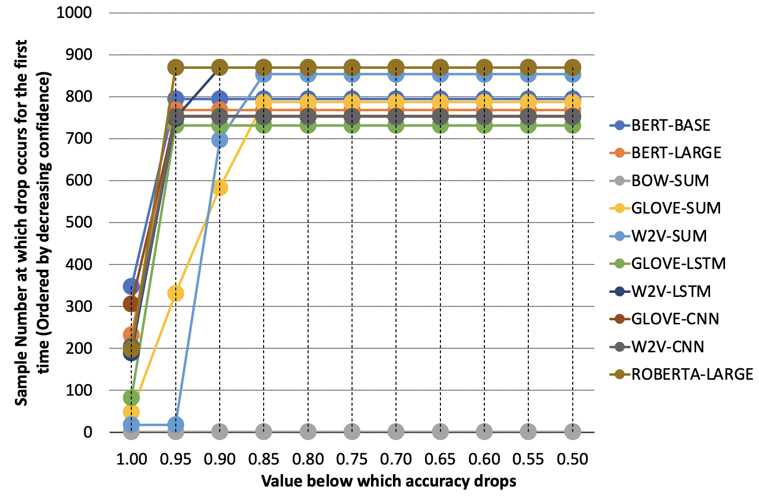
Second Term: Figure 1(A) illustrates the $b$ values of various models, over a range of worst possible accuracies. In RoBERTA-LARGE, when the accuracy drops below 95%, the maxprob value is 0.53; it is above 0.8 for other models. This shows that RoBERTA-LARGE is better than other models for the 90-95% accuracy bin. GLOVE-SUM is found to be relatively better overall, than other models, as its maxprob is a better indicator of accuracy (seen from sharper decrease in the figure). BOW-SUM is the worst model as a significant amount of samples with the highest confidence values are classified incorrectly, causing $b$ for all accuracy bins to be extremely high and relatively uniform.

Third Term: The number of times accuracy increases with increase in coverage is highest for the BOW-SUM model, making it the worst model (Figure 3). Word averaging models (W2V-SUM, BOW-SUM, and GLOVE-SUM) are seen to have a higher number of fluctuations on average; other models have near-zero fluctuations, mostly occurring at the highest maxprob samples ¹. The magnitude-number ratio of fluctuations in RoBERTA-LARGE is high, in comparison to other models.

Overall Ranking: In Table 2(a), BERT-BASE is ranked highest, as it has no fluctuation penalty and also has a lower maxprob value when accuracy first drops below 100% ( $a$ ). Since the magnitude-number fluctuation ratio of BERT-LARGE and RoBERTA-LARGE are higher than that seen for W2V-LSTM, GLOVE-CNN, and GLOVE-SUM, the former are ranked lower. Despite GLOVE-SUM having the overall best maxprob-accuracy correlation, its higher fluctuation number lowers the score. BOW-SUM is seen to be the worst (and only negatively scoring model), in line with observations made across all individual terms.

3.2 DiDMA Score

\normalsize DiDMA=p*DiSCA+q*Computation\_Score

(2)

where

Computation\_Score=\frac{1}{Energy}

DiDMA Score is obtained by summing weighted DiSCA Score ( $p$ )and Computation Score ( $q$ ) based on application requirements (such that $p$ + $q$ =1). In Computation Score, models are scored based on the energy usage. Higher energy usage implies lower computation score. We suggest using equations²²2See Supplementary: DiDMA for more details of a recent work Henderson et al. (2020) for the energy calculation. Since, energy usage is hardware dependent, we do not calculate the term here; it should be calculated based on the device of deployment in disaster management.

3.3 NiDMA Score

NiDMA=u*DiDMA+v*DiSCA(OOD)

(3)

NiDMA Score is obtained by summing weighted DiDMA Score( $u$ ) and DiSCA Score on OOD data ( $v$ ) based on application requirements (where $u$ + $v$ =1). Figure 2(B), 1(B) and 3 (SST-2) illustrate the DiSCA Score on OOD datasets.

From Figure 2(B), we see that first term based ranking of the DiSCA(OOD)Score is not preserved with respect to DiSCA Score in Figure 2(A); $a$ values are lowest for the GLOVE-SUM and W2V-SUM models. We also note that for the $b$ values (Figure 1(B)), W2V-LSTM is the worst model, while GLOVE-SUM remains better overall; BERT-BASE and GLOVE-LSTM perform best for the 85-90% and 80-85% accuracy bins respectively .

while other transformer/embeddings models show higher maxprob values ( $>$ 0.8) at higher coverage. In Figure 3, while there is an increase in the number of accuracy fluctuations, we see that model ranking for the number of times accuracy increases is preserved for most models (except LSTM and CNN). The magnitude decreases for BERT-LARGE, word-averaging, and GLOVE-LSTM. The number-magnitude ratio remains high for RoBERTA-LARGE. We also observe a significant change in ranking from Table 2(b), though BERT-LARGE and RoBERTA-LARGE have similar ranking; W2V-SUM is found to have best overall performance in terms of DiSCA (OOD) Score.

4 Conclusion

We adversarially attack the AUC metric that is commonly used for evaluating selective answering capability of models. We find that a model having higher AUC is not always better in terms of its selective answering capability, and subsequently its efficacy in safety critical applications. We propose three alternate metrics to fix the limitations in AUCs. We experiment across ten models and get various insights regarding strengths ans weakness of models. We hope our work will encourage the development of better models and evaluation metrics focusing on the safety requirements of users while interacting with machine learning models, that is getting increasingly popular in the instruction paradigm Mishra et al. (2022b); Sanh et al. (2021); Mishra et al. (2021); Wei et al. (2021); Parmar et al. (2022); Ouyang et al. (2022).

References

Devlin et al. (2018) Jacob Devlin, Ming-Wei Chang, Kenton Lee, and Kristina Toutanova. 2018. Bert: Pre-training of deep bidirectional transformers for language understanding. arXiv preprint arXiv:1810.04805.
Garg and Moschitti (2021) Siddhant Garg and Alessandro Moschitti. 2021. Will this question be answered? question filtering via answer model distillation for efficient question answering. In Proceedings of the 2021 Conference on Empirical Methods in Natural Language Processing, pages 7329–7346.
Harris (1954) Zellig S Harris. 1954. Distributional structure. Word, 10(2-3):146–162.
Henderson et al. (2020) Peter Henderson, Jieru Hu, Joshua Romoff, Emma Brunskill, Dan Jurafsky, and Joelle Pineau. 2020. Towards the systematic reporting of the energy and carbon footprints of machine learning. arXiv preprint arXiv:2002.05651.
Hendrycks and Gimpel (2016a) Dan Hendrycks and Kevin Gimpel. 2016a. A baseline for detecting misclassified and out-of-distribution examples in neural networks. arXiv preprint arXiv:1610.02136.
Hendrycks and Gimpel (2016b) Dan Hendrycks and Kevin Gimpel. 2016b. Gaussian error linear units (gelus). arXiv preprint arXiv:1606.08415.
Hendrycks et al. (2020) Dan Hendrycks, Xiaoyuan Liu, Eric Wallace, Adam Dziedzic, Rishabh Krishnan, and Dawn Song. 2020. Pretrained transformers improve out-of-distribution robustness. arXiv preprint arXiv:2004.06100.
Hochreiter and Schmidhuber (1997) Sepp Hochreiter and Jürgen Schmidhuber. 1997. Long short-term memory. Neural computation, 9(8):1735–1780.
Kamath et al. (2020) Amita Kamath, Robin Jia, and Percy Liang. 2020. Selective question answering under domain shift. arXiv preprint arXiv:2006.09462.
Korukonda et al. (2016) Meher Preetam Korukonda, Swaroop Ranjan Mishra, Anupam Shukla, and Laxmidhar Behera. 2016. Improving microgrid voltage stability through cyber-physical control. In 2016 National Power Systems Conference (NPSC), pages 1–6. IEEE.
Lakshminarayanan et al. (2017) Balaji Lakshminarayanan, Alexander Pritzel, and Charles Blundell. 2017. Simple and scalable predictive uncertainty estimation using deep ensembles. In Advances in neural information processing systems, pages 6402–6413.
LeCun et al. (1995) Yann LeCun, Yoshua Bengio, et al. 1995. Convolutional networks for images, speech, and time series. The handbook of brain theory and neural networks, 3361(10):1995.
Liu et al. (2019) Yinhan Liu, Myle Ott, Naman Goyal, Jingfei Du, Mandar Joshi, Danqi Chen, Omer Levy, Mike Lewis, Luke Zettlemoyer, and Veselin Stoyanov. 2019. Roberta: A robustly optimized bert pretraining approach. arXiv preprint arXiv:1907.11692.
Maas et al. (2011) Andrew L Maas, Raymond E Daly, Peter T Pham, Dan Huang, Andrew Y Ng, and Christopher Potts. 2011. Learning word vectors for sentiment analysis. In Proceedings of the 49th annual meeting of the association for computational linguistics: Human language technologies-volume 1, pages 142–150. Association for Computational Linguistics.
Mikolov et al. (2013) Tomas Mikolov, Ilya Sutskever, Kai Chen, Greg S Corrado, and Jeff Dean. 2013. Distributed representations of words and phrases and their compositionality. In Advances in neural information processing systems, pages 3111–3119.
Min et al. (2021) Sewon Min, Jordan Boyd-Graber, Chris Alberti, Danqi Chen, Eunsol Choi, Michael Collins, Kelvin Guu, Hannaneh Hajishirzi, Kenton Lee, Jennimaria Palomaki, et al. 2021. Neurips 2020 efficientqa competition: Systems, analyses and lessons learned. In NeurIPS 2020 Competition and Demonstration Track, pages 86–111. PMLR.
Mishra and Arunkumar (2021) Swaroop Mishra and Anjana Arunkumar. 2021. How robust are model rankings: A leaderboard customization approach for equitable evaluation. In Proceedings of the AAAI Conference on Artificial Intelligence, volume 35, pages 13561–13569.
Mishra et al. (2020) Swaroop Mishra, Anjana Arunkumar, Chris Bryan, and Chitta Baral. 2020. Our evaluation metric needs an update to encourage generalization. arXiv preprint arXiv:2007.06898.
Mishra et al. (2022a) Swaroop Mishra, Manas Kumar Jena, and Ashok Kumar Tripathy. 2022a. Towards the development of disaster management tailored machine learning systems. In 2022 IEEE India Council International Subsections Conference (INDISCON), pages 1–6. IEEE.
Mishra et al. (2021) Swaroop Mishra, Daniel Khashabi, Chitta Baral, Yejin Choi, and Hannaneh Hajishirzi. 2021. Reframing instructional prompts to gptk’s language. ACL Findings.
Mishra et al. (2022b) Swaroop Mishra, Daniel Khashabi, Chitta Baral, and Hannaneh Hajishirzi. 2022b. Cross-task generalization via natural language crowdsourcing instructions. In Proceedings of the 60th Annual Meeting of the Association for Computational Linguistics (Volume 1: Long Papers), pages 3470–3487.
Mishra and Sachdeva (2020) Swaroop Mishra and Bhavdeep Singh Sachdeva. 2020. Do we need to create big datasets to learn a task? In Proceedings of SustaiNLP: Workshop on Simple and Efficient Natural Language Processing, pages 169–173.
Mishra et al. (2019) Swaroop Ranjan Mishra, Meher Preetam Korukonda, Laxmidhar Behera, and Anupam Shukla. 2019. Enabling cyber-physical demand response in smart grids via conjoint communication and controller design. IET Cyber-Physical Systems: Theory & Applications, 4(4):291–303.
Mishra et al. (2015) Swaroop Ranjan Mishra, N Venkata Srinath, K Meher Preetam, and Laxmidhar Behera. 2015. A generalized novel framework for optimal sensor-controller connection design to guarantee a stable cyber physical smart grid. In 2015 IEEE 13th International Conference on Industrial Informatics (INDIN), pages 424–429. IEEE.
Ouyang et al. (2022) Long Ouyang, Jeff Wu, Xu Jiang, Diogo Almeida, Carroll L Wainwright, Pamela Mishkin, Chong Zhang, Sandhini Agarwal, Katarina Slama, Alex Ray, et al. 2022. Training language models to follow instructions with human feedback. arXiv preprint arXiv:2203.02155.
Parmar et al. (2022) Mihir Parmar, Swaroop Mishra, Mirali Purohit, Man Luo, M Hassan Murad, and Chitta Baral. 2022. In-boxbart: Get instructions into biomedical multi-task learning. NAACL Findings.
Pennington et al. (2014) Jeffrey Pennington, Richard Socher, and Christopher D Manning. 2014. Glove: Global vectors for word representation. In Proceedings of the 2014 conference on empirical methods in natural language processing (EMNLP), pages 1532–1543.
Phengsuwan et al. (2021) Jedsada Phengsuwan, Tejal Shah, Nipun Balan Thekkummal, Zhenyu Wen, Rui Sun, Divya Pullarkatt, Hemalatha Thirugnanam, Maneesha Vinodini Ramesh, Graham Morgan, Philip James, et al. 2021. Use of social media data in disaster management: a survey. Future Internet, 13(2):46.
Sanh et al. (2021) Victor Sanh, Albert Webson, Colin Raffel, Stephen Bach, Lintang Sutawika, Zaid Alyafeai, Antoine Chaffin, Arnaud Stiegler, Arun Raja, Manan Dey, et al. 2021. Multitask prompted training enables zero-shot task generalization. In International Conference on Learning Representations.
Socher et al. (2013) Richard Socher, Alex Perelygin, Jean Wu, Jason Chuang, Christopher D Manning, Andrew Y Ng, and Christopher Potts. 2013. Recursive deep models for semantic compositionality over a sentiment treebank. In Proceedings of the 2013 conference on empirical methods in natural language processing, pages 1631–1642.
Strubell et al. (2019) Emma Strubell, Ananya Ganesh, and Andrew McCallum. 2019. Energy and policy considerations for deep learning in nlp. arXiv preprint arXiv:1906.02243.
Su et al. (2022) Hongjin Su, Jungo Kasai, Chen Henry Wu, Weijia Shi, Tianlu Wang, Jiayi Xin, Rui Zhang, Mari Ostendorf, Luke Zettlemoyer, Noah A Smith, et al. 2022. Selective annotation makes language models better few-shot learners. arXiv preprint arXiv:2209.01975.
Treviso et al. (2022) Marcos Treviso, Tianchu Ji, Ji-Ung Lee, Betty van Aken, Qingqing Cao, Manuel R Ciosici, Michael Hassid, Kenneth Heafield, Sara Hooker, Pedro H Martins, et al. 2022. Efficient methods for natural language processing: A survey. arXiv preprint arXiv:2209.00099.
Varshney et al. (2020) Neeraj Varshney, Swaroop Mishra, and Chitta Baral. 2020. It’s better to say" i can’t answer" than answering incorrectly: Towards safety critical nlp systems. arXiv preprint arXiv:2008.09371.
Varshney et al. (2022) Neeraj Varshney, Swaroop Mishra, and Chitta Baral. 2022. Investigating selective prediction approaches across several tasks in iid, ood, and adversarial settings. In Findings of the Association for Computational Linguistics: ACL 2022, pages 1995–2002.
Wei et al. (2021) Jason Wei, Maarten Bosma, Vincent Zhao, Kelvin Guu, Adams Wei Yu, Brian Lester, Nan Du, Andrew M Dai, and Quoc V Le. 2021. Finetuned language models are zero-shot learners. In International Conference on Learning Representations.

Appendix A DiSCA

Please refer to Figures 4,5,6,7,8,9, 16(A).

Appendix B DiDMA

Equation for Computation Score Henderson et al. (2020):

e_{total}=PUE\sum_{p}(p_{dram}e_{dram}+p_{cpu}e_{cpu}+p_{gpu}e_{gpu})

(4)

where $p_{resource}$ are the percentages of each system resource used by the attributable processes relative to the total in-use resources and $e_{resource}$ is the energy usage of that resource. The same constant power usage effectiveness (PUE) as Strubell et al. (2019) is used. This value compensates for excess energy from cooling or heating the data-center.

Alternatively, computation score can be calculated as the ratio of a fixed ‘optimal’ parameter number (based on the hardware used in deployment) to the number of parameters in the model considered. For example, if a deployment device functions effectively when models with up to 1 million parameters are utilized, a model with 2 million parameters will be assigned a score of 0.5 and one with 500,000 parameters will be assigned a score of 2.

Other efficiency based evaluation in terms of data Mishra and Sachdeva (2020); Su et al. (2022) or model Min et al. (2021); Treviso et al. (2022) can be incorporated in this metric as part of this parameter in future.

Appendix C N-DiDMA

Please refer to Figures 10, 11, 12, 13, 14, 15, 16(B).

N-DiDMA and DiDMA are narrower in scope as they are specific to NLP and disaster management applications whereas DiSCA can be applied in general in any safety-critical applications, for example the cyber-physical smart grid Mishra et al. (2015); Korukonda et al. (2016); Mishra et al. (2019).

Appendix D Infrastructure Used

All the experiments were conducted on ”TeslaV100-SXM2-16GB”; CPU cores per node 20; CPU memory per node: 95,142 MB; CPU memory per core: 4,757 MB. This configuration is not a necessity for these experiments as we ran our operations with NVIDIA Quadro RTX 4000 as well with lesser memory.