(eccv) Package eccv Warning: Package ‘hyperref’ is loaded with option ‘pagebackref’, which is *not* recommended for camera-ready version
Is user feedback always informative?
Retrieval Latent Defending for Semi-Supervised Domain Adaptation without Source Data
Abstract
This paper aims to adapt the source model to the target environment, leveraging small user feedback (i.e., labeled target data) readily available in real-world applications. We find that existing semi-supervised domain adaptation (SemiSDA) methods often suffer from poorly improved adaptation performance when directly utilizing such feedback data, as shown in Figure 1. We analyze this phenomenon via a novel concept called Negatively Biased Feedback (NBF), which stems from the observation that user feedback is more likely for data points where the model produces incorrect predictions. To leverage this feedback while avoiding the issue, we propose a scalable adapting approach, Retrieval Latent Defending. This approach helps existing SemiSDA methods to adapt the model with a balanced supervised signal by utilizing latent defending samples throughout the adaptation process. We demonstrate the problem caused by NBF and the efficacy of our approach across various benchmarks, including image classification, semantic segmentation, and a real-world medical imaging application. Our extensive experiments reveal that integrating our approach with multiple state-of-the-art SemiSDA methods leads to significant performance improvements.
Keywords:
Rethinking user-provided feedback Semi-supervised &Source-free domain adaptation Medical image diagnosis
1 Introduction
While deep neural networks have demonstrated remarkable performance in the development domain (i.e., source domain) [23, 15], they often suffer from performance degradation in the deployed domain (i.e., target domain) due to domain shift [17, 78, 72]. To mitigate this issue, domain adaptation (DA) techniques have been introduced [70, 34, 58]. The most common DA tasks include semi-supervised domain adaptation (SemiSDA) and source-free domain adaptation (SFDA). SemiSDA aims to adapt the model given a small amount of labeled target data along with massive unlabeled target data [58, 6, 99, 66]. SFDA conducts adaptation with only target data without accessing source data considering data privacy or memory constraints in edge devices [34, 92, 67].
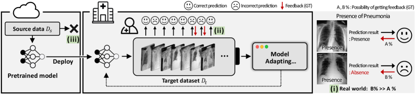
Despite such advances in DA, adapting the model with user feedback still remains an open area for further research, even though practical machine learning (ML) products often allow users to provide feedback in order to further improve the model in the target environment. For example, facial recognition or medical image diagnosis applications enable users to give feedback correcting wrong model predictions, as depicted in Figure 1 (a). Since feedback can be modeled in this case as a small amount of labeled target data, it is anticipated that previous SemiSDA methods assuming the same setup would yield promising results. However, we observe that they show inferior adaptation performance on multiple DA benchmarks when using such user feedback in practice, as shown in the dark-gray bar \makebox(4.0,4.0)[]{{\color[rgb]{0,0,0}\definecolor[named]{pgfstrokecolor}{rgb}{0,0,0}\pgfsys@color@gray@stroke{0}\pgfsys@color@gray@fill{0}~{}~{}}} in Figure 1 (b).

We introduce a novel concept called Negatively Biased Feedback (NBF) to explain this phenomenon. NBF is based on the observation that user feedback is more likely to be derived from incorrect model predictions. For example, a radiologist might log a misdiagnosed chest X-ray by the model, as its accuracy directly impacts the patient’s survival. Interestingly, our observation aligns with findings from cognitive psychology literature [3, 57] that proves that humans are more likely to react and provide feedback to negative events (i.e., wrong model predictions). Since such an NBF scenario is feasible, we analyze its unexpected impact on SemiSDA observed above. We identify that a biased distribution of NBF within the overall data distribution leads to sub-optimal adaptation results, particularly compared to Random Feedback (RF). RF represents the classical SemiSDA setup, where labeled data is randomly selected from the target data.
To address the problem caused by NBF, we present a scalable approach named Retrieval Latent Defending, which can be seamlessly integrated with existing SemiSDA methods. Our approach allows them to adapt the model without a strong dependence on the biasedly distributed labeled data. Specifically, we balance the supervised adapting signal by appending latent defending samples to the mini-batch and help to keep the model’s balanced class discriminability throughout adapting iterations. We evaluate the unexpected influence of NBF using various benchmarks, including image classification, semantic segmentation, and medical image diagnosis. Building upon these evaluations, we demonstrate that our approach not only complements, but significantly enhances the performance of multiple SemiSDA methods.
The contributions of the paper are as follows:
-
We introduce the novel concept called Negatively Biased Feedback and uncover that it can lead to sub-optimal adaptation performance of existing SemiSDA methods.
-
We analyze this problem and present a scalable solution, Retrieval Latent Defending, that combines with SemiSDA methods and allows them to avoid the unexpected effect of NBF.
-
We show that our approach generalizes through diverse DA benchmarks and improves adaptation results of state-of-the-art SemiSDA methods.
-
We publicly release the code on https://github.com/junha1125/RLD-SemiSDA.
2 Related Work
Adaptation in the deployment environment.
Real-world ML products often encounter performance degradation caused by gaps between the source and target environment [17]. One solution is to adapt the model using unlabeled data observed in the target domain, referred to as unsupervised domain adaptation (UDA) [72, 59, 37]. Works on UDA use both source and target data to improve the target performance by using methods such as domain discrepancy minimization by adversarial training [41, 70, 76, 18, 73, 72, 59], and self-training with pseudo labels [45, 98, 51, 97]. Source-free DA (SFDA) builds on UDA and imposes an additional constraint that the source data can not be accessed during domain adaptation. This has practical implications for addressing data privacy concerns or barriers in data transmission to edge devices [34, 38, 77, 95]. The majority of recent SFDA works rely on strategies like domain clustering [34], nearest neighbors [92, 93, 91], and contrastive learning [8, 35, 101]. Nevertheless, SFDA does not consider the availability of small labeled data, which may be available in practical ML systems. Semi-supervised DA (SemiSDA) works mainly demonstrate that permitting small labeled data in the target domain can substantially enhance adaptation performance compared to traditional UDA [58]. Their primary strategy is to use domain alignment [58, 33, 20, 94], multi-view consistency [33, 6, 2, 89], and asymmetric co-training [36, 90].
Active domain adaptation
(ActiveDA) [55, 86, 25] envisions a scenario in which the machine selects specific target samples and instructs annotators to label them. The primary objective of ActiveDA is to strategically identify and select the most informative samples for annotation. These chosen samples (i.e., labeled target data) are subsequently utilized to update the source model using SemiSDA methods [58, 33], and the effectiveness of ActiveDA is assessed by evaluating the target performance of the adapted model.
Semi-supervised learning
(SemiSL) aims to reduce expensive human annotations, and propose methods to train a model from scratch using massive unlabeled data along with limited amounts of labeled data [74, 43]. The majority of SemiSL methods depend on consistency regularization [60, 66, 87, 5, 4, 16], which helps the model to make similar predictions for augmented versions of the same image. Moreover, adaptive thresholding [66, 81, 24, 88, 12, 9, 99] is also popularly utilized to produce reliable pseudo labels from unlabeled data.
SemiSDA and SemiSL setups mimic small labeled datasets by randomly selecting subsets of the target dataset, whereas ActiveDA involves selections instructed by the machine. In contrast, this paper posits that in real-world applications, labeled data is typically acquired through user intervention. Additionally, users often provide feedback on samples misclassified by the model (i.e., negatively biased feedback), a process detailed in the following section.
| UDA | SFDA | ActiveDA | SemiSDA | SemiSL | Our setup | |
|---|---|---|---|---|---|---|
| Adaptation | ||||||
| Source-free | - | |||||
| Feedback | machine-instructed | randomly selected | randomly selected | user-provided |
The table above summarizes the comparison of relevant studies to our setup. In the table, adaptation means fine-tuning the source pre-trained model (as opposed to training from scratch); feedback represents a small number of labeled target samples. Appendix A provides further comparisons with settings like class-imbalanced SemiSDA and test-time adaptation (TTA).
3 Negatively Biased Feedback
3.1 Adaptation with user feedback.
Our adaptation setup is illustrated in Figure 2. A model is pre-trained on the source data . Next, the model is deployed to the target domain, such as a smartphone or a hospital, where we assume the transfer of is prohibited due to data privacy regulations or resource constraints (same setup as SFDA [34]). While users utilize ML products on the target domain, the model provides prediction results for data observed in the target domain and occasionally obtains user feedback in the form of annotations . We represent the target data as , where , and denote labeled and unlabeled data and and is their number of data. Lastly, the model can utilize and SemiSDA algorithms for adaptation during its inactive phase (e.g., when users do not use the product, like at nighttime) in order to alleviate performance degradation due to domain shift or to personalize the model based on user feedback.

Rethinking user-provided feedback.
Classical SemiSDA works simply assume that a random subset in target data is labeled by users when building . However, as illustrated in Figure 2 , we suggest that users are more likely to provide feedback on misclassified samples by the source model, named negatively biased feedback (NBF). This behavior can be understood from two perspectives: (a) users generally expect their feedback to be used as a basis of model improvement, motivating them to provide NBF, and (b) humans tend to react more strongly to negative experiences, such as receiving incorrect predictions, as observed in psychological studies [3, 57]. We note that the NBF assumption holds more strongly for the medical application: it is reasonable to imagine that the user (i.e., radiologist) logs the mistakes of the model while diagnosing a chest X-ray exam because the diagnostic accuracy of the model is directly related to the patient’s chances of survival. Furthermore, applications beyond the medical domain can also exhibit NBF. For instance, users in self-driving cars can report errors, such as object detection failures or navigation mistakes, to enhance the car’s driving capabilities.
3.2 Influence of NBF on SemiSDA
Simulation study.
As shown in Figure 3, we conduct a simulation study to understand the effect of NBF on SemiSDA. We first use the blobs dataset [53] and construct the source and target data so that domain shift exists between them (left sub-figures). We pre-train a source model on the source data and compute the accuracy in the target domain, where the performance drop due to domain shift is observed (98.5%→76.4%). Next, we simulate two types of feedback (i.e., labeled data): random feedback and negatively biased feedback following a previous SemiSDA setup and our setup, respectively. Specifically, NBF is randomly selected among misclassified samples by the source model. We find that random feedback (RF) points are evenly distributed, while NBF points are biasedly positioned across each class cluster (refer to blue points in the dashed circle in the center sub-figures).
To alleviate the performance drop caused by domain shift, we adapt the model using the target data and a semi-supervised method, Pseudo-labeling [1]. This method iteratively optimizes the model by the cross-entropy loss computed by the ground truth of labeled data and pseudo labels of unlabeled data in a mini-batch (pseudo labels are predicted by the current adapting model so they can be changed according to an updating decision boundary. Further comprehension can be achieved by referring Appendix B.). The SemiSDA results are shown in the right sub-figures, where we make two interesting observations: (i) the distribution of labeled data can contribute significantly to a decision boundary of the adapted model (red arrows in the figure), and (ii) the adapted model under NBF has poorly improved performance compared with one under RF (76.4%→88.1% with NBF, but 76.4%→91.7% with RF).
Unexpected influence of NBF.
Our intuitive reasoning probably suggests that NBF provides more information than RF by correcting more source model deficiencies, and thus leads to better adaptation performance. However, we empirically show that NBF can result in inferior adaptation performance due to its biased distribution across each class cluster, as illustrated in Figure 3. Surprisingly, we also show that this problem persists, even with other state-of-the-art SemiSDA methods and large datasets for various DA benchmarks, including image classification, semantic segmentation, and medical image diagnosis. Our work highlights the importance of careful design when using user feedback in real-world scenarios and, to the best of our knowledge, is the first study to uncover and analyze this phenomenon.
4 Approach
4.1 Prerequisite: Previous SemiSDA method
Previous SemiSDA and SemiSL works typically construct a mini-batch with labeled data , and unlabeled data whose size is times larger than labeled ones , where is the mini-batch size for labeled data. To adapt the model iteratively, they compute the cross-entropy loss with labeled data and the consistency regularization to multi-view of unlabeled data, which are formulated as the following:
| (1) |
where is the output probability from the model, denotes a pseudo label obtained from , and and represent weak and strong image augmentation, respectively. While sharing the core framework, each SemiSDA method employs distinct adapting strategies, especially to enhance the effectiveness of the use of unlabeled data rather than labeled data [6, 96, 81].
Problem of previous works.
Since previous SemiSDA methods have overlooked the unexpected impact of NBF, they often suffer from sub-optimal performance under the NBF assumption (shown in Section 5). To address this problem, we focus on developing a scalable solution that (i) can easily combine with existing DA methods without modifying their core adapting strategies and (ii) can be applied to a wide range of benchmarks, including medical image diagnosis.

4.2 Retrieval Latent Defending
Based on the observations in Figure 3, we illustrate the unintended effect of NBF when using an existing SemiSDA method in Figure 4 (top center), where NBF is likely to exhibit a biased distribution, leading to undesirable adaptation results. To alleviate this issue, we propose Retrieval Latent Defending as depicted in Figure 4 (bottom). Prior to each epoch, we generate a candidate bank of data points, denoted as . For each adapting iteration, we balance the mini-batch by retrieving latent defending samples from the bank. The model is then adapted using the reconfigured mini-batch and following the baseline SemiSDA approach. We hypothesize that the latent space progressively created by the candidates throughout the adaptation process (bold dashed circle in Figure 4 (top right)) mitigates the issue caused by NBF, thereby allowing the SemiSDA baseline to achieve robust adaptation against NBF.
Candidate bank generation.
The candidate bank serves as a repository of pseudo labels for a subset of the target unlabeled data . Before each epoch, we freeze the model and use it to generate pseudo labels , where is assigned to as the predicted class with the highest softmax probability: . We then retain only samples with the top % highest probabilities within each class. This filtering step helps mitigate the inclusion of data with potentially inaccurate pseudo labels, as the model’s predictions on might not always be perfect.
Defending sample selection.
We select latent defending samples from the bank at random for each labeled data . These selected samples share the same pseudo label as the ground-truth label of their associated counterparts (i.e., ). By incorporating these defending samples, we balance the data distribution within the current mini-batch. For example, consider and in Figure 4 (top right). As these labeled samples are included in the current mini-batch alongside the selected defending samples and , we expect to prevent the supervised adapting signal from becoming overly dependent on the labeled samples. We imagine the effect of the defending samples throughout the adaptation process and depict the latent space formed gradually by the candidates as bold dashed circles in Figure 4 (top right).
Consequently, the overall loss consists of the sum of losses in Eq. (1) and a loss from our proposed method as,
| (2) |
Importance of our method.
Understanding the impact of NBF on adaptation performance is crucial. For example, naively adapting a model for a medical application using radiologist-provided feedback can actually cause performance degradation (shown in Table 5), potentially posing significant risks to patients. We propose a scalable and simple approach to solve the problem caused by NBF, which can not be addressed by existing methods. Given the practicality of the NBF problem and the scalability of our solution, we believe our work holds considerable potential for real-world applications.
5 Experiments
5.1 Experimental Setups
Our approach is simple enough to seamlessly combine with existing SemiSDA algorithms and also be applied to diverse benchmarks. This section describes our experimental setup for natural image classification tasks and a real-world medical application. Details for semantic segmentation experiments are in Appendix D.
Baselines. We validate our approach by combining various state-of-the-art algorithms for SemiSDA [58] (e.g., CDAC [33] and AdaMatch [6]) and SemiSL [66, 87] (e.g., FlexMatch [96] and FreeMatch [81]). Note that the SemiSL methods have been demonstrated to be strong SemiSDA learners [99], so we can consider them as SemiSDA methods. For medical experiments, we use Pseudo-labeling [1] as a baseline since it is easily applicable to medical image adaptation.
Datasets. We utilize natural image datasets containing multiple kinds of domains (e.g., real and painting). The datasets include DomainNet-126 [54, 58] with 142k images of 126 classes, and OfficeHome [75] with 15K images of 65 classes.
To conduct medical experiments, we present a practical medical setting. We adopt the MIMIC-CXR-V2 dataset [27]. It assumes a multi-finding binary classification setup, where multiple radiographic findings, like Pneumonia and Atelectasis, can coexist in a single chest X-ray (CXR) sample. Thus, the model predicts the presence or absence (binary classes) of each individual finding. We simulate domain shift by using Posterior-Anterior (PA)-view data as the source and AP-view data as the target, capturing real-world variations in data acquisition. Typically, patients requiring an AP X-ray are those facing positioning challenges that prevent them from undergoing a PA X-ray. Therefore, this setup can be seen as a scenario where the target environment is the intensive care unit, which hospitalizes critically ill patients.
Following the recent SemiSDA [94] and SFDA [8] setups, we assume the model is pre-trained in the source domain and deployed in the target domain. Since the datasets above were not initially divided into training and test sets, we performed a random 8:2 split within each domain, designating them respectively for training and testing. The training set is used to adapt the model, while the test set is used to report the top-1 accuracy.
| method | feedback | average | r→c | r→p | p→c | c→s | s→p | r→s | p→r | |
|---|---|---|---|---|---|---|---|---|---|---|
| AdaMatch [6] | RF | 67.6 | 66.6 | 68.5 | 68.5 | 60.3 | 69.2 | 58.7 | 81.5 | |
| NBF | 64.5 (-3.1) | 64.3 | 66.1 | 65.6 | 56.9 | 65.6 | 54.2 | 78.9 | ||
| ResNet | w/ ours | NBF | 72.0 (+7.5) | 74.5 | 72.7 | 73.9 | 65.5 | 70.0 | 64.3 | 83.2 |
| AdaMatch [6] | RF | 74.7 | 75.3 | 76.9 | 73.8 | 68.0 | 76.3 | 67.1 | 85.5 | |
| NBF | 73.7 (-1.0) | 74.7 | 76.2 | 74.7 | 65.7 | 74.0 | 66.8 | 84.0 | ||
| ViT | w/ ours | NBF | 75.9 (+2.2) | 76.9 | 77.8 | 77.8 | 68.5 | 76.6 | 68.3 | 85.1 |
| method | feedback | average | a → c | a → p | a → r | c → a | c → p | c → r | p → a | p → c | p → r | r → a | r → c | r → p |
|---|---|---|---|---|---|---|---|---|---|---|---|---|---|---|
| AdaMatch [6] | RF | 70.9 | 55.4 | 80.4 | 75.9 | 65.7 | 81.5 | 74.6 | 65.9 | 58.7 | 78.4 | 68.8 | 61.5 | 84.3 |
| NBF | 69.3 (-1.6) | 54.2 | 76.6 | 75.3 | 65.9 | 79.3 | 75.5 | 63.7 | 57.4 | 75.9 | 66.7 | 56.8 | 84.2 | |
| w/ ours | NBF | 73.8 (+4.5) | 62.2 | 81.0 | 79.7 | 68.8 | 85.4 | 78.6 | 67.7 | 61.7 | 79.5 | 69.0 | 64.1 | 88.2 |
User feedback. Feedback given by users is modeled as annotations on a small subset of the target’s training set , while the remaining of them are used as unlabeled target data. In our experiments, we take into account two types of feedback: random feedback (RF) and negatively biased feedback (NBF). RF is the same setup of classical SemiSDA and SemiSL, where randomly selected samples from are used as small labeled set . For NBF, we randomly select samples that are incorrectly predicted in by the source model (i.e., the pre-trained model before adaptation). Note that we focus on the impact of a biased label distribution within the same class, as shown in Figure 3, and thus take the same number of feedback for each class. Further discussion about the imbalance in the number of feedback between classes presented in [83, 49, 31] is provided in Appendix A.2.
Network architectures. We adopt commonly used networks, ResNet [23] and ViT [15] for natural image tasks and DenseNet [26] for a medical task. We employ ResNet-50 with the last classification layer comprising a weight normalization layer and a bottleneck layer, following previous works [34, 8] and use the ViT-Small (i.e., ViT-S) introduced in [80]. The DenseNet-121 is used, provided in TorchXrayVision [13], like existing medical works [32, 44].
Implementation details. We implement our framework by extending the publicly available USB [80] repository. Both pre-training and adaptation are conducted with a mini-batch size of 128 and the SGD optimizer. Diverse baselines for SemiSDA and SemiSL are used to compute the losses in Eq. (1). The hyper-parameters for each baseline simply follow USB [80] or public code [58, 33]. For all experiments, our approach uses the same hyper-parameters of the appended defending samples and reliable filtering rate as 3 and 0.4, respectively.
| feed. amount | 378 (3 labeled data per class) | 630 (5 labeled data per class) | |||||
|---|---|---|---|---|---|---|---|
| method | RF | NBF | w/ ours | RF | NBF | w/ ours | |
| Source model | 56.5 | ||||||
| \cdashline2-7 | MME [58] | 69.5 | 68.4 (-1.1) | 70.8 (+2.4) | 71.2 | 70.1 (-1.1) | 72.5 (+2.4) |
| CDAC [33] | 68.3 | 64.6 (-3.7) | 73.2 (+8.6) | 71.7 | 68.1 (-3.6) | 74.9 (+6.8) | |
| AdaMatch [6] | 67.6 | 64.5 (-3.1) | 72.0 (+7.5) | 70.9 | 67.7 (-3.2) | 74.3 (+6.6) | |
| \cdashline2-7 | FixMatch[66] | 67.6 | 63.4 (-4.2) | 73.2 (+9.8) | 71.5 | 66.1 (-5.4) | 75.1 (+9.0) |
| UDA [87] | 69.2 | 64.9 (-4.3) | 73.4 (+8.5) | 72.9 | 68.8 (-4.1) | 75.3 (+6.5) | |
| FlexMatch [96] | 73.3 | 71.4 (-1.9) | 74.7 (+3.3) | 75.3 | 73.9 (-1.4) | 76.0 (+2.1) | |
| FreeMatch [81] | 73.8 | 72.0 (-1.8) | 74.8 (+2.8) | 75.6 | 74.4 (-1.2) | 76.1 (+1.7) | |
| \cdashline2-7 ResNet-50 [23] | Fully supervised | 83.6 | |||||
| Source model | 64.5 | ||||||
| \cdashline2-7 | MME [58] | 73.2 | 72.7 (-0.5) | 74.1 (+1.4) | 74.5 | 74.0 (-0.5) | 75.2 (+1.2) |
| CDAC [33] | 74.2 | 72.8 (-1.4) | 75.4 (+2.6) | 75.4 | 74.1 (-1.3) | 76.2 (+2.1) | |
| AdaMatch [6] | 74.7 | 73.7 (-1.0) | 75.9 (+2.2) | 75.9 | 75.1 (-0.8) | 76.7 (+1.6) | |
| \cdashline2-7 | FixMatch [66] | 74.6 | 73.0 (-1.6) | 75.6 (+2.6) | 75.7 | 74.3 (-1.4) | 76.5 (+2.2) |
| UDA [87] | 74.8 | 73.3 (-1.5) | 75.8 (+2.5) | 75.9 | 74.5 (-1.4) | 76.7 (+2.2) | |
| FlexMatch [96] | 74.9 | 73.9 (-1.0) | 75.8 (+1.9) | 76.0 | 75.1 (-0.9) | 76.9 (+1.8) | |
| FreeMatch [81] | 74.9 | 73.9 (-1.0) | 75.7 (+1.8) | 76.0 | 75.1 (-0.9) | 76.8 (+1.7) | |
| \cdashline2-7 ViT-S [15] | Fully supervised | 85.4 | |||||
| feed. amount | 195 (3 labeled data per class) | 325 (5 labeled data per class) | ||||
|---|---|---|---|---|---|---|
| method | RF | NBF | w/ ours | RF | NBF | w/ ours |
| Source model | 57.6 | |||||
| \hdashlineMME [58] | 71.2 | 70.2 (-1.0) | 73.4 (+3.2) | 73.5 | 73.1 (-0.4) | 75.6 (+2.5) |
| CDAC [33] | 71.2 | 69.0 (-2.2) | 74.3 (+5.3) | 73.5 | 72.3 (-1.2) | 75.7 (+3.4) |
| AdaMatch [6] | 70.9 | 69.3 (-1.6) | 73.8 (+4.5) | 73.4 | 72.7 (-0.7) | 75.5 (+2.8) |
| \hdashlineFixMatch [66] | 71.4 | 68.6 (-2.8) | 73.7 (+5.1) | 73.9 | 72.2 (-1.7) | 75.3 (+3.1) |
| UDA [87] | 72.2 | 69.5 (-2.7) | 74.1 (+4.6) | 74.4 | 73.0 (-1.4) | 76.0 (+3.0) |
| FlexMatch [96] | 73.7 | 72.1 (-1.6) | 74.7 (+2.6) | 75.9 | 74.9 (-1.0) | 76.6 (+1.7) |
| FreeMatch [81] | 74.0 | 72.7 (-1.3) | 74.8 (+2.1) | 75.8 | 75.0 (-0.8) | 76.6 (+1.6) |
| \hdashline Fully supervised | 87.4 | |||||
5.2 Main Results
Natural image classification. Following recent DA works [8, 94], we conduct experiments on seven and twelve domain shift scenarios provided with the DomainNet-126 and OfficeHome datasets, respectively. Table 1 and Table 2 show the results, where AdaMatch [6] is used as the baseline. We observe consistent results with Figure 3 even on large natural datasets: when simply applying the baseline under the NBF assumption, the adapted model shows inferior performance for most domain shifts than applying it under RF, e.g., . Combining our approach with the baseline mitigates this issue and achieves a performance increase, e.g., →.
We also use other promising baselines and report the average accuracy of all domain shifts in Table 3 and Table 5.1 (all results can be found in Appendix F). While both feedback types bring performance improvement from the source model, lower performance is observed with NBF. Our method enables the baselines to not only address this problem but surpass performance under RF. The above results suggest that the biased distribution of labeled samples, which has been overlooked in previous SemiSDA works, is actually problematic, and our retrieval latent defending approach is effective.
![[Uncaptioned image]](https://cdn.awesomepapers.org/papers/d2dbd950-4f11-4746-8607-c6568de08eb0/x5.png)
| method | feedback | average | atelectasis | cardiomegaly | consolidation | edema | enlarged cardio. | fracture | lung lesion | lung opacity | effusion | pleural | pneumonia | pneumothorax | support device |
|---|---|---|---|---|---|---|---|---|---|---|---|---|---|---|---|
| Source mo. | .7738 | .7784 | .7919 | .8236 | .8500 | .7646 | .6642 | .7555 | .7818 | .8271 | .8288 | .7535 | .6894 | .7500 | |
| \hdashlinePseudoL [1] | RF | .7850 | .7828 | .7965 | .8453 | .8615 | .7639 | .6832 | .7598 | .7947 | .8333 | .8565 | .7702 | .6957 | .7622 |
| \hdashline | NBF | .7691 | .7719 | .7851 | .8202 | .8468 | .7403 | .6934 | .7446 | .7809 | .8070 | .8260 | .7521 | .6979 | .7324 |
| gap | -.0159 | -.0109 | -.0114 | -.0252 | -.0147 | -.0236 | +.0102 | -.0152 | -.0138 | -.0262 | -.0304 | -.0181 | +.0022 | -.0298 | |
| w/ ours | NBF | .7884 | .7895 | .7956 | .8515 | .8606 | .7730 | .6821 | .7599 | .7973 | .8445 | .8611 | .7753 | .6851 | .7736 |
| gain | +.0193 | +.0176 | +.0105 | +.0313 | +.0138 | +.0326 | -.0113 | +.0153 | +.0164 | +.0375 | +.0351 | +.0232 | -.0128 | +.0412 | |
| \hdashline | NBF-CE | .7639 | .7682 | .7834 | .8124 | .8418 | .7403 | .6808 | .7472 | .7744 | .8005 | .8199 | .7469 | .6879 | .7277 |
| gap | -.0211 | -.0146 | -.0131 | -.0330 | -.0198 | -.0236 | -.0024 | -.0126 | -.0203 | -.0328 | -.0366 | -.0233 | -.0079 | -.0344 | |
| w/ ours | NBF-CE | .7875 | .7895 | .7956 | .8515 | .8606 | .7730 | .6731 | .7599 | .7973 | .8445 | .8611 | .7753 | .6831 | .7736 |
| gain | +.0236 | +.0213 | +.0122 | +.0391 | +.0189 | +.0327 | -.0077 | +.0126 | +.0229 | +.0440 | +.0412 | +.0284 | -.0048 | +.0459 | |
| \hdashlineFully super. | .8117 | .8150 | .8277 | .8758 | .8820 | .7984 | .6949 | .7750 | .8200 | .8725 | .8441 | .8044 | .7398 | .8025 |
| labeling type | feed. amount | RF | NBF | NBF w/ ours | ENT [62] | ENT w/ ours |
|---|---|---|---|---|---|---|
| IAST [46, 63] | PA, 40 points | 55.3 | 53.0 (-2.3) | 56.3 (+3.3) | 53.5 | 56.0 (+2.5) |
| RIPU [85] | PA, 40 points | 57.6 | 54.5 (-3.1) | 58.0 (+3.5) | 54.6 | 57.7 (+3.1) |
Medical image diagnosis. Table 5 shows the results (bottom) and also depicts the effect of NBF (top center). We report the AUROC [7] for each finding following standard practice for measuring computer-aided-diagnosis model evaluation [32, 44]. The baseline SemiSDA method under NBF exhibits inferior performance compared to one under RF, but this issue can be mitigated by combining our approach.
In addition, we propose an interesting and practical scenario named NBF with more confident errors (NBF-CE). In this scenario, we assume that a radiologist is likely to give feedback when the model makes confidently wrong predictions. Imagine that the model predicts a 1% likelihood of cancer in a CXR image, but the person actually has cancer. Such failure to detect potential patients early on can significantly reduce the patient’s chances of survival, so a radiologist may provide feedback to the model. To simulate NBF-CE, we select samples where the source model most confidently predicts a finding to be absent () although it is clearly visible in the radiograph (), and vice versa, i.e., samples of but . Table 5 also shows the results under an NBF-CE scenario, where the model’s adaptation performance is further reduced compared with NBF (0.7691 for NBF → 0.7639 for NBF-CE). By combining our method, we observe performance improvements for both NBF variants, e.g., 0.7639 for NBF-CE → 0.7875 with ours. We illustrate the hypothesized impact of our method in Table 5.
Semantic segmentation. We evaluate the influence of NBF and our approach on a semantic segmentation task. We utilize the most common adaptation benchmark of GTA5 [56] to Cityscapes [14]. The baseline DA algorithms are used as IAST [46, 63] and RIPU [85] in a source-free scenario. We regard Pixel-based Annotation (PA) in which we assume 40 pixels per image like LabOR [63]. Table 6 shows results similar to those we observed in the classification and medical imaging tasks. The baselines under NBF exhibit inferior performance compared to those under RF (54.5 for NBF57.6 for RF), but this issue is addressed by combining our approach with them (+3.5 mIoU). Although out of our scope (refer to Appendix A.1), we validate one active labeling strategy ENT [62], which assigns highly uncertain (i.e., probably misclassified) pixels as feedback. Consequently, the feedback instructed by ENT is biasedly distributed in a manner similar to NBF. ENT also causes unexpected results (54.6 for ENT57.6 for RF), and our approach alleviates this issue (+3.1 mIoU).
5.3 Ablation Study
††If not specified, we use ResNet-50 and report the average accuracy (%) of seven domain shift scenarios in Table 1 for ablation studies.Positive vs. Negative feedback.
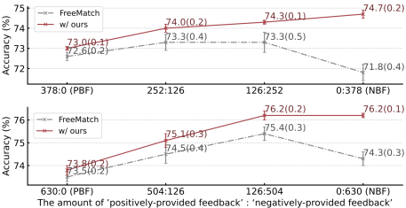
We study the role of feedback on the adaptation results by varying feedback configurations. Let positively-provided feedback (PF) be obtained from samples that the source model correctly predicts, as opposed to negatively-provided feedback (NF). We adjust the ratio of PF:NF while keeping the total number of labeled samples constant, as shown in Figure 5.
When using only FreeMatch (gray dot-dashed line), both biased feedback types (i.e., NBF and PBF) result in worse adaptation performance compared to balanced feedback for the baseline, e.g., 72.6 in 378:0 (PBF) 73.3 in 252:126. In contrast, when our method is applied (red line), NBF yields the best performance. PBF and NBF can be respectively regarded as contributing previously known knowledge of the model and new knowledge that complements model deficiencies. Hence, it may be natural that NBF, which actually encodes the model’s mistakes, contributes to favorable adaptation results.
Number of unlabeled samples in a mini-batch. Existing SemiSDA methods [6, 81] typically set the ratio between labeled and unlabeled samples in a mini-batch to 1:7. However, we observe that adhering to this ratio is not optimal for our approach, as shown in Table 7. Our method shows better performance when the ratio is varied to 1:4, i.e., decreasing unlabeled sample sizes. This finding contradicts observations in several TTA works [48, 28, 67], where adaptation performance tends to increase with larger batch sizes. We speculate that it is beneficial to prioritize more reliable information, which refers to labeled data and our defending samples selected from the filtering-applied bank, during the adapting process. This result may be aligned with previous works for curriculum learning [100, 40] and adaptive thresholding [96].
| method | feed. | negatively biased feedback (NBF) | ||
| # , # , # | 112, 0, 16 | 112, 48, 16 | 64, 48, 16 | |
| total batch size | 128 | 176 | 128 | |
| FreeMatch [81] | 72.0 | 74.2 | 74.8 (+0.6) | |
| AdaMatch [6] | 368 | 64.5 | 71.3 | 72.0 (+0.7) |
| \hdashlineFreeMatch [81] | 74.4 | 75.5 | 76.1 (+0.6) | |
| AdaMatch [6] | 630 | 67.7 | 73.4 | 74.3 (+0.9) |
Number of labeled data. We measure the impact of feedback size (number of labeled samples) in Figure 6. The results show that the inferior performance on NBF persists even with an increased amount of feedback (gray → black line); however, our approach mitigates it and improves performance (black → red line). We make an interesting observation that the performance gap between black and red lines becomes larger as the number of available feedback decreases. Since obtaining large feedback may be challenging in real-world applications, our method is expected to be more helpful in this practical case.

| selection strategy | random | random | kmeans | cosine | baseline | |
| class-aware | ✗ | ✓ | ✓ | ✓ | - | |
| FreeMatch [81] | Res. | 74.1 | 74.8 | 74.6 | 74.0 | 72.0 |
| FreeMatch [81] | ViT. | 75.0 | 75.7 | 75.6 | 75.1 | 73.9 |
| filtering rate | 0.2 | 0.4 | 0.6 | 0.8 | baseline only | |
| FreeMatch [81] | Res. | 74.5 | 74.8 | 74.3 | 73.7 | 72.0 |
| FreeMatch [81] | ViT. | 75.5 | 75.7 | 75.9 | 75.5 | 73.9 |
Data selecting strategy. We explore various strategies for selecting defending samples to balance the mini-batch, as shown in Table 8 (top). The strategies include: in the candidate bank, (i) random selection regardless of the class of the labeled data, (ii) random selection in the same class as the labeled data (i.e., class-aware), (iii) selecting samples close to the cluster center obtained by k means clustering [21] and (iv) selecting samples with embedded features distant from the labeled data where cosine distance is used. While our approach consistently outperforms the baseline regardless of the chosen strategy, we empirically find that strategy (ii) achieves the best performance. Therefore, we adopt this strategy for our proposed method.
Further studies, such as extension to a TTA scenario, combining with SFDA methods and different feedback configurations, are presented in Appendix C.
6 Conclusion & Discussion
User feedback can play an integral part in adapting the practical ML product to the target environment. However, we have shown that naive adaptation using existing SemiSDA methods led to undesirable adaptation results. We explained this through the lens of Negatively-Biased Feedback (NBF). In this paper, we uncovered the unexpected results of NBF and presented a scalable solution, Retrieval Latent Defending. This method prevents the mini-batch from becoming overly dependent on labeled samples that may have a biased distribution within the overall target distribution. Under the diverse DA benchmarks, from the simulation study to the medical imaging task, we demonstrated the practical problem caused by NBF and the effectiveness of our approach by combining it with multiple SemiSDA baselines. We hope our efforts will inspire future DA works on leveraging user feedback to improve an ML model in the deployment environment.
Broader impact. The proposed setup assumes that an ML product obtains feedback as a form of annotations (i.e., labeled data). In some cases, users can provide feedback in different forms, like thumbs up & down and rating of model prediction, or noise feedback whose information is different from the ground truth. Further research considering these points will pave the way for developing safer and more reliable adapting strategies.
Acknowledgment. We sincerely appreciate the abundant support provided by Lunit Inc., and we would like to thank Donggeun Yoo, Seonwook Park, and Sérgio Pereira for their valuable feedback.
References
- [1] Arazo, E., Ortego, D., Albert, P., O’Connor, N.E., McGuinness, K.: Pseudo-labeling and confirmation bias in deep semi-supervised learning. In: International Joint Conference on Neural Networks (IJCNN) (2020)
- [2] Basak, H., Yin, Z.: Semi-supervised domain adaptive medical image segmentation through consistency regularized disentangled contrastive learning. In: International Conference on Medical Image Computing and Computer-Assisted Intervention (2023)
- [3] Baumeister, R.F., Bratslavsky, E., Finkenauer, C., Vohs, K.D.: Bad is stronger than good. Review of general psychology (2001)
- [4] Berthelot, D., Carlini, N., Cubuk, E.D., Kurakin, A., Sohn, K., Zhang, H., Raffel, C.: Remixmatch: Semi-supervised learning with distribution alignment and augmentation anchoring. In: ICLR (2020)
- [5] Berthelot, D., Carlini, N., Goodfellow, I., Papernot, N., Oliver, A., Raffel, C.A.: Mixmatch: A holistic approach to semi-supervised learning. In: NeurIPS (2019)
- [6] Berthelot, D., Roelofs, R., Sohn, K., Carlini, N., Kurakin, A.: Adamatch: A unified approach to semi-supervised learning and domain adaptation. In: ICLR (2022)
- [7] Bradley, A.P.: The use of the area under the roc curve in the evaluation of machine learning algorithms. Pattern recognition (1997)
- [8] Chen, D., Wang, D., Darrell, T., Ebrahimi, S.: Contrastive test-time adaptation. In: CVPR (2022)
- [9] Chen, H., Tao, R., Fan, Y., Wang, Y., Wang, J., Schiele, B., Xie, X., Raj, B., Savvides, M.: Softmatch: Addressing the quantity-quality trade-off in semi-supervised learning. In: ICLR (2023)
- [10] Chen, W., Lin, L., Yang, S., Xie, D., Pu, S., Zhuang, Y.: Self-supervised noisy label learning for source-free unsupervised domain adaptation. In: IROS (2022)
- [11] Chen, X., Zhao, Z., Zhang, Y., Duan, M., Qi, D., Zhao, H.: Focalclick: Towards practical interactive image segmentation. In: CVPR (2022)
- [12] Chen, Y., Tan, X., Zhao, B., Chen, Z., Song, R., Liang, J., Lu, X.: Boosting semi-supervised learning by exploiting all unlabeled data. In: CVPR (2023)
- [13] Cohen, J.P., Viviano, J.D., Bertin, P., Morrison, P., Torabian, P., Guarrera, M., Lungren, M.P., Chaudhari, A., Brooks, R., Hashir, M., et al.: Torchxrayvision: A library of chest x-ray datasets and models. In: International Conference on Medical Imaging with Deep Learning (2022)
- [14] Cordts, M., Omran, M., Ramos, S., Rehfeld, T., Enzweiler, M., Benenson, R., Franke, U., Roth, S., Schiele, B.: The cityscapes dataset for semantic urban scene understanding. In: CVPR (2016)
- [15] Dosovitskiy, A., Beyer, L., Kolesnikov, A., Weissenborn, D., Zhai, X., Unterthiner, T., Dehghani, M., Minderer, M., Heigold, G., Gelly, S., et al.: An image is worth 16x16 words: Transformers for image recognition at scale. In: ICLR (2021)
- [16] Fini, E., Astolfi, P., Alahari, K., Alameda-Pineda, X., Mairal, J., Nabi, M., Ricci, E.: Semi-supervised learning made simple with self-supervised clustering. In: CVPR (2023)
- [17] Ganin, Y., Lempitsky, V.: Unsupervised domain adaptation by backpropagation. In: ICML (2015)
- [18] Ganin, Y., Ustinova, E., Ajakan, H., Germain, P., Larochelle, H., Laviolette, F., Marchand, M., Lempitsky, V.: Domain-adversarial training of neural networks. The journal of machine learning research (2016)
- [19] Gong, T., Jeong, J., Kim, T., Kim, Y., Shin, J., Lee, S.J.: Robust continual test-time adaptation: Instance-aware bn and prediction-balanced memory. In: NeurIPS (2023)
- [20] Harada, S., Bise, R., Araki, K., Yoshizawa, A., Terada, K., Kurata, M., Nakajima, N., Abe, H., Ushiku, T., Uchida, S.: Cluster-guided semi-supervised domain adaptation for imbalanced medical image classification. arXiv preprint arXiv:2303.01283 (2023)
- [21] Hartigan, J.A., Wong, M.A.: Algorithm as 136: A k-means clustering algorithm. Journal of the royal statistical society. series c (applied statistics) (1979)
- [22] He, K., Fan, H., Wu, Y., Xie, S., Girshick, R.: Momentum contrast for unsupervised visual representation learning. In: CVPR (2020)
- [23] He, K., Zhang, X., Ren, S., Sun, J.: Deep residual learning for image recognition. In: CVPR (2016)
- [24] Higuchi, Y., Moritz, N., Roux, J.L., Hori, T.: Momentum pseudo-labeling for semi-supervised speech recognition. In: Interspeech (2021)
- [25] Huang, D., Li, J., Chen, W., Huang, J., Chai, Z., Li, G.: Divide and adapt: Active domain adaptation via customized learning. In: CVPR (2023)
- [26] Huang, G., Liu, Z., Van Der Maaten, L., Weinberger, K.Q.: Densely connected convolutional networks. In: CVPR (2017)
- [27] Johnson, A.E., Pollard, T.J., Greenbaum, N.R., Lungren, M.P., Deng, C.y., Peng, Y., Lu, Z., Mark, R.G., Berkowitz, S.J., Horng, S.: Mimic-cxr-jpg, a large publicly available database of labeled chest radiographs. arXiv preprint arXiv:1901.07042 (2019)
- [28] Khurana, A., Paul, S., Rai, P., Biswas, S., Aggarwal, G.: Sita: Single image test-time adaptation. arXiv preprint arXiv:2112.02355 (2021)
- [29] Kim, J., Hur, Y., Park, S., Yang, E., Hwang, S.J., Shin, J.: Distribution aligning refinery of pseudo-label for imbalanced semi-supervised learning. In: NeurIPS (2020)
- [30] Knox, W.B., Stone, P.: Tamer: Training an agent manually via evaluative reinforcement. In: IEEE international conference on development and learning (2008)
- [31] Lee, H., Shin, S., Kim, H.: Abc: Auxiliary balanced classifier for class-imbalanced semi-supervised learning. In: NeurIPS (2021)
- [32] Lenga, M., Schulz, H., Saalbach, A.: Continual learning for domain adaptation in chest x-ray classification. In: Medical Imaging with Deep Learning (2020)
- [33] Li, J., Li, G., Shi, Y., Yu, Y.: Cross-domain adaptive clustering for semi-supervised domain adaptation. In: CVPR (2021)
- [34] Liang, J., Hu, D., Feng, J.: Do we really need to access the source data? source hypothesis transfer for unsupervised domain adaptation. In: ICML (2020)
- [35] Litrico, M., Del Bue, A., Morerio, P.: Guiding pseudo-labels with uncertainty estimation for source-free unsupervised domain adaptation. In: CVPR (2023)
- [36] Liu, X., Xing, F., Shusharina, N., Lim, R., Jay Kuo, C.C., El Fakhri, G., Woo, J.: Act: Semi-supervised domain-adaptive medical image segmentation with asymmetric co-training. In: International Conference on Medical Image Computing and Computer-Assisted Intervention (2022)
- [37] Liu, X., Yoo, C., Xing, F., Oh, H., El Fakhri, G., Kang, J.W., Woo, J., et al.: Deep unsupervised domain adaptation: A review of recent advances and perspectives. APSIPA Transactions on Signal and Information Processing (2022)
- [38] Liu, Y., Zhang, W., Wang, J.: Source-free domain adaptation for semantic segmentation. In: CVPR (2021)
- [39] Liu, Y., Kothari, P., van Delft, B., Bellot-Gurlet, B., Mordan, T., Alahi, A.: Ttt++: When does self-supervised test-time training fail or thrive? In: NeurIPS (2021)
- [40] Liu, Z., Miao, Z., Pan, X., Zhan, X., Lin, D., Yu, S.X., Gong, B.: Open compound domain adaptation. In: CVPR (2020)
- [41] Long, M., Zhu, H., Wang, J., Jordan, M.I.: Deep transfer learning with joint adaptation networks. In: ICML (2017)
- [42] MacGlashan, J., Ho, M.K., Loftin, R., Peng, B., Wang, G., Roberts, D.L., Taylor, M.E., Littman, M.L.: Interactive learning from policy-dependent human feedback. In: International conference on machine learning (2017)
- [43] Madani, A., Moradi, M., Karargyris, A., Syeda-Mahmood, T.: Semi-supervised learning with generative adversarial networks for chest x-ray classification with ability of data domain adaptation. In: International symposium on biomedical imaging (2018)
- [44] Mahapatra, D., Korevaar, S., Bozorgtabar, B., Tennakoon, R.: Unsupervised domain adaptation using feature disentanglement and gcns for medical image classification. In: ECCV (2022)
- [45] Mei, K., Zhu, C., Zou, J., Zhang, S.: Instance adaptive self-training for unsupervised domain adaptation. In: ECCV (2020)
- [46] Mei, K., Zhu, C., Zou, J., Zhang, S.: Instance adaptive self-training for unsupervised domain adaptation. In: ECCV (2020)
- [47] Niu, S., Wu, J., Zhang, Y., Chen, Y., Zheng, S., Zhao, P., Tan, M.: Efficient test-time model adaptation without forgetting. In: ICML (2022)
- [48] Niu, S., Wu, J., Zhang, Y., Wen, Z., Chen, Y., Zhao, P., Tan, M.: Towards stable test-time adaptation in dynamic wild world. In: ICLR (2023)
- [49] Oh, Y., Kim, D.J., Kweon, I.S.: Daso: Distribution-aware semantics-oriented pseudo-label for imbalanced semi-supervised learning. In: CVPR (2022)
- [50] Ouyang, L., Wu, J., Jiang, X., Almeida, D., Wainwright, C., Mishkin, P., Zhang, C., Agarwal, S., Slama, K., Ray, A., et al.: Training language models to follow instructions with human feedback. In: NeurIPS (2022)
- [51] Pan, Y., Yao, T., Li, Y., Wang, Y., Ngo, C.W., Mei, T.: Transferrable prototypical networks for unsupervised domain adaptation. In: CVPR (2019)
- [52] Paszke, A., Gross, S., Massa, F., Lerer, A., Bradbury, J., Chanan, G., Killeen, T., Lin, e.a.: Pytorch: An imperative style, high-performance deep learning library. In: NeurIPS (2019), https://github.com/pytorch/vision/blob/main/torchvision/models/resnet.py
- [53] Pedregosa, F., Varoquaux, G., Gramfort, A., Michel, V., Thirion, B., Grisel, O., Blondel, M., Prettenhofer, P., Weiss, R., Dubourg, V., Vanderplas, J., Passos, A., Cournapeau, D., Brucher, M., Perrot, M., Duchesnay, E.: Scikit-learn: Machine learning in Python. Journal of Machine Learning Research (2011)
- [54] Peng, X., Bai, Q., Xia, X., Huang, Z., Saenko, K., Wang, B.: Moment matching for multi-source domain adaptation. In: ICCV (2019)
- [55] Prabhu, V., Chandrasekaran, A., Saenko, K., Hoffman, J.: Active domain adaptation via clustering uncertainty-weighted embeddings. In: ICCV (2021)
- [56] Richter, S.R., Vineet, V., Roth, S., Koltun, V.: Playing for data: Ground truth from computer games. In: ECCV (2016)
- [57] Rozin, P., Royzman, E.B.: Negativity bias, negativity dominance, and contagion. Personality and social psychology review (2001)
- [58] Saito, K., Kim, D., Sclaroff, S., Darrell, T., Saenko, K.: Semi-supervised domain adaptation via minimax entropy. In: ICCV (2019)
- [59] Saito, K., Watanabe, K., Ushiku, Y., Harada, T.: Maximum classifier discrepancy for unsupervised domain adaptation. In: CVPR (2018)
- [60] Sajjadi, M., Javanmardi, M., Tasdizen, T.: Regularization with stochastic transformations and perturbations for deep semi-supervised learning. In: NeurIPS (2016)
- [61] Schulman, J., Zoph, B., Kim, C., Hilton, J., Menick, J., Weng, J., Uribe, J.F.C., Fedus, L., Metz, L., Pokorny, M., et al.: Chatgpt: Optimizing language models for dialogue. OpenAI blog (2022)
- [62] Shen, Y., Yun, H., Lipton, Z.C., Kronrod, Y., Anandkumar, A.: Deep active learning for named entity recognition. In: ICLR (2017)
- [63] Shin, I., Kim, D.J., Cho, J.W., Woo, S., Park, K., Kweon, I.S.: Labor: Labeling only if required for domain adaptive semantic segmentation. In: ICCV (2021)
- [64] Sofiiuk, K., Petrov, I., Barinova, O., Konushin, A.: f-brs: Rethinking backpropagating refinement for interactive segmentation. In: CVPR (2020)
- [65] Sofiiuk, K., Petrov, I.A., Konushin, A.: Reviving iterative training with mask guidance for interactive segmentation. In: IEEE International Conference on Image Processing (ICIP) (2022)
- [66] Sohn, K., Berthelot, D., Carlini, N., Zhang, Z., Zhang, H., Raffel, C.A., Cubuk, E.D., Kurakin, A., Li, C.L.: Fixmatch: Simplifying semi-supervised learning with consistency and confidence. In: NeurIPS (2020)
- [67] Song, J., Lee, J., Kweon, I.S., Choi, S.: Ecotta: Memory-efficient continual test-time adaptation via self-distilled regularization. In: CVPR (2023)
- [68] Song, J., Park, K., Shin, I., Woo, S., Zhang, C., Kweon, I.S.: Test-time adaptation in the dynamic world with compound domain knowledge management. IEEE Robotics and Automation Letters (2023)
- [69] Stiennon, N., Ouyang, L., Wu, J., Ziegler, D., Lowe, R., Voss, C., Radford, A., Amodei, D., Christiano, P.F.: Learning to summarize with human feedback. In: NeurIPS (2020)
- [70] Sun, B., Saenko, K.: Deep coral: Correlation alignment for deep domain adaptation. In: ECCV Workshops (2016)
- [71] Touvron, H., Martin, L., Stone, K., Albert, P., Almahairi, A., Babaei, Y., Bashlykov, N., Batra, S., Bhargava, P., Bhosale, S., et al.: Llama 2: Open foundation and fine-tuned chat models. arXiv preprint arXiv:2307.09288 (2023)
- [72] Tsai, Y.H., Hung, W.C., Schulter, S., Sohn, K., Yang, M.H., Chandraker, M.: Learning to adapt structured output space for semantic segmentation. In: CVPR (2018)
- [73] Tsai, Y.H., Hung, W.C., Schulter, S., Sohn, K., Yang, M.H., Chandraker, M.: Learning to adapt structured output space for semantic segmentation. In: CVPR (2018)
- [74] Van Engelen, J.E., Hoos, H.H.: A survey on semi-supervised learning. Machine learning (2020)
- [75] Venkateswara, H., Eusebio, J., Chakraborty, S., Panchanathan, S.: Deep hashing network for unsupervised domain adaptation. In: CVPR (2017)
- [76] Vu, T.H., Jain, H., Bucher, M., Cord, M., Pérez, P.: Advent: Adversarial entropy minimization for domain adaptation in semantic segmentation. In: CVPR (2019)
- [77] Wang, D., Shelhamer, E., Liu, S., Olshausen, B., Darrell, T.: Tent: Fully test-time adaptation by entropy minimization. In: ICLR (2021)
- [78] Wang, M., Deng, W.: Deep visual domain adaptation: A survey. Neurocomputing (2018)
- [79] Wang, Q., Fink, O., Van Gool, L., Dai, D.: Continual test-time domain adaptation. In: CVPR (2022)
- [80] Wang, Y., Chen, H., Fan, Y., Sun, W., Tao, R., Hou, W., Wang, R., Yang, L., Zhou, Z., Guo, L.Z., et al.: Usb: A unified semi-supervised learning benchmark for classification. In: NeurIPS (2022)
- [81] Wang, Y., Chen, H., Heng, Q., Hou, W., Fan, Y., Wu, Z., Wang, J., Savvides, M., Shinozaki, T., Raj, B., et al.: Freematch: Self-adaptive thresholding for semi-supervised learning. In: ICLR (2023)
- [82] Warnell, G., Waytowich, N., Lawhern, V., Stone, P.: Deep tamer: Interactive agent shaping in high-dimensional state spaces. In: AAAI (2018)
- [83] Wei, C., Sohn, K., Mellina, C., Yuille, A., Yang, F.: Crest: A class-rebalancing self-training framework for imbalanced semi-supervised learning. In: CVPR (2021)
- [84] Wirth, C., Akrour, R., Neumann, G., Fürnkranz, J., et al.: A survey of preference-based reinforcement learning methods. Journal of Machine Learning Research (2017)
- [85] Xie, B., Yuan, L., Li, S., Liu, C.H., Cheng, X.: Towards fewer annotations: Active learning via region impurity and prediction uncertainty for domain adaptive semantic segmentation. In: CVPR (2022)
- [86] Xie, M., Li, Y., Wang, Y., Luo, Z., Gan, Z., Sun, Z., Chi, M., Wang, C., Wang, P.: Learning distinctive margin toward active domain adaptation. In: CVPR (2022)
- [87] Xie, Q., Dai, Z., Hovy, E., Luong, T., Le, Q.: Unsupervised data augmentation for consistency training. In: NeurIPS (2020)
- [88] Xu, Y., Shang, L., Ye, J., Qian, Q., Li, Y.F., Sun, B., Li, H., Jin, R.: Dash: Semi-supervised learning with dynamic thresholding. In: ICML (2021)
- [89] Yan, Z., Wu, Y., Li, G., Qin, Y., Han, X., Cui, S.: Multi-level consistency learning for semi-supervised domain adaptation. In: IJCAI (2022)
- [90] Yang, L., Wang, Y., Gao, M., Shrivastava, A., Weinberger, K.Q., Chao, W.L., Lim, S.N.: Deep co-training with task decomposition for semi-supervised domain adaptation. In: ICCV (2021)
- [91] Yang, S., Jui, S., van de Weijer, J., et al.: Attracting and dispersing: A simple approach for source-free domain adaptation. In: NeurIPS (2022)
- [92] Yang, S., Wang, Y., Van De Weijer, J., Herranz, L., Jui, S.: Generalized source-free domain adaptation. In: ICCV (2021)
- [93] Yang, S., van de Weijer, J., Herranz, L., Jui, S., et al.: Exploiting the intrinsic neighborhood structure for source-free domain adaptation. In: NeurIPS (2021)
- [94] Yu, Y.C., Lin, H.T.: Semi-supervised domain adaptation with source label adaptation. In: CVPR (2023)
- [95] Yu, Z., Li, J., Du, Z., Zhu, L., Shen, H.T.: A comprehensive survey on source-free domain adaptation. arXiv preprint arXiv:2302.11803 (2023)
- [96] Zhang, B., Wang, Y., Hou, W., Wu, H., Wang, J., Okumura, M., Shinozaki, T.: Flexmatch: Boosting semi-supervised learning with curriculum pseudo labeling. In: NeurIPS (2021)
- [97] Zhang, C., Miech, A., Shen, J., Alayrac, J.B., Luc, P.: Making the most of what you have: Adapting pre-trained visual language models in the low-data regime. arXiv preprint arXiv:2305.02297 (2023)
- [98] Zhang, W., Ouyang, W., Li, W., Xu, D.: Collaborative and adversarial network for unsupervised domain adaptation. In: CVPR (2018)
- [99] Zhang, Y., Zhang, H., Deng, B., Li, S., Jia, K., Zhang, L.: Semi-supervised models are strong unsupervised domain adaptation learners. arXiv preprint arXiv:2106.00417 (2021)
- [100] Zhang, Y., David, P., Gong, B.: Curriculum domain adaptation for semantic segmentation of urban scenes. In: ICCV (2017)
- [101] Zhang, Y., Wang, Z., He, W.: Class relationship embedded learning for source-free unsupervised domain adaptation. In: CVPR (2023)
Supplementary Material on Is user feedback always informative? Retrieval Latent Defending for Semi-Supervised Domain Adaptation without Source Data
Junha Song Tae Soo Kim Junha Kim Gunhee Nam Thijs Kooi Jaegul Choo
In this supplementary material, we provide:
A Comparison with Related Work
A.1 Active Domain Adaptation
Active domain adaptation (ActiveDA) aims to select the most informative samples being labeled by annotators, given a limited annotating budget. As shown in Figure 7, the machine selects some samples using ActiveDA methods and instructs annotators to label the selected samples. Several ActiveDA methods have been proposed, such as CLUE [55], which employs an entropy-based clustering algorithm to preserve the uncertainty and diversity of labeled data. SDM-AG [86] and DiaNa [25] utilize margin functions between the source and target domains to identify informative samples. In contrast to this ActiveDA scenario, we present an NBF scenario where there is no machine-instructed sample selection, and instead, users directly provide feedback as a response to the prediction result. It may lead to more flexible applications since (1) users have the freedom to choose samples, and (2) individual users can impose different standards in selecting samples.

We note that ActiveDA methods are for of Figure 7, while our method is for and proposed to alleviate the problem caused by NBF. Although out of our scope, we evaluate our method under ActiveDA labeling scenarios, where CLUE and DiaNA1 are employed. The results in Table 9 suggest two points. First, our method complements existing ActiveDA methods, consistently improving their performance. This highlights the importance of adapting the model with a balanced supervised signal throughout adaptation (i.e., stage C) using our method, even when ActiveDA methods like CLUE respect the diversity of labeled samples. Second, our method achieves significant performance gains regardless of the labeling scenario, showing that our method can be applied for reliable adaptation even when the distribution of labeled data is unknown.
| state B | |||||||
| feed. amount | 378 (3 labeled data per class) | 1890 | 5040 | ||||
| stage C | RF | NBF | Entropy [62] | CLUE [55] | DiaNA [25] | CLUE [55] | CLUE [55] |
| AdaMatch [7] | 67.6 | 64.5 | 65.9 | 68.6 | 68.1 | 76.1 | 80.3 |
| w/ ours | 71.1 (+3.5) | 72.0 (+7.5) | 71.1 (+5.2) | 71.5 (+2.9) | 71.3 (+3.2) | 78.0 (+1.9) | 81.4 (+1.1) |
A.2 Class-Imbalanced Semi-Supervised Learning
SemiSDA and SemiSL methods often struggle with the different numbers of labeled data between classes, known as class imbalance [49]. To address this problem, class-imbalanced SemiSL works like CReST [83] propose to balance the quantity of labeled data by using pseudo labels [29, 31] in stage D (i.e., generation in CReST) of Figure 7. Recent advancements like DASO [49] further reduce the imbalance effect using both a similarity-based and linear classifier. Despite such advances in class-imbalanced SemiSL, the biased (i.e., imbalanced) label distribution within the same class has been overlooked in the SemiSDA, SemiSL, and class-imbalanced SemiSL works. Therefore, we introduce the new concept of biased labeled data called NBF and demonstrate its unexpected influence on adaptation performance.
Even though our focus in this paper is on the bias within the same class, accounting for the imbalance between classes can still be crucial for reliable domain adaptation. For example, in the medical domain, while radiologists are likely to log the mistakes of the model, the amount of feedback from false negative samples may be small compared to those from false positive samples, given the natural prevalence of disease (e.g., lung cancer is less than 1 in 1000). We simulate this example scenario and evaluate our method in Table 10.
| method | feedback | FP : FN | average | fracture | pneumothorax | |
| Source model | - | - | .6768 | .6642 | .6894 | |
| Pseudo-Label. [1] | RF | - | .7325 | .7541 | .7109 | |
| \hdashline | NBF | 40 : 40 | .7173 (-.0152) | .7414 (-.0127) | .6931 (-.0178) | |
| with ours | NBF | 40 : 40 | .7334(+.0162) | .7625 (+.0211) | .7044 (+.0113) | |
| \cdashline2-7 | NBF | 75 : 5 | .7248 (-.0077) | .7494 (-.0047) | .7002 (-.0107) | |
| with ours | NBF | 75 : 5 | .7361 (+.0113) | .7653 (+.0159) | .7070 (+.0068) | |
| \cdashline2-7 | NBF | 5 : 75 | .7170 (-.0155) | .7420 (-.0121) | .6921 (-.0188) | |
| 80 feedback | with ours | NBF | 5 : 75 | .7315 (+.0145) | .7679 (+.0260) | .6951 (+.0030) |
| Pseudo-Label. [1] | RF | - | .7353 | .7565 | .7141 | |
| \hdashline | NBF | 80 : 80 | .7162 (-.0192) | .7429 (-.0136) | ..6894 (-.0247) | |
| with ours | NBF | 80 : 80 | .7331 (+.0169) | .7680 (+.0251) | .6983 (+.0088) | |
| \cdashline2-7 | NBF | 155 : 5 | .7237 (-.0117) | .7559 (-.0007) | .6915 (-.0227) | |
| with ours | NBF | 155 : 5 | .7358 (+.0121) | .7665 (+.0106) | .7051 (+.0136) | |
| \cdashline2-7 | NBF | 5 : 155 | .7166 (-.0188) | .7438 (-.0128) | .6894 (-.0248) | |
| 160 feedback | with ours | NBF | 5 : 155 | .7300 (+.0134) | .7696 (+.0258) | .6904 (+.0010) |
| Fully supervised | - | - | .7744 | .8003 | .7486 |
Under different feedback configurations.
We take various feedback configurations into account, as depicted in Table 10. Assuming the model acquires 80 or 160 feedback instances for each finding, we alter the feedback quantities from false positive (FP) and false negative (FN) errors, which is similar to the setup of class-imbalanced SemiSL [83, 29]. We only consider two radiographic findings for simplification. The results show that our method can also mitigate the intended impact of NBF even with the class-imbalanced scenario. Interestingly, we observe better performance when FP feedback is larger than FN feedback, which makes our method suitable for the medical domain, where radiographic findings are rarely detected due to the natural prevalence of the disease.
Combining with class-imbalanced SemiSL methods.
One naive way to more reliably adapt to the challenging scenario could involve combining our method with class-imbalanced SemiSL methods in stages C and D of Figure 7. To evaluate this approach, we conduct an additional simulation study in Figure 8. The simulation replicates the NBF scenario by selecting only misclassified samples within the same class. We further introduce class imbalance by varying the number of feedback points between the blue and orange classes (leftmost sub-figure).
By adapting the model with different approaches, we can find two interesting takeaways: (1) the approach proposed in CReST [83] was not designed to solve the unexpected effect of NBF, so it struggles with adaptation under the challenging scenario. (2) our method achieves better adaptation performance than using only CReST, and outperforms other results by combining with CReST. These results highlight the importance of considering an NBF case as well as a class-imbalance problem and the efficiency of our method. We hypothesize that defending the latent class space throughout adapting iterations helps the model to be robust to the effect of NBF, different from a previous generation-based approach in CReST [83]. In addition, a discussion about zero feedback for certain classes is provided in Section C.

A.3 Test-time Adaptation
To mitigate performance degradation caused by domain shift, models deployed on edge devices like smartphones and self-driving cars can be adapted to the target domain in an online manner, referred to as test-time adaptation (TTA). TTA assumes two practical settings: i) adapting without source data and ii) storing a limited amount of unlabeled target data. For instance, TENT [77, 47, 67, 68] leverages the current batch of unlabeled data to update the model’s batch normalization parameters. Alternatively, methods like NOTE [19] and ContraTTA [8] employ a target memory bank where a small amount of data (e.g., 16k image features in ContraTTA) can be only stored and used for adaptation.
Extension to a TTA scenario.
Our setup illustrated in Figure 2 also assumes a source-free setup, so it can be easily extended to a TTA scenario by employing the memory bank. In particular, on a periodic basis, when 10% of the target training data is encountered, an adaptation is executed following a TTA setup of TTT++ [39] and ContraTTA [8], where unlabeled data in the memory bank and labeled data are utilized. The memory bank size is set to 5k pseudo labels, and FreeMatch [81] is used for a SemiSDA baseline algorithm. It should be noted that since previous TTA works do not consider the utilization of labeled data, we can not use them as a baseline or compare the adaptation performance directly (but we attempt to alleviate this problem and implement comparisons in Section C.). The results in Table 11 show that our method works well even with a smaller amount of unlabeled data in the memory bank. We find this result very surprising and wish to continue in this direction for future research.
| memory bank size = 5k | percentage of target data encountered in target domain | |||||
|---|---|---|---|---|---|---|
| method | feed. | amo. | 10% 40% 70% 100% | |||
| FreeMatch [81] | RF | 68.4 | 71.4 | 73.0 | 73.4 | |
| NBF | 66.9 | 69.5 | 71.0 | 71.5 | ||
| w/ ours | NBF | 368 | 68.9 (+2.0) | 72.4 (+2.9) | 73.6 (+2.6) | 74.3 (+2.8) |
| FreeMatch [81] | RF | 71.2 | 73.7 | 74.7 | 75.4 | |
| NBF | 69.8 | 72.2 | 73.2 | 73.9 | ||
| w/ ours | NBF | 630 | 71.5 (+1.7) | 74.1 (+1.9) | 75.0 (+1.8) | 75.5 (+1.6) |
A.4 Learning with User Feedback
Learning with User Feedback has garnered significant attention for its effectiveness in capturing users’ preferences or intentions [84, 69, 42, 50]. Reinforcement learning from human feedback is a powerful technique for model optimization based on human-provided rewards [30, 82, 61, 71]. Another application is interactive image segmentation [65, 64, 11], where users provide pixel-level annotations, enabling the model to enhance its understanding of user preferences over time.
B Further understanding with Simulation Study
In this section, we provide additional details and understanding about the simulation study in Figure 3.
Network architecture.
We build the model consisting of three fully connected layers and Relu activation functions. This model takes the point coordinate as input and returns the class label as output. Please refer to example codes found in the ‘sklearn.datasets.make_blobs’ documents [53].
Baseline.
One simple SemiSL method, Pseudo labeling [1], can be easily applied to the toy experiment. Given a mini-batch with labeled data and unlabeled data , we simply adapt the model with cross-entropy losses as the following:
|
|
(3) |
is the output probability from the model and refers to the pseudo label. As shown in the equation, the updating model continuously predicts pseudo labels for the unlabeled data. So, the pseudo labels can be changed based on an updated decision boundary. Figure 9 presents this phenomenon as the adapting epoch progresses.
Additional study on two moon dataset.
To better understand the unexpected influence of NBF on domain adaptation, we conducted additional simulations using the two moon datasets from scikit-learn [53]. As shown in Figure 10, we generate source and target data so that they have domain shifts. After pre-training a model on the source data, we evaluate its performance on the target domain, observing a performance drop due to the shift (99.9%→81.4%). After we simulate user-provided feedback under two scenarios (i.e., RF and NBF), we adapt the model to the target data in a semi-supervised manner [1]. The results highlight crucial observations shown in Section 3.2: the distribution of label data significantly impacts adaptation performance. Notably, biased feedback distribution (NBF) leads to poorer performance compared to evenly distributed feedback (RF). In our main paper, we showed that this problem remained the same even with state-of-the-art SemiSDA methods and under different DA benchmarks.


C Additional Ablation Study
Reliable sample filtering.
An important design of our approach is to retain only samples having reliable pseudo labels among . We evaluate the adaptation performance with variations in the filtering ratio in Table 8. A higher increases the likelihood of the bank being contaminated with samples with incorrect pseudo labels (i.e., ) while a lower decreases the diversity of the defending samples. We observe that our approach is robust to the hyper-parameter , yet achieves reasonable performance with .
Combining with SFDA methods.
Recent SFDA methods [34, 35] have shown promise in computing the unsupervised loss . So, we explore their potential as baselines within our framework. To construct the overall loss function in Eq. (2), we simply combine their with the supervised loss of FreeMatch [81] since SFDA methods do not take the utilization of supervised loss into account. The results are presented in Table 12. Interestingly, some SFDA works [34, 8, 35] using sophisticated methods, such as k-means clustering [21] and contrastive learning [22], are likely to be less susceptible to NBF. However, the trend is not consistent for all methods. NRC [93], using a strategy of nearest neighbors, shows sub-optimal performance under an NBF assumption. Notably, all SFDA methods achieve their best adaptation performance when combined with our method. This suggests that even methods that partially mitigate NBF’s unexpected effects can further benefit from our method.
| feed. amount | 378 (3 labeled data per class) | 630 (5 labeled data per class) | |||||
|---|---|---|---|---|---|---|---|
| method | RF | NBF | w/ ours | RF | NBF | w/ ours | |
| SHOT [34] | 69.6 | 70.7 (+1.1) | 71.5 (+0.8) | 71.1 | 72.3 (+1.2) | 73.0 (+0.7) | |
| NRC [93] | 66.3 | 64.9 (-1.4) | 69.3 (+4.4) | 68.5 | 66.4 (-2.1) | 69.6 (+3.2) | |
| ContraTTA [8] | 68.6 | 69.2 (+0.6) | 71.6 (+2.4) | 70.1 | 70.5 (+0.4) | 72.4 (+1.9) | |
| ResNet-50 | GuidingSP [35] | 69.7 | 70.2 (+0.5) | 71.8 (+1.6) | 70.5 | 71.0 (+0.5) | 72.8 (+1.8) |
| SHOT [34] | 73.4 | 73.7 (+0.3) | 74.1 (+0.4) | 74.4 | 74.8 (+0.4) | 75.4 (+0.6) | |
| NRC [93] | 72.2 | 71.9 (-0.3) | 72.9 (+1.0) | 73.9 | 73.7 (-0.2) | 74.6 (+0.9) | |
| ContraTTA [8] | 72.8 | 73.4 (+0.6) | 74.9 (+1.5) | 73.9 | 74.8 (+0.9) | 76.4 (+1.6) | |
| ViT-S | GuidingSP [35] | 73.3 | 73.7 (+0.4) | 75.0 (+1.3) | 74.1 | 74.9 (+0.8) | 76.4 (+1.5) |
Number of appended defending samples.
As mentioned in Section 4.2, we incorporate defending samples for each labeled data point to decrease the unexpected impact of NBF on the supervised signal. To understand how the value of affects performance, we conducted an ablation study in Table 13. We fix the number of labeled data points to 16 and maintain the total batch size at 128 by adjusting the ratio in Eq. (1). For instance, with , the ratio is set to 3 (i.e., ). Our experiments across two different architectures reveal that a value generally yields good adaptation performance. Consequently, we adopt for all experiments.
| only | the overall loss in Eq. (LABEL:2) | ||||
|---|---|---|---|---|---|
| pseudo-feedback per class | 0 | 3 | w/ ours | 5 | w/ ours |
| NRC [93] | 63.5 | 63.4 | 64.6 (+1.2) | 63.4 | 64.4 (+1.0) |
| ContrastiveTTA [8] | 66.6 | 66.6 | 67.4 (+0.8) | 66.5 | 67.2 (+0.7) |
Under a zero feedback scenario.
We note that, as previous SemiSDA [58, 6] and SemiSL [66, 81] works, we assume that a user provides a small amount of feedback (i.e., labeled data) during their interaction with an ML application. Nevertheless, we wondered about a broader question: how can our method be used when no feedback is received? This scenario, while beyond the scope of our work, presents an intriguing area for further exploration, so we attempt to investigate the potential impact of our method under such a scenario. We initially opted to use SFDA baselines of Table 12, which have demonstrated potential in the absence of labeled target data, and assess their performance within an SFDA setup (i.e., only in Table 14). Then, pseudo-feedback is generated by randomly selecting small unlabeled data sets and their pseudo-labels from samples with high predicted probabilities. With the pseudo-feedback and unlabeled target data, we conduct SemiSDA and report the results (i.e., the overall loss in Table 14). We find that i) simulating pseudo-feedback has a minor influence on SFDA baselines, yet ii) the adaptation performance is enhanced by combining with our method. Based on these results, we believe that even in the absence of feedback for certain classes, SemiSDA with our method can achieve good adaptation performance by leveraging the pseudo-feedback.
D Additional Experimental Details
Details for medical experiments.
We use DenseNet-121 [26] provided by the TorchXRayVision repository [13]. This architecture consists of a shared backbone and multiple classification heads for radiographic findings. When given a 256x256 image as input, it generates sigmoid values for thirteen different findings.
The majority of SemiSDA methods, such as AdaMatch [6] and FreeMatch [81], depend on consistency regularization, which requires image augmentation strategies, such as ColorJitter and GaussianBlur [52]. Unfortunately, applying them to medical images remains challenging, as most strategies have been proposed specifically for natural images. As a result, we employ Pseudo-labeling [1], a fundamental SemiSL algorithm that (i) obviates the necessity for image augmentations and (ii) can be easily implemented for a multi-finding binary classification setup. To be more specific, we substitute the cross-entropy in Eq. (3) with the binary cross-entropy loss. To generate pseudo labels (i.e., presence or absence in Table 5 (top)), thresholds that are pre-calculated in the source domain are used. The hyper-parameters for model updates are the following.
| batch size | learning rate | optimizer | weight decay | |
|---|---|---|---|---|
| pre-training | 128 | 1e-3 | Adam | 1e-5 |
| adaptation | 128 | 1e-4 | Adam | 1e-5 |
Details for semantic segmentation experiments.
Our experiment leverages the GTA5 [56] and Cityscapes [14] datasets as the source and target domains. To compute the supervised and unsupervised losses in Eq. (1), we employ baseline algorithms: IAST [46] in LabOR [63] and RIPU [85]. Following previous works [63, 85], we utilize ResNet-101 as the backbone architecture and DeepLab-v2 as the segmentation model. Further details regarding implementation and hyper-parameter for adaptation can be found in the publicly available codebase of RIPU [85]. One of our method’s key strengths is its simplicity, which makes it readily applicable to various tasks like semantic segmentation. To be more specific, we first identify pixel points in an image that have the top 40% probabilities for each class. Among them, we select three pixels (i.e., defending pixels) for each labeled pixel in order to balance the supervised signal (i.e., in Eq. (2)) and obtain robust adaptation performance to the unexpected effect of NBF.
E Additional Discussion
33footnotetext: We evaluate SSNL using the same experimental setup in Table 12.E.1 Technique novelty
Compared to previous works, our approach, retrieval latent defending, distinguishes itself in how balancing is applied to solve the novel NBF problem.: (i) We initially anticipated that conventional tricks using confident pseudo labels or balancing strategy, such as CReST [83] for class-imbalance, CLUE [55], DiaNA [25] for ActiveDA, GuidSP [35] and SSNLL [10] for noisy pseudo labels, would ameliorate the NBF issue. However, as shown in the table below E, we found these methods to fall short due to their lack of specific targeting of the novel problem by NBF, thereby underscoring the need for our tailored approach. (ii) Our strategy diverges from the dataset-level balancing approaches in [83, 55, 10]. Instead, we focus on enhancing the supervised signal within a minibatch through iterative retrieval of defending samples, which helps in fortifying latent spaces against the unexpected issue by NBF as illustrated in Figure 4 and Table 5. Surprisingly, this distinct method not only effectively addresses the NBF problem but also leads to substantial improvements in adaptation performance.
E.2 Computational overhead
Our method incurs only negligible overhead, as the only additional data† that needs to be stored are pseudo labels. As shown in the following table E.1, our method results in an additional 0.1 MB of memory and a 3% increase in running time compared to existing SemiSDA [6, 81] and SFDA [35] methods, but these modest increases facilitate significant performance enhancements. We adhere to the standard practices of SemiSDA and SFDA, which involve storing target images in a database (DB)‡.
| method | AdaMatch (ICLR22) | w/ ours | GuidSP (CVPR23) | w/ ours | FreeMatch (ICLR23) | w/ ours |
|---|---|---|---|---|---|---|
| reference | Table 3 | Table 3 | Table 12 | Table 12 | Table 11 | Table 11 |
| DB size‡ | 55k images | 55k images | 55k images | 55k images | 5k images | 5k images |
| add. data† | 0 MB | 0.1 MB | 53.8 MB | 53.9 MB | 0 MB | 0.01 MB |
| run. time | 132 min | 136 min | 150 min | 155 min | 14 min | 15 min |
| accuracy | 64.5 | 72.0 (+7.5) | 70.2 | 71.8 (+1.6) | 66.9 | 68.9 (+2.0) |
E.3 Limitations.
Machine learning (ML) powered products can collect target data in various ways. Beyond unlabeled data encountered in the target environment (e.g., driving scenes from a self-driving car), feedback containing valuable target information can be collected by users. For example, a radiologist can log misdiagnosed chest X-ray images in the medical application. However, leveraging effectively such feedback to enhance the deployed model has yet to be well studied. So, this paper addressed this issue by proposing a framework, domain adaptation with user feedback, as illustrated in Figure 2. Moreover, we identified potential issues (i.e., the unexpected impact of NBF) and introduced a simple and scalable solution (i.e., retrieval latent defending).
However, a few more considerations need to be made before this framework is applied in the real world. (1) Current SemiSDA and SemiSL works typically conduct a single adaptation round using all target training data. In practice, however, periodic adaptation may be required since the model can continuously collect new data. According to CoTTA [79], EATA [47], and EcoTTA [67], studies to make initial TTA research [77, 39, 8] more realistic, long-term adaptation can lead to catastrophic forgetting and error accumulation. They attempt to address this problem by utilizing continual learning strategies, e.g., random parameter restoration and knowledge distillation. Repeated adaptation processes in our setup might result in similar issues, suggesting a potential connection to continual learning techniques within the SemiSDA methods. (2) More SemiSDA methods specializing in medical imaging still need to be developed. We employed the native SemiSDA method, Pseudo-Labeling [1], in Table 5. Developing SemiSDA methods specific to medical imaging has the potential to significantly improve adaptation performance beyond the results of Table 5. It is also a promising direction for future research.
F Results of all domain shifts
In addition to Table 3, Table 5.1, and Table 12, we report the adaptation results for all domain shift scenarios in Table 15, Table 16, Table 17, Table 18, Table 19, and Table 20.
| method | feedback | average | real→clip. | real→pain. | pain.→clip. | clip.→scat. | scat.→pain. | real→scat. | pain.→real | |
|---|---|---|---|---|---|---|---|---|---|---|
| Source model | - | 56.5 | 56.1 | 63.7 | 55.2 | 48.0 | 51.7 | 45.8 | 74.7 | |
| \cdashline2-11 | FixMatch [66] | RF | 67.6 | 66.2 | 68.3 | 68.2 | 61.0 | 69.8 | 58.7 | 80.8 |
| NBF | 63.4 | 62.4 | 65.1 | 64.8 | 55.8 | 64.6 | 52.7 | 78.4 | ||
| w/ ours | NBF | 73.2 | 75.0 | 74.3 | 74.7 | 66.9 | 71.8 | 65.4 | 84.1 | |
| UDA [87] | RF | 69.2 | 68.7 | 70.0 | 69.8 | 62.8 | 70.9 | 60.0 | 82.0 | |
| NBF | 64.9 | 64.5 | 66.0 | 67.3 | 57.2 | 66.3 | 53.8 | 79.5 | ||
| w/ ours | NBF | 73.4 | 76.2 | 74.0 | 74.7 | 67.4 | 71.9 | 65.7 | 84.1 | |
| FlexMatch [96] | RF | 73.3 | 76.7 | 74.0 | 75.6 | 66.9 | 73.2 | 64.4 | 82.5 | |
| NBF | 71.4 | 74.8 | 72.2 | 74.5 | 63.8 | 71.1 | 61.7 | 81.4 | ||
| w/ ours | NBF | 74.7 | 77.9 | 74.8 | 77.8 | 68.9 | 72.2 | 66.9 | 84.4 | |
| FreeMatch [81] | RF | 73.8 | 76.6 | 74.2 | 75.5 | 67.7 | 73.5 | 65.1 | 84.0 | |
| NBF | 72.0 | 75.5 | 72.9 | 74.6 | 65.0 | 72.3 | 62.0 | 81.7 | ||
| w/ ours | NBF | 74.8 | 78.1 | 74.5 | 77.1 | 68.8 | 72.4 | 67.3 | 85.0 | |
| \cdashline2-11 | MME [58] | RF | 69.5 | 70.0 | 71.2 | 69.3 | 63.5 | 69.6 | 61.7 | 81.5 |
| NBF | 68.4 | 69.5 | 70.7 | 69.1 | 61.5 | 69.0 | 58.8 | 80.2 | ||
| w/ ours | NBF | 70.8 | 72.9 | 71.6 | 72.9 | 64.0 | 68.4 | 62.1 | 83.5 | |
| CDAC [33] | RF | 68.3 | 67.1 | 69.0 | 68.9 | 62.6 | 69.9 | 59.5 | 81.1 | |
| NBF | 64.6 | 64.5 | 66.2 | 66.3 | 56.9 | 65.8 | 53.6 | 78.6 | ||
| w/ ours | NBF | 73.2 | 76.1 | 73.9 | 74.4 | 67.0 | 71.2 | 65.8 | 84.1 | |
| AdaMatch [6] | RF | 67.6 | 66.6 | 68.5 | 68.5 | 60.3 | 69.2 | 58.7 | 81.5 | |
| NBF | 64.5 | 64.3 | 66.1 | 65.6 | 56.9 | 65.6 | 54.2 | 78.9 | ||
| ResNet-50 [23] | w/ ours | NBF | 72.0 | 74.5 | 72.7 | 73.9 | 65.5 | 70.0 | 64.3 | 83.2 |
| \cdashline2-11 | Fully sup. | - | 83.6 | 85.6 | 81.4 | 85.6 | 80.4 | 81.4 | 80.4 | 90.1 |
| Source model | - | 64.5 | 63.6 | 70.2 | 61.6 | 56.7 | 65.5 | 53.5 | 80.5 | |
| \cdashline2-11 | FixMatch [66] | RF | 74.6 | 75.5 | 77.1 | 73.8 | 67.7 | 75.9 | 67.1 | 85.1 |
| NBF | 73.0 | 73.8 | 75.4 | 74.0 | 65.1 | 72.8 | 66.1 | 83.8 | ||
| w/ ours | NBF | 75.6 | 77.1 | 77.7 | 77.3 | 67.8 | 76.8 | 68.0 | 84.7 | |
| UDA [87] | RF | 74.8 | 75.5 | 77.1 | 74.0 | 67.9 | 76.1 | 67.4 | 85.4 | |
| NBF | 73.3 | 74.1 | 75.6 | 74.3 | 65.4 | 73.2 | 66.3 | 83.9 | ||
| w/ ours | NBF | 75.8 | 77.1 | 77.8 | 77.6 | 68.2 | 77.1 | 68.2 | 84.9 | |
| FlexMatch [96] | RF | 74.9 | 75.5 | 77.0 | 74.7 | 68.4 | 76.2 | 66.7 | 85.7 | |
| NBF | 73.9 | 74.5 | 76.6 | 75.1 | 66.1 | 74.5 | 66.4 | 84.1 | ||
| w/ ours | NBF | 75.8 | 77.2 | 77.5 | 77.9 | 68.3 | 77.0 | 67.9 | 85.0 | |
| FreeMatch [81] | RF | 74.9 | 75.3 | 76.8 | 74.5 | 68.1 | 76.5 | 67.0 | 86.0 | |
| NBF | 73.9 | 74.6 | 76.4 | 75.0 | 66.0 | 74.5 | 66.5 | 84.1 | ||
| w/ ours | NBF | 75.7 | 76.9 | 77.5 | 77.9 | 68.1 | 76.7 | 67.8 | 85.2 | |
| \cdashline2-11 | MME [58] | RF | 73.2 | 74.0 | 74.8 | 73.0 | 66.5 | 74.6 | 65.2 | 84.3 |
| NBF | 72.7 | 73.2 | 74.8 | 73.8 | 65.3 | 73.0 | 64.8 | 83.8 | ||
| w/ ours | NBF | 74.1 | 75.4 | 75.9 | 76.2 | 66.2 | 74.7 | 66.4 | 84.2 | |
| CDAC [33] | RF | 74.2 | 74.8 | 76.3 | 73.8 | 67.5 | 75.5 | 66.6 | 84.9 | |
| NBF | 72.8 | 73.6 | 74.9 | 73.9 | 65.0 | 72.8 | 65.4 | 83.8 | ||
| w/ ours | NBF | 75.4 | 76.7 | 77.6 | 77.2 | 67.6 | 76.2 | 67.9 | 84.6 | |
| AdaMatch [6] | RF | 74.7 | 75.3 | 76.9 | 73.8 | 68.0 | 76.3 | 67.1 | 85.5 | |
| NBF | 73.7 | 74.7 | 76.2 | 74.7 | 65.7 | 74.0 | 66.8 | 84.0 | ||
| ViT-S [15] | w/ ours | NBF | 75.9 | 76.9 | 77.8 | 77.8 | 68.5 | 76.6 | 68.3 | 85.1 |
| \cdashline2-11 | Fully sup. | - | 85.4 | 87.8 | 83.4 | 87.8 | 81.3 | 83.4 | 81.3 | 92.7 |
| method | feedback | average | real→clip. | real→pain. | pain.→clip. | clip.→scat. | scat.→pain. | real→scat. | pain.→real | |
|---|---|---|---|---|---|---|---|---|---|---|
| Source model | - | 56.5 | 56.1 | 63.7 | 55.2 | 48.0 | 51.7 | 45.8 | 74.7 | |
| \cdashline2-11 | FixMatch [66] | RF | 71.5 | 71.3 | 70.9 | 73.1 | 65.5 | 71.9 | 65.1 | 83.0 |
| NBF | 66.1 | 66.2 | 67.6 | 67.6 | 57.4 | 67.4 | 56.5 | 79.8 | ||
| w/ ours | NBF | 75.1 | 77.2 | 75.7 | 77.2 | 69.8 | 73.9 | 68.0 | 84.1 | |
| UDA [87] | RF | 72.9 | 73.4 | 72.6 | 74.6 | 67.1 | 73.1 | 65.9 | 83.4 | |
| NBF | 68.8 | 70.3 | 68.7 | 71.1 | 60.3 | 70.3 | 60.5 | 80.5 | ||
| w/ ours | NBF | 75.3 | 78.3 | 75.2 | 77.9 | 69.6 | 73.9 | 68.1 | 84.3 | |
| FlexMatch [96] | RF | 75.3 | 78.5 | 74.6 | 77.5 | 70.3 | 73.8 | 68.7 | 83.8 | |
| NBF | 73.9 | 77.3 | 74.0 | 76.3 | 66.2 | 73.8 | 67.2 | 82.6 | ||
| w/ ours | NBF | 76.0 | 79.5 | 75.6 | 78.7 | 70.2 | 74.3 | 69.0 | 84.7 | |
| FreeMatch [81] | RF | 75.6 | 78.6 | 74.9 | 77.6 | 70.2 | 74.3 | 69.0 | 84.7 | |
| NBF | 74.4 | 77.6 | 74.5 | 76.3 | 66.8 | 73.8 | 68.2 | 83.5 | ||
| w/ ours | NBF | 76.1 | 79.6 | 75.5 | 78.6 | 70.4 | 74.5 | 69.3 | 84.9 | |
| \cdashline2-11 | MME [58] | RF | 71.2 | 71.3 | 72.1 | 71.8 | 65.6 | 70.7 | 64.6 | 82.6 |
| NBF | 70.1 | 71.4 | 71.4 | 70.4 | 62.1 | 70.7 | 62.7 | 81.8 | ||
| w/ ours | NBF | 72.5 | 74.5 | 72.7 | 74.9 | 66.4 | 70.7 | 64.6 | 83.8 | |
| CDAC [33] | RF | 71.7 | 71.5 | 71.7 | 73.0 | 66.1 | 72.0 | 64.8 | 82.9 | |
| NBF | 68.1 | 69.5 | 68.9 | 69.3 | 59.8 | 69.4 | 59.7 | 80.0 | ||
| w/ ours | NBF | 74.9 | 77.0 | 74.9 | 77.0 | 69.6 | 73.4 | 67.9 | 84.2 | |
| AdaMatch [6] | RF | 70.9 | 70.6 | 70.4 | 72.7 | 65.3 | 70.8 | 63.7 | 83.0 | |
| NBF | 67.7 | 69.0 | 68.7 | 69.7 | 59.5 | 67.6 | 58.8 | 80.4 | ||
| ResNet-50 [23] | w/ ours | NBF | 74.3 | 76.7 | 74.4 | 76.8 | 68.8 | 72.8 | 66.2 | 84.1 |
| \cdashline2-11 | Fully sup. | - | 83.6 | 85.6 | 81.4 | 85.6 | 80.4 | 81.4 | 80.4 | 90.1 |
| Source model | - | 64.5 | 63.6 | 70.2 | 61.6 | 56.7 | 65.5 | 53.5 | 80.5 | |
| \cdashline2-11 | FixMatch [66] | RF | 75.7 | 76.5 | 77.4 | 76.2 | 69.6 | 76.9 | 67.9 | 85.8 |
| NBF | 74.3 | 75.7 | 75.6 | 75.6 | 67.4 | 74.2 | 66.7 | 84.7 | ||
| w/ ours | NBF | 76.5 | 78.0 | 77.9 | 78.3 | 70.2 | 76.9 | 68.7 | 85.4 | |
| UDA [87] | RF | 75.9 | 76.7 | 77.4 | 76.4 | 69.8 | 76.9 | 68.1 | 85.9 | |
| NBF | 74.5 | 75.9 | 76.0 | 76.0 | 67.6 | 74.4 | 67.0 | 84.9 | ||
| w/ ours | NBF | 76.7 | 78.2 | 78.2 | 78.8 | 70.6 | 76.9 | 68.8 | 85.5 | |
| FlexMatch [96] | RF | 76.0 | 76.5 | 77.2 | 76.8 | 70.1 | 77.3 | 68.1 | 86.2 | |
| NBF | 75.1 | 76.2 | 76.6 | 76.2 | 68.9 | 75.5 | 67.4 | 85.1 | ||
| w/ ours | NBF | 76.9 | 78.9 | 77.9 | 79.1 | 70.4 | 77.6 | 68.6 | 86.0 | |
| FreeMatch [81] | RF | 76.0 | 76.7 | 77.1 | 76.6 | 69.9 | 77.1 | 68.0 | 86.3 | |
| NBF | 75.1 | 76.2 | 76.4 | 76.3 | 69.0 | 75.6 | 67.4 | 85.1 | ||
| w/ ours | NBF | 76.8 | 78.5 | 77.8 | 78.5 | 70.5 | 77.4 | 68.8 | 85.9 | |
| \cdashline2-11 | MME [58] | RF | 74.5 | 75.3 | 75.4 | 75.2 | 68.2 | 75.4 | 66.5 | 85.1 |
| NBF | 74.0 | 74.9 | 75.2 | 75.2 | 67.3 | 74.1 | 66.3 | 84.7 | ||
| w/ ours | NBF | 75.2 | 76.4 | 76.4 | 77.3 | 68.9 | 75.4 | 66.9 | 85.1 | |
| CDAC [33] | RF | 75.4 | 76.3 | 76.9 | 75.5 | 69.2 | 76.4 | 67.8 | 85.6 | |
| NBF | 74.1 | 75.1 | 75.3 | 75.4 | 67.4 | 73.9 | 66.5 | 84.6 | ||
| w/ ours | NBF | 76.2 | 77.8 | 77.4 | 78.3 | 70.0 | 76.4 | 68.5 | 85.3 | |
| AdaMatch [6] | RF | 75.9 | 76.6 | 77.1 | 76.6 | 70.0 | 76.9 | 68.2 | 86.1 | |
| NBF | 75.1 | 76.2 | 76.7 | 76.3 | 68.1 | 75.5 | 67.5 | 85.2 | ||
| ViT-S [15] | w/ ours | NBF | 76.7 | 78.6 | 78.0 | 78.8 | 69.6 | 77.2 | 68.8 | 86.0 |
| \cdashline2-11 | Fully sup. | - | 85.4 | 87.8 | 83.4 | 87.8 | 81.3 | 83.4 | 81.3 | 92.7 |
| method | feedback | average | a → c | a → p | a → r | c → a | c → p | c → r | p → a | p → c | p → r | r → a | r → c | r → p |
|---|---|---|---|---|---|---|---|---|---|---|---|---|---|---|
| Source | - | 57.6 | 44.2 | 65.6 | 71.6 | 47.3 | 60.2 | 58.2 | 47.9 | 40.8 | 69.8 | 60.6 | 46.5 | 78.1 |
| \hdashlineFreeMatch [81] | RF | 71.4 | 56.6 | 79.7 | 76.3 | 67.9 | 83.2 | 74.5 | 65.5 | 58.6 | 78.3 | 69.4 | 62.4 | 84.8 |
| NBF | 68.6 | 53.0 | 76.1 | 75.3 | 65.3 | 78.5 | 74.8 | 62.5 | 56.7 | 74.7 | 66.7 | 56.2 | 83.7 | |
| w/ ours | NBF | 73.7 | 60.8 | 80.3 | 80.5 | 69.2 | 84.0 | 78.6 | 67.7 | 62.3 | 80.1 | 70.0 | 64.1 | 87.2 |
| UDA [87] | RF | 72.2 | 56.1 | 81.0 | 76.8 | 68.0 | 83.4 | 75.6 | 67.1 | 59.7 | 79.7 | 69.8 | 62.7 | 86.4 |
| NBF | 69.5 | 53.3 | 78.6 | 75.7 | 66.3 | 79.7 | 75.8 | 63.7 | 57.2 | 75.7 | 66.7 | 57.2 | 83.9 | |
| w/ ours | NBF | 74.1 | 61.1 | 80.7 | 80.3 | 69.0 | 85.9 | 79.2 | 68.0 | 62.3 | 80.7 | 70.4 | 63.9 | 87.4 |
| FlexMatch [96] | RF | 73.7 | 58.0 | 84.6 | 79.3 | 68.4 | 84.7 | 78.8 | 68.4 | 62.8 | 79.8 | 70.6 | 62.9 | 86.3 |
| NBF | 72.1 | 56.1 | 79.0 | 77.8 | 68.4 | 83.4 | 77.6 | 67.5 | 60.1 | 79.2 | 68.8 | 60.5 | 86.2 | |
| w/ ours | NBF | 74.7 | 60.8 | 81.7 | 81.1 | 70.0 | 85.8 | 79.8 | 68.8 | 61.4 | 81.4 | 70.2 | 65.7 | 89.4 |
| FreeMatch [81] | RF | 74.0 | 58.5 | 85.0 | 79.4 | 68.2 | 84.7 | 79.2 | 68.4 | 62.5 | 80.4 | 71.0 | 63.7 | 87.0 |
| NBF | 72.2 | 56.4 | 79.3 | 77.7 | 67.7 | 83.4 | 78.5 | 67.3 | 60.5 | 79.1 | 69.2 | 61.0 | 86.9 | |
| w/ ours | NBF | 74.8 | 60.6 | 81.4 | 81.5 | 70.8 | 86.7 | 80.0 | 68.6 | 61.6 | 81.7 | 69.8 | 66.2 | 89.2 |
| \hdashlineMME [58] | RF | 71.2 | 56.2 | 80.4 | 75.7 | 65.1 | 81.0 | 76.7 | 64.5 | 59.0 | 79.8 | 69.0 | 62.0 | 85.1 |
| NBF | 70.2 | 55.0 | 77.6 | 76.8 | 65.1 | 82.2 | 77.7 | 61.1 | 57.1 | 77.1 | 68.8 | 58.1 | 85.4 | |
| w/ ours | NBF | 73.4 | 60.5 | 81.4 | 80.0 | 68.6 | 84.8 | 78.4 | 65.3 | 61.3 | 79.8 | 69.8 | 62.8 | 87.5 |
| CDAC [33] | RF | 71.2 | 55.5 | 80.0 | 76.4 | 67.1 | 82.4 | 75.8 | 64.5 | 58.7 | 79.0 | 69.2 | 61.5 | 84.4 |
| NBF | 69.0 | 54.1 | 76.2 | 75.4 | 64.1 | 79.5 | 75.4 | 63.9 | 57.9 | 75.2 | 66.5 | 55.8 | 83.6 | |
| w/ ours | NBF | 74.3 | 63.7 | 81.3 | 80.4 | 70.0 | 85.4 | 79.0 | 67.9 | 62.2 | 80.3 | 69.6 | 65.1 | 86.9 |
| AdaMatch [6] | RF | 70.9 | 55.4 | 80.4 | 75.9 | 65.7 | 81.5 | 74.6 | 65.9 | 58.7 | 78.4 | 68.8 | 61.5 | 84.3 |
| NBF | 69.3 | 54.2 | 76.6 | 75.3 | 65.9 | 79.3 | 75.5 | 63.7 | 57.4 | 75.9 | 66.7 | 56.8 | 84.2 | |
| w/ ours | NBF | 73.8 | 62.2 | 81.0 | 79.7 | 68.8 | 85.4 | 78.6 | 67.7 | 61.7 | 79.5 | 69.0 | 64.1 | 88.2 |
| \hdashlineFully sup. | - | 87.4 | 84.5 | 95.1 | 89.0 | 80.9 | 95.1 | 89.0 | 80.9 | 84.5 | 89.0 | 80.9 | 84.5 | 95.1 |
| method | feedback | average | a → c | a → p | a → r | c → a | c → p | c → r | p → a | p → c | p → r | r → a | r → c | r → p |
|---|---|---|---|---|---|---|---|---|---|---|---|---|---|---|
| Source | - | 57.6 | 44.2 | 65.6 | 71.6 | 47.3 | 60.2 | 58.2 | 47.9 | 40.8 | 69.8 | 60.6 | 46.5 | 78.1 |
| \hdashlineFreeMatch [81] | RF | 73.9 | 59.8 | 83.9 | 80.0 | 69.2 | 84.6 | 77.8 | 66.7 | 63.7 | 80.5 | 71.2 | 63.3 | 85.8 |
| NBF | 72.2 | 57.6 | 82.4 | 76.3 | 68.2 | 82.0 | 76.6 | 65.3 | 61.4 | 78.0 | 71.4 | 60.9 | 86.6 | |
| w/ ours | NBF | 75.3 | 63.9 | 84.6 | 79.0 | 70.0 | 85.7 | 79.1 | 68.6 | 64.8 | 81.1 | 73.0 | 65.4 | 88.6 |
| UDA [87] | RF | 74.4 | 60.2 | 84.5 | 79.8 | 68.4 | 85.1 | 79.8 | 66.5 | 64.4 | 80.7 | 72.2 | 64.4 | 86.1 |
| NBF | 73.0 | 58.7 | 82.6 | 77.4 | 68.6 | 82.5 | 77.3 | 66.9 | 61.9 | 78.8 | 71.4 | 62.0 | 87.4 | |
| w/ ours | NBF | 76.0 | 64.9 | 84.5 | 79.4 | 71.2 | 85.8 | 79.8 | 71.4 | 65.4 | 80.5 | 74.2 | 66.3 | 88.9 |
| FlexMatch [96] | RF | 75.9 | 64.3 | 84.9 | 82.1 | 69.6 | 85.7 | 80.4 | 69.2 | 65.7 | 82.3 | 74.2 | 65.4 | 87.3 |
| NBF | 74.9 | 62.9 | 83.2 | 77.6 | 70.2 | 84.7 | 80.5 | 69.8 | 62.9 | 79.5 | 74.4 | 64.4 | 87.7 | |
| w/ ours | NBF | 76.6 | 63.3 | 86.7 | 79.5 | 71.6 | 86.9 | 81.0 | 72.0 | 65.7 | 81.3 | 75.0 | 67.5 | 88.9 |
| FreeMatch [81] | RF | 75.8 | 63.2 | 85.2 | 81.8 | 70.0 | 86.3 | 80.6 | 69.0 | 65.8 | 82.1 | 73.2 | 65.6 | 87.0 |
| NBF | 75.0 | 63.2 | 83.6 | 77.4 | 70.0 | 84.9 | 80.5 | 70.4 | 62.6 | 79.8 | 74.6 | 63.9 | 88.9 | |
| w/ ours | NBF | 76.6 | 63.4 | 85.6 | 79.8 | 71.8 | 86.3 | 81.2 | 71.8 | 65.3 | 81.8 | 74.8 | 67.5 | 89.6 |
| \hdashlineMME [58] | RF | 73.5 | 59.6 | 82.4 | 78.7 | 67.3 | 83.6 | 79.2 | 67.3 | 62.4 | 80.5 | 71.4 | 63.2 | 86.6 |
| NBF | 73.1 | 59.5 | 83.2 | 77.2 | 66.5 | 82.5 | 78.3 | 65.1 | 61.5 | 79.1 | 72.8 | 62.8 | 88.3 | |
| w/ ours | NBF | 75.6 | 63.6 | 84.2 | 77.3 | 69.8 | 85.5 | 80.3 | 70.8 | 65.2 | 80.5 | 74.6 | 66.6 | 88.9 |
| CDAC [33] | RF | 73.5 | 59.7 | 83.4 | 79.3 | 68.6 | 84.5 | 78.1 | 66.3 | 63.4 | 80.5 | 69.8 | 63.4 | 85.1 |
| NBF | 72.3 | 59.5 | 81.7 | 76.6 | 67.7 | 81.9 | 76.7 | 65.9 | 62.4 | 77.4 | 70.8 | 60.2 | 86.4 | |
| w/ ours | NBF | 75.7 | 64.2 | 84.7 | 79.0 | 72.2 | 85.5 | 79.6 | 70.4 | 65.3 | 80.4 | 73.4 | 65.4 | 88.6 |
| AdaMatch [6] | RF | 73.4 | 60.0 | 83.8 | 78.7 | 68.0 | 84.4 | 77.6 | 66.5 | 62.5 | 80.0 | 71.0 | 63.2 | 85.1 |
| NBF | 72.7 | 60.2 | 81.7 | 76.9 | 67.1 | 81.5 | 77.2 | 66.3 | 61.8 | 78.7 | 71.2 | 62.0 | 87.1 | |
| w/ ours | NBF | 75.5 | 63.4 | 84.4 | 78.8 | 70.0 | 86.0 | 79.4 | 70.2 | 65.3 | 80.6 | 72.8 | 66.6 | 88.4 |
| \hdashlineFully sup. | - | 87.4 | 84.5 | 95.1 | 89.0 | 80.9 | 95.1 | 89.0 | 80.9 | 84.5 | 89.0 | 80.9 | 84.5 | 95.1 |
| method | feedback | average | real→clip. | real→pain. | pain.→clip. | clip.→scat. | scat.→pain. | real→scat. | pain.→real | |
|---|---|---|---|---|---|---|---|---|---|---|
| Source model | - | 56.5 | 56.1 | 63.7 | 55.2 | 48.0 | 51.7 | 45.8 | 74.7 | |
| \cdashline2-11 | SHOT [34] | RF | 69.6 | 70.2 | 70.9 | 69.6 | 63.4 | 69.1 | 61.4 | 82.8 |
| NBF | 70.7 | 71.7 | 72.7 | 71.0 | 64.1 | 69.7 | 62.0 | 83.6 | ||
| w/ ours | NBF | 71.5 | 73.8 | 72.8 | 73.5 | 64.6 | 69.8 | 62.6 | 83.6 | |
| NRC [93] | RF | 66.3 | 66.1 | 69.3 | 64.8 | 58.0 | 67.9 | 57.6 | 80.6 | |
| NBF | 64.9 | 63.1 | 68.4 | 63.6 | 56.9 | 67.1 | 55.1 | 80.4 | ||
| w/ ours | NBF | 69.3 | 70.2 | 71.4 | 69.7 | 62.1 | 68.2 | 62.0 | 81.4 | |
| ContraTTA [8] | RF | 68.6 | 72.3 | 70.4 | 70.7 | 60.0 | 65.1 | 61.6 | 80.1 | |
| NBF | 69.2 | 72.8 | 70.9 | 71.1 | 60.2 | 66.5 | 62.1 | 80.7 | ||
| w/ ours | NBF | 71.6 | 74.6 | 72.1 | 75.3 | 64.1 | 69.7 | 62.7 | 82.7 | |
| GuidingSP [35] | RF | 69.7 | 66.6 | 68.5 | 68.5 | 60.3 | 69.2 | 58.7 | 81.5 | |
| NBF | 70.2 | 64.3 | 66.1 | 65.6 | 56.9 | 65.6 | 54.2 | 78.9 | ||
| ResNet-50 [23] | w/ ours | NBF | 71.8 | 74.5 | 72.7 | 73.9 | 65.5 | 70.0 | 64.3 | 83.2 |
| \cdashline2-11 | Fully sup. | - | 83.6 | 85.6 | 81.4 | 85.6 | 80.4 | 81.4 | 80.4 | 90.1 |
| Source model | - | 64.5 | 63.6 | 70.2 | 61.6 | 56.7 | 65.5 | 53.5 | 80.5 | |
| \cdashline2-11 | SHOT [34] | RF | 73.4 | 73.9 | 74.9 | 73.2 | 66.8 | 74.8 | 65.4 | 84.7 |
| NBF | 73.7 | 74.6 | 75.6 | 74.2 | 67.0 | 74.4 | 65.4 | 84.6 | ||
| w/ ours | NBF | 74.1 | 75.1 | 75.7 | 74.9 | 67.6 | 74.6 | 66.0 | 84.7 | |
| NRC [93] | RF | 72.2 | 73.0 | 73.9 | 72.3 | 65.6 | 73.6 | 63.8 | 83.0 | |
| NBF | 71.9 | 73.1 | 73.8 | 72.1 | 65.2 | 73.0 | 64.1 | 82.3 | ||
| w/ ours | NBF | 72.9 | 73.9 | 74.9 | 73.9 | 65.5 | 73.4 | 64.5 | 84.3 | |
| ContraTTA [8] | RF | 72.8 | 73.0 | 74.1 | 74.7 | 66.7 | 73.2 | 62.9 | 84.8 | |
| NBF | 73.4 | 74.3 | 75.1 | 74.6 | 67.6 | 73.8 | 63.7 | 84.9 | ||
| w/ ours | NBF | 74.9 | 75.4 | 75.8 | 76.7 | 69.2 | 75.6 | 66.6 | 85.0 | |
| GuidingSP [35] | RF | 73.3 | 73.9 | 74.5 | 75.0 | 66.9 | 73.7 | 63.4 | 85.1 | |
| NBF | 73.7 | 74.8 | 75.5 | 74.6 | 67.8 | 73.9 | 63.9 | 85.1 | ||
| ViT-S [15] | w/ ours | NBF | 75.0 | 75.6 | 75.8 | 76.9 | 69.1 | 75.6 | 66.5 | 85.2 |
| \cdashline2-11 | Fully sup. | - | 85.4 | 87.8 | 83.4 | 87.8 | 81.3 | 83.4 | 81.3 | 92.7 |
| method | feedback | average | real→clip. | real→pain. | pain.→clip. | clip.→scat. | scat.→pain. | real→scat. | pain.→real | |
|---|---|---|---|---|---|---|---|---|---|---|
| Source model | - | 56.5 | 56.1 | 63.7 | 55.2 | 48.0 | 51.7 | 45.8 | 74.7 | |
| \cdashline2-11 | SHOT [34] | RF | 71.1 | 71.9 | 72.6 | 70.8 | 65.3 | 70.1 | 63.6 | 83.1 |
| NBF | 72.3 | 73.3 | 74.0 | 73.1 | 65.8 | 71.5 | 64.4 | 84.2 | ||
| w/ ours | NBF | 73.0 | 75.2 | 74.2 | 74.3 | 66.3 | 71.4 | 65.1 | 84.5 | |
| NRC [93] | RF | 68.5 | 68.6 | 70.1 | 68.3 | 61.1 | 68.6 | 61.5 | 81.2 | |
| NBF | 66.4 | 65.4 | 69.0 | 65.7 | 58.9 | 67.0 | 58.6 | 80.7 | ||
| w/ ours | NBF | 69.6 | 70.6 | 72.2 | 70.2 | 61.9 | 68.1 | 62.4 | 81.6 | |
| ContraTTA [8] | RF | 70.1 | 73.7 | 71.0 | 72.4 | 61.8 | 67.0 | 64.0 | 81.0 | |
| NBF | 70.5 | 74.4 | 71.8 | 72.3 | 61.4 | 67.8 | 64.2 | 81.3 | ||
| w/ ours | NBF | 72.4 | 76.0 | 73.3 | 73.1 | 64.8 | 71.3 | 65.0 | 83.2 | |
| GuidingSP [35] | RF | 70.5 | 70.9 | 70.6 | 70.4 | 72.7 | 65.3 | 70.8 | 63.7 | |
| NBF | 71.0 | 67.7 | 69.0 | 68.7 | 69.7 | 59.5 | 67.6 | 58.8 | ||
| ResNet-50 [23] | w/ ours | NBF | 72.8 | 74.3 | 76.7 | 74.4 | 76.8 | 68.8 | 72.8 | 66.2 |
| \cdashline2-11 | Fully sup. | - | 83.6 | 85.6 | 81.4 | 85.6 | 80.4 | 81.4 | 80.4 | 90.1 |
| Source model | - | 64.5 | 63.6 | 70.2 | 61.6 | 56.7 | 65.5 | 53.5 | 80.5 | |
| \cdashline2-11 | SHOT [34] | RF | 74.4 | 75.1 | 75.6 | 74.6 | 68.5 | 75.2 | 67.0 | 85.0 |
| NBF | 74.8 | 75.9 | 76.3 | 75.1 | 68.7 | 75.8 | 66.7 | 85.3 | ||
| w/ ours | NBF | 75.4 | 77.3 | 76.5 | 75.9 | 69.2 | 76.1 | 67.1 | 85.4 | |
| NRC [93] | RF | 73.9 | 75.1 | 75.1 | 73.8 | 67.4 | 74.2 | 66.3 | 85.5 | |
| NBF | 73.7 | 74.8 | 74.9 | 73.8 | 67.2 | 73.8 | 66.2 | 85.0 | ||
| w/ ours | NBF | 74.6 | 76.0 | 75.9 | 75.5 | 67.9 | 74.5 | 66.7 | 85.3 | |
| ContraTTA [8] | RF | 73.9 | 74.3 | 74.9 | 76.2 | 68.5 | 74.1 | 64.7 | 84.9 | |
| NBF | 74.8 | 74.9 | 75.7 | 76.2 | 69.2 | 75.3 | 66.7 | 85.5 | ||
| w/ ours | NBF | 76.4 | 77.2 | 76.4 | 79.0 | 70.9 | 76.8 | 67.8 | 86.5 | |
| GuidingSP [35] | RF | 74.1 | 74.2 | 75.0 | 76.5 | 68.9 | 74.2 | 64.9 | 85.0 | |
| NBF | 74.9 | 74.9 | 75.8 | 76.3 | 69.1 | 75.2 | 66.8 | 85.9 | ||
| ViT-S [15] | w/ ours | NBF | 76.4 | 77.4 | 76.4 | 79.1 | 70.9 | 76.8 | 67.7 | 86.6 |
| \cdashline2-11 | Fully sup. | - | 85.4 | 87.8 | 83.4 | 87.8 | 81.3 | 83.4 | 81.3 | 92.7 |