Is the orbit of the exoplanet WASP-43b really decaying? TESS and MuSCAT2 observations confirm no detection
Abstract
Up to now, WASP-12b is the only hot Jupiter confirmed to have a decaying orbit. The case of WASP-43b is still under debate. Recent studies preferred or ruled out the orbital decay scenario, but further precise transit timing observations are needed to definitively confirm or refute the period change of WASP-43b. This possibility is given by the Transiting Exoplanet Survey Satellite (TESS) space telescope. In this work we used the available TESS data, multi-color photometry data obtained with the Multicolor Simultaneous Camera for studying Atmospheres of Transiting exoplanets 2 (MuSCAT2) and literature data to calculate the period change rate of WASP-43b and to improve its precision, and to refine the parameters of the WASP-43 planetary system. Based on the observed-minus-calculated data of 129 mid-transit times in total, covering a time baseline of about 10 years, we obtained an improved period change rate of ms yr-1 that is consistent with a constant period well within . We conclude that new TESS and MuSCAT2 observations confirm no detection of WASP-43b orbital decay.
keywords:
methods: observational – techniques: photometric – planets and satellites: individual: WASP-43b1 Introduction
Transit time variations (TTVs) of known exoplanets can be used to search for a third body in the planetary systems, but variations of transit times can also indicate star-planet tidal interaction. This interaction has various forms: apsidal precession in which the orbit ellipse rotates in its own plane, and nodal precession in which the orbit normal precesses about the total angular momentum vector. For eccentric orbits, both will result in long-term variations of the transit times, and of the transit durations. Typically, apsidal precession dominates (Miralda-Escudé, 2002; Ragozzine & Wolf, 2009). In addition to the effects of apsidal precession due to tidal bulges, tidal effects in close-in planets can lead to tidal decay, and a shift in transit times (Sasselov, 2003). This tidal decay is also referred to as orbital decay or tidal inspiraling. The end result of this process is tidal disruption and disintegration of the planet body.
Tidal decay was considered in several cases, for example, for WASP-18 (Hellier et al., 2009), KELT-16 (Oberst et al., 2017), WASP-103 (Gillon et al., 2014), WASP-12 (Hebb et al., 2009) and WASP-43 (Gillon et al., 2012). The full list of interesting planets from this viewpoint was summarized in Table 1 of Patra et al. (2020). In the case of WASP-4 a decreasing orbital period was detected by Bouma et al. (2019), later Bouma et al. (2020) concluded that the system is accelerating toward the Sun, and the associated Doppler effect should cause the apparent period change rate. Up to now, WASP-12b is the only hot Jupiter to have a decaying orbit confirmed by Turner et al. (2021). The confirmation was a long process started by Maciejewski et al. (2016), who reported as first the possibility that the orbital period of WASP-12b is changing. Further observations confirmed the departure of transit times from the linear ephemeris (Patra et al., 2017; Maciejewski et al., 2018; Bailey & Goodman, 2019). Yee et al. (2020) preferred orbital decay over apsidal precession or Romer effect. Turner et al. (2021) analyzed, besides the literature data, the data obtained by TESS (Ricker, 2014) to characterize the system and to verify that the planet is undergoing orbital decay. The authors highly favor the orbital decay scenario and obtained a decay rate of ms yr-1.
The case of WASP-43b is still under debate. The investigation of its possible orbital decay started with the orbital period change rate of ms yr-1, reported by Blecic et al. (2014). In the same year, Murgas et al. (2014) and Chen et al. (2014) revised the period change rate and obtained a value of ms yr-1 and ms yr-1, respectively. Further estimation of a period change rate of ms yr-1 was presented by Ricci et al. (2015). This result left open the question of the period change of WASP-43b. In the next year a possible orbital change rate of ms yr-1 was presented and the orbital decay scenario was preferred by Jiang et al. (2016), on the other hand Hoyer et al. (2016) ruled out the orbital decay based on additional transit observations, obtaining a period change rate of ms yr-1. Stevenson et al. (2017) added three Spitzer Space Telescope transit observations and found no evidence for orbital decay, moreover the obtained change rate was positive ( ms yr-1). Similarly, Patra et al. (2020) increased the time baseline by adding three transits and found that the period of WASP-43b has changed slightly. They found a period change rate of ms yr-1. The authors noted that this result could be only a statistical fluke, and this will be clearer after more observations in the future. Thus, the possible orbital decay of the exoplanet WASP-43b is still an open question, and precise transit timing observations are needed to definitively confirm or refute the orbital decay scenario. This possibility is given by the TESS space telescope. TESS provides high-precision photometric transit observations, which we used for searching for TTVs.
In this paper we aimed at refining the system parameters based on TESS and MuSCAT2 data and to calculate the period change rate of WASP-43b. We combined TESS data and multi-color ground-based observations, because multi-color photometric transit observations can ameliorate the degeneracy between the planet-to-star radius ratio and the orbit inclination angle. The first parameter is passband dependent, but the second parameter is passband independent (Csizmadia et al., 2013; Espinoza & Jordán, 2015; Parviainen et al., 2020). The paper is organized as follows. In Section 2 a brief description of instrumentation and data reduction is given. Data analysis and model fitting are detailed in Section 3. Our results are described in Section 4. We summarize our findings in Section 5.
2 Observations and data reduction
WASP-43b was observed with TESS in Sector No. 9, from 2019-02-28 to 2019-03-26 and also in Sector No. 35, from 2021-02-09 to 2021-03-07. The data were downloaded from the Mikulski Archive for Space Telescopes111See https://mast.stsci.edu/portal/Mashup/Clients/Mast/Portal.html. in the form of Simple Aperture Photometry (SAP) fluxes. Sector No. 9 contains 15 602 data-points, Sector No. 35 13 661 data-points, i.e., we used 29 263 TESS data-points in total during our analysis. The number of transits observed in Sector No. 9 is 26, while from Sector No. 35 we obtained 24 transits, i.e., we used 50 TESS transits in total during the analysis (see Table 1 for the TESS observational log). These data were obtained from 2-min integrations, but in comparison with Pre-search Data Conditioning Simple Aperture Photometry (PDCSAP) fluxes, long-term trends were not removed. The downloaded SAP fluxes were detrended using our pipeline, described later in this section.
| TESS Sector | Time interval of observations | Transits | Data points |
|---|---|---|---|
| No. 09 | 2019-02-28 – 2019-03-26 | 26 | 15 602 |
| No. 35 | 2021-02-09 – 2021-03-07 | 24 | 13 661 |
| Total | – | 50 | 29 263 |
The multi-color photometric observations were performed using the Carlos Sánchez Telescope (TCS) on the island of Tenerife (Spain). The TCS is a 1.52 m diameter Cassegrain type telescope, installed on an equatorial mount222See http://research.iac.es/OOCC/iac-managed-telescopes/telescopio-carlos-sanchez/.. The photometric detector, called MuSCAT2, is installed in the Cassegrain focus of the telescope. The number "2" means that this is already the second such instrument. MuSCAT2 is a four-color dichroic instrument, with four CCD cameras, made by Princeton Instruments, having a field of view of with a pixel scale of per pixel. Three dichroic mirrors separate incoming light into the four CCDs, enabling simultaneous operation of the cameras. No filter wheel is applied, every CCD has only one filter. Modified Sloan filters , , , and are used with the transparencies from 400 to 550 nm for the filter, from 550 to 700 nm for the filter, from 700 to 820 nm for the filter, and from 820 to 920 nm for the filter, see Fig. 1. More details about this instrument can be found in Narita et al. (2019).

The observations of WASP-43 were carried out with telescope defocusing. Mainly the CCD camera equipped with the filter was used for guiding the telescope. We used MuSCAT2 transit observations of WASP-43b from five nights in total. These observations were carried out before TESS observations. The evening dates of the MuSCAT2 observations are the followings: 2018-01-09, 2018-01-18, 2018-02-18, 2018-04-03, and 2019-01-02. We obtained 3690, 4877, 4306, and 3182 data-points in the passbands , , , and , respectively (see Table 2 for the MuSCAT2 observational log). The multi-color photometric observations were reduced using the dedicated MuSCAT2 photometry pipeline following Parviainen et al. (2020). The pipeline works under the Python3333See https://www.python.org/download/releases/3.0/. environment and it is based on NumPy (van der Walt et al., 2011), SciPy (Virtanen et al., 2020), AstroPy (Astropy Collaboration et al., 2013), and Photutils (Bradley et al., 2019) packages. During the first step the pipeline makes dark and flat corrections of the scientific frames. After this step the astrometric solution is performed using the Astrometry.net software (Lang et al., 2010). Finally, the pipeline calculates aperture photometry. During this step the target star and up to 14 comparison stars in 10 apertures are calculated, which means that up to 150 absolute light curves are created per measurement and filter. During the next step we first identified the target star per measurement and filter, subsequently other stars were used as comparison stars and the relative light curve of the target star was calculated. We tried every comparison star and every aperture. In all cases the scatter of the corresponding relative light curve was determined and the best three comparison stars with the best apertures, which produced the lowest scatter of the corresponding relative light curve of the target star, were selected. As the final step we prepared the relative transit light curve per measurement and filter by using the best three comparison stars with the best apertures as an average comparison star.
| Evening date | ||||
|---|---|---|---|---|
| 2018-01-09 | 2086/5 | 2078/5 | 2076/5 | 1425/8 |
| 2018-01-18 | 835/13 | 835/13 | 835/13 | 835/13 |
| 2018-02-18 | 328/30 | 898/10 | 626/15 | 481/20 |
| 2018-04-03 | 441/9 | 441/9 | 441/9 | 441/9 |
| 2019-01-02 | –/– | 625/15 | 328/30 | –/– |
| Total | 3690/– | 4877/– | 4306/– | 3182/– |
The MuSCAT2 multi-color light curves were first normalized to unity. After that, the linear trend, due to the second-order extinction, was removed from the photometric data. As a next step we cleaned the light curves from outliers. We used a clipping, where is the standard deviation of the light curve. Subsequently, we converted all remaining time-stamps from Modified Julian Date in Universal Time Coordinated (), which is the used output-time-stamp format of the MuSCAT2 photometry pipeline (i.e., ), to Barycentric Julian Date in Barycentric Dynamical Time (), using the online applet UTC2BJD444See http://astroutils.astronomy.ohio-state.edu/time/utc2bjd.html. (Eastman et al., 2010).
The downloaded TESS data were treated similarly as MuSCAT2 data. The SAP fluxes were first normalized to unity. During the next step TESS data were cut into segments, each covering one orbital period. Each segment of the data was fitted with a linear function. During the fitting procedure the part of the data covering the transit was excluded from the fit. Consequently, the linear trend was removed from each chunk of data (including the transit data). This detrending method can effectively remove the long-term variability (mainly variability of the host star due to spots and rotation) while it does not introduce any nonlinear trend to the data, see Fig. 2 and, e.g., Garai (2018). Outliers were cleaned similarly as in the case of the MuSCAT2 observations. Since TESS uses as time-stamps Barycentric TESS Julian Date (i.e., ), during the next step we converted all TESS time-stamps to .
During the modeling tests (See Sect. 3.1) we recognized that mainly in the case of MuSCAT2 data the linear detrending is not enough, also correlated noise is present in the data. To better detrend the data and to remove correlated noise we applied the following procedure. We first detrended the MuSCAT2 data using higher-order polynomial, then we fitted every single light curve, including TESS transits, using the Levenberg-Marquardt method implemented in the non-linear least-squares minimization and light-curve fitting package, called lmfit555See https://lmfit.github.io/lmfit-py/.. The following free parameters and priors were adjusted: the mid-transit time = (2 455 528.868634, 0.000046) (Hoyer et al., 2016), the planet-to-star area ratio = (0.026, 0.001) calculated based on Hoyer et al. (2016), the transit duration = (0.061, 0.001) in units of phase (Esposito et al., 2017), the impact parameter = (0.689, 0.013) in units of stellar radius (Esposito et al., 2017), and the light-curve normalization factor = (1.0, 0.5) in fluxes. The quadratic limb darkening coefficients were calculated for the MuSCAT2 , , , and passbands based on the spherical PHOENIX-COND models (Claret, 2018) and then linearly interpolated using the stellar parameters of K, log cgs, and Fe/H = dex, see Esposito et al. (2017). For the TESS passband the quadratic limb-darkening coefficients were linearly interpolated from the Table 5666See https://cdsarc.unistra.fr/viz-bin/nph-Cat/html?J/A+A/618/A20/table5.dat., published by Claret (2018). These coefficients were fixed during the fitting procedure (see Sect. 3.1), as well as the orbital period of WASP-43b adopted from Hoyer et al. (2016), i.e., d. We assumed circular orbit of WASP-43b.
As a next step we ran a Markov chain Monte Carlo (MCMC) analysis with the affine-invariant sampler implemented in the emcee777See https://emcee.readthedocs.io/en/stable/. package (Foreman-Mackey et al., 2013). During this step we also modeled correlated noise using a Gaussian process regression method with the SHOTerm plus JitterTerm kernel, with a fixed quality factor , implemented in the CELERITE888See https://celerite.readthedocs.io/en/stable/. package (Kallinger et al., 2014; Foreman-Mackey et al., 2017; Barros et al., 2020). The regression is done by using (free), (fixed), (free), and (free) hyperparameters with bounds on the values of these parameters to be inputted by the user. We first fixed the transit shape, i.e., the parameters , , , and the mid-transit time from the lmfit result and set free the three hyperparameters for a preliminary MCMC analysis. The posteriors of the hyperparameters obtained from this analysis were used to define the priors for the next MCMC analysis as twice the uncertainty computed from the posterior distribution. Finally, we ran the MCMC analysis again with free transit model parameters and free hyperparameters. As the very last step we removed correlated noise from the data. We can note that TESS data changed negligibly with this procedure, however MuSCAT2 data were significantly detrended. These detrended MuSCAT2 light curves of WASP-43b transits are depicted in Fig. 3.
To quantify and compare the quality of individual detrended light curves we used a quantity, which is called photometric noise rate (), adopted from Fulton et al. (2011). It is defined as:
| (1) |
where the root mean square () is derived from the light curve residuals and is the median number of cycles, including exposure time and readout time999Readout time of MuSCAT2 CCD cameras is about 1.35 s, while in the case of TESS CCD camera it is about 0.3 s., per minute. MuSCAT2 values are summarized in Fig. 3 and TESS transit light curves are qualified with in Table 3. We can see that the MuSCAT2 photometry in passband has always the worst quality, the best quality measurement was taken on 2019-01-02 in passband. TESS light curves have stable quality with % min-1, which is comparable to the MuSCAT2 measurement taken on 2018-01-18 in passband.


3 Data analysis
3.1 Transit modelling
We analyzed the detrended TESS and MuSCAT2 photometry data using the RMF (Roche ModiFied) code. The software was prepared only recently based on the ROCHE code, which is devoted to the modeling of multi-data set observations of close eclipsing binary stars, such as radial velocities and multi-color light curves (Pribulla, 2012). The RMF code was already used with success, e.g., in Szabó et al. (2020). The code can simultaneously model multi-color light curves, radial velocities, and broadening functions, or least-squares deconvolved line profiles of binary stars and transiting exoplanets. Its modification to be used with the transiting exoplanets uses the Roche surface geometry with the planet gravity neglected for the host star (rotationally deformed shape) and spherical shape for the planet. The model can handle eccentric orbits, misaligned rotational axes of the components, stellar oblateness, gravity darkening due to rapid rotation using the analytical approach of Espinosa Lara & Rieutord (2011), Doppler beaming effect, advanced limb-darkening description, and third light. The synthesis of the broadening functions assumes solid-body rotation. The synthesis of the observables is performed in the plane of the sky using pixel elements. The effectiveness of the integration is increased by the adaptive phase step being more fine during the eclipses/transits.
During the analysis procedure we used the following parameters: the mid-transit time , the orbital period , the orbit inclination angle with respect to the plane of the sky, the ratio of the host radius to the semi-major axis , the passband-dependent planet-to-star radius ratio , the eccentricity , the longitude of the periastron passage , the passband-dependent third light , defined as , and the passband-dependent light-curve normalization factor . The stellar limb darkening is described by the four-parameter limb-darkening model of Claret (2018) with the critical foreshortening angle when the intensity drops to zero101010Parameter , where is the so-called foreshortening angle, which is angle between the line of sight and a normal to the stellar surface. For the stellar flux is assumed to be zero, see Claret (2018)., interpolating for local gravity and temperature for each pixel. The limb-darkening coefficients (, , , , and ) were calculated for the , , , , and TESS passbands, using the tabulated transmittance of the MuSCAT2 filters and TESS instrument, and using the same spherical PHOENIX-COND models as in Claret (2018). The limb-darkening coefficients were linearly interpolated from the calculated tables of coefficients for the stellar parameters of K, log cgs, and Fe/H = dex, see Esposito et al. (2017). These coefficients were fixed during the fitting procedure. We note that prior this treatment we ran several test modelings with quadratic and four-parameter limb darkening coefficients allowed to float. Since we always got unphysical fitted coefficients far from the tabulated theoretical values, we decided to keep fixed these coefficients during the fitting procedure and to use the four-parameter model, because there is no significant difference in fitted parameters while applying either the quadratic or the four parameter approach, but the latter one represents better the distribution of specific intensities, because it improves the description of both the stellar limb and the central parts. The unphysical fitted limb-darkening coefficients could be due to the high impact parameter of the system, (Esposito et al., 2017), which means that the transit chord is located in such a disk region, where values are from a very narrow interval. In addition, the eccentricity was set to zero and the longitude of the periastron passage was fixed at , i.e., we assumed circular orbit of WASP-43b. Finally, we also fix the parameters. In the case of MuSCAT2 apertures there is no third light contamination. TESS has larger aperture than MuSCAT2, therefore the third light contamination possibility is also larger. Since we used SAP fluxes, which are not corrected by the dilution factor, we used the CROWDSAP111111CROWDSAP is a keyword on the header of the fits files containing the light curves. It represents the ratio of the target flux to the total flux in the TESS aperture. crowding metric value to determine the parameter for the TESS aperture. In the case of WASP-43b this gives .
The joint model optimization was done by the steepest descend method, using the numerical derivatives of the observables with respect to the parameters. The optimization was run until the improvement was smaller than 0.00005. To obtain realistic estimates of the parameter uncertainties 2000 Monte Carlo experiments were performed. The artificial data-sets were created from the best fitting model at the times of observations adding a random Gaussian noise equal to the standard deviation of the data with respect to the fit. We aimed at compensating the fixed limb-darkening coefficients, therefore uncertainty of the parent star’s effective temperature and surface gravity, which strongly affect limb darkening, were propagated to the modeling as Gaussian priors. The distribution of the parameters were analyzed to obtain the final values and the standard errors. The best-fitting parameter values correspond to quantile 0.50 (median) and the uncertainties to quantils .
| Transit | ’O’ times [] | [% min-1] | Source |
|---|---|---|---|
| No. 01 | See Fig. 3 | MuSCAT2 | |
| No. 02 | See Fig. 3 | MuSCAT2 | |
| No. 03 | See Fig. 3 | MuSCAT2 | |
| No. 04 | See Fig. 3 | MuSCAT2 | |
| No. 05 | See Fig. 3 | MuSCAT2 | |
| No. 06 | 0.2710 | TESS | |
| No. 07 | 0.2620 | TESS | |
| No. 08 | 0.2749 | TESS | |
| No. 09 | 0.2826 | TESS | |
| No. 10 | 0.2648 | TESS | |
| No. 11 | 0.2884 | TESS | |
| No. 12 | 0.2988 | TESS | |
| No. 13 | 0.2684 | TESS | |
| No. 14 | 0.2494 | TESS | |
| No. 15 | 0.2683 | TESS | |
| No. 16 | 0.2694 | TESS | |
| No. 17 | 0.2529 | TESS | |
| No. 18 | 0.2757 | TESS | |
| No. 19 | 0.2767 | TESS | |
| No. 20 | 0.2652 | TESS | |
| No. 21 | 0.3016 | TESS | |
| No. 22 | 0.2763 | TESS | |
| No. 23 | 0.2584 | TESS | |
| No. 24 | 0.2547 | TESS | |
| No. 25 | 0.2864 | TESS | |
| No. 26 | 0.2710 | TESS | |
| No. 27 | 0.2727 | TESS | |
| No. 28 | 0.2796 | TESS | |
| No. 29 | 0.2949 | TESS | |
| No. 30 | 0.2866 | TESS | |
| No. 31 | 0.2798 | TESS | |
| No. 32 | 0.2494 | TESS | |
| No. 33 | 0.2538 | TESS | |
| No. 34 | 0.2450 | TESS | |
| No. 35 | 0.2502 | TESS | |
| No. 36 | 0.2690 | TESS | |
| No. 37 | 0.2585 | TESS | |
| No. 38 | 0.2620 | TESS | |
| No. 39 | 0.2618 | TESS | |
| No. 40 | 0.2481 | TESS | |
| No. 41 | 0.2549 | TESS | |
| No. 42 | 0.2441 | TESS | |
| No. 43 | 0.2630 | TESS | |
| No. 44 | 0.2696 | TESS | |
| No. 45 | 0.3170 | TESS | |
| No. 46 | 0.2544 | TESS | |
| No. 47 | 0.2695 | TESS | |
| No. 48 | 0.2851 | TESS | |
| No. 49 | 0.2735 | TESS | |
| No. 50 | 0.2596 | TESS | |
| No. 51 | 0.2639 | TESS | |
| No. 52 | 0.2694 | TESS | |
| No. 53 | 0.2469 | TESS | |
| No. 54 | 0.2713 | TESS | |
| No. 55 | 0.2644 | TESS |
3.2 Timing analysis
To analyze the possible shift in transit times, which can indicate the orbital decay of WASP-43b, we constructed the so-called observed-minus-calculated (O-C) diagram for mid-transit times. We used 50 TESS transits, 5 MuSCAT2 transits and literature data, which amount to 74 additional transits. To obtain the ’O’ times of the mid-transits we modeled each TESS and MuSCAT2 transit event individually using the RMF code. During this procedure we fixed every parameter to its best value from the joint model except for two parameters: the mid-transit time and the light-curve normalization factor. The list of the fitted mid-transit times obtained from this modeling is presented in Table 3. The uncertainties in the fitted parameters were estimated based on the covariance matrix method. The literature data were taken directly in the form of mid-transit times. We used 68 mid-transit times compiled by Hoyer et al. (2016), see references therein, 3 mid-transit times obtained by Stevenson et al. (2017), and 3 mid-transit times of WASP-43b observed by Patra et al. (2020). We used 129 transit events in total, covering a time baseline of about 10 years. The first mid-transit time in our data-set, = 2 455 528.86863, corresponds to 08:50:49.63 UT on 2010-11-28. To calculate the ’C’ times of the mid-transits we used the linear ephemeris formula as:
| (2) |
were corresponds to the ’C’ value, is the reference mid-transit time, is the orbital period, and is the epoch of observation, i.e., the number of the orbital cycle calculated from . We used the jointly fitted parameter values for and to calculate values (see Sect. 4.1). In such a way we could construct the O-C diagram of WASP-43b mid-transit times. For this purpose we used the environment of the OCFIT121212See https://github.com/pavolgaj/OCFit. code (Gajdoš & Parimucha, 2019). The software is simple thanks to a very intuitive graphic user interface. As first, we fitted the O-C data with a linear function using the OCFIT package FitLinear. The free parameters of the linear model are the reference mid-transit time and the orbital period . Subsequently, the O-C data were fitted with a quadratic function, also offered by the OCFIT code, within the package called FitQuad. The free parameters of the quadratic model are the reference mid-transit time , the orbital period , and the quadratic coefficient , which follows from the quadratic ephemeris formula of:
| (3) |
where the quadratic coefficient can be expressed as:
| (4) |
where means the orbital period change with time , i.e., this is the so-called orbital period change rate: . is a dimensionless quantity, but it can be expressed in s yr-1 or in ms yr-1. The uncertainties in the fitted parameters of , , and were derived within the OCFIT packages FitLinear and FitQuad applying the covariance matrix method.
4 Results
4.1 System parameters from the TESS and MuSCAT2 data
We summarize the fitted and derived parameters of the planetary system in Table 4. The phase-folded and binned transit light curves of the exoplanet WASP-43b, overplotted with the best-fitting RMF models are presented in Fig. 4. The posterior probability distributions are depicted in Fig. 5. WASP-43b is a dense gaseous planet despite its close-in orbit, which is due to the low effective temperature of the host star ( K), and, consequently, to the relatively low equilibrium temperature of the planet ( K, see Esposito et al. (2017)). The radius of WASP-43b is very close to the radius of the planet Jupiter, i.e., , but the mass of the planet is about 2-times the mass of Jupiter, i.e., . The combination of these two parameters results in a planet density, which is about 1.6-times the density of the planet Jupiter ( ). WASP-43b had the closest orbit to its host star among hot Jupiters at the time of its discovery. The semi-major axis of the planet is a.u.
| Parameter | Value | Source |
|---|---|---|
| Gaia ID | 3767805209112436736 | Gaia DR2 |
| RA [h:m:s] (J2000) | 10:19:38.0 | Gaia DR2 |
| Dec [deg:m:s] (J2000) | -09:48:22.6 | Gaia DR2 |
| Parallax [mas] | Gaia DR2 | |
| [K] | This work | |
| log [dex] | This work | |
| [mag] | 12.4 | E2017 |
| [mag] | 11.9 | Gaia DR2 |
| [] | E2017 | |
| [] | E2017 | |
| [] | E2017 | |
| [] | This work | |
| [d] | This work | |
| [deg] | This work | |
| This work | ||
| (TESS passband) | This work | |
| ( passband) | This work | |
| ( passband) | This work | |
| ( passband) | This work | |
| ( passband) | This work | |
| (all passbands) | This work | |
| [] | This work | |
| [] | This work | |
| [] | This work | |
| [a.u.] | This work |
Based on the joint TESS and MuSCAT2 observations we obtained an orbital period of d and . We refined this ephemeris in Sect. 4.2 based on the whole O-C data-set of mid-transit times, therefore this result is considered as a preliminary orbital period and reference mid-transit time. We note, however, that this ephemeris was also necessary during the timing analysis – the O-C diagram of the mid-transit times (see Fig. 6) was calculated based on this and , using the Eq. 2. The orbit inclination angle value, deg, obtained by the RMF code, is in a -agreement with the parameter values presented, e.g., by Hellier et al. (2011) and by Ricci et al. (2015), i.e., deg and deg, respectively. Hoyer et al. (2016) obtained deg, which is out of this -agreement interval. We found the value of , which is equal to . This parameter value corresponds within to the parameter values presented, e.g., by Ricci et al. (2015) and by Esposito et al. (2017), i.e., and , respectively. Hoyer et al. (2016) obtained , which is about difference.
In the case of the planet-to-star radius ratio parameter, we obtained the best-fitting value of = for all passbands combined, which is comparable, e.g., with the value of = , published by Esposito et al. (2017). Several transmission spectroscopy observations targeted also WASP-43, see e.g., Chen et al. (2014), Kreidberg et al. (2014), Murgas et al. (2014), or Ricci et al. (2015). The passband-dependent planet-to-star radius ratio parameter values derived during the joint analysis are in a agreement with these transmission spectra. Mainly the TESS passband value fit well the existing measurements.


4.2 Transit timings and ephemeris refinement
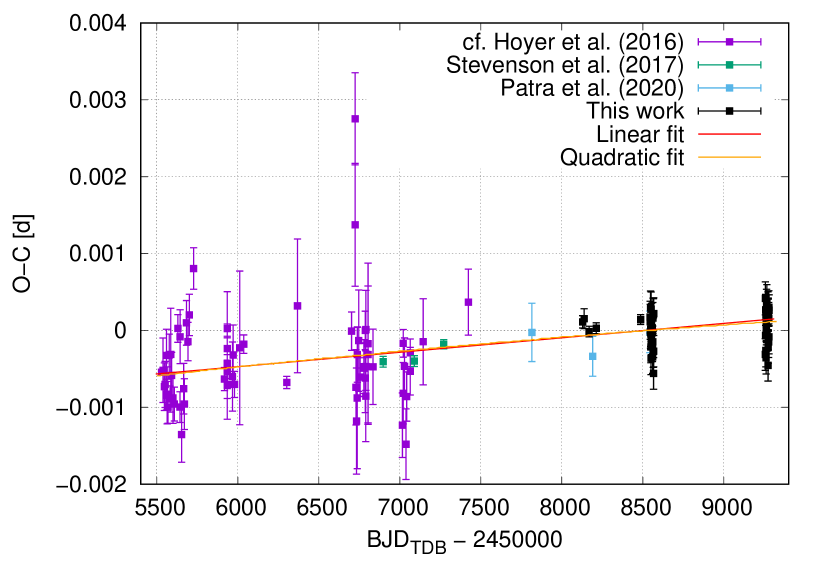

The whole O-C data-set of mid-transit times used during our analysis is presented in Fig. 6 (left-hand panel). In this graph we can see the 68 data-points, collected by Hoyer et al. (2016), the 3 data-points, observed by Stevenson et al. (2017), the 3 data-points presented by Patra et al. (2020), the 50 data-points derived from the TESS observations, plotted also separately in Fig. 6 (right-hand panel), and the 5 data-points derived from the MuSCAT2 observations in this work, i.e., 129 data-points in total. As first, these O-C data were fitted with a linear function. This fit is shown in Fig. 6 (left-hand panel). Based on the linear fit we obtained a refined linear ephemeris of:
| (5) |
Subsequently, the O-C data-set of mid-transit times was fitted with a quadratic function. This fit is also depicted in Fig. 6 (right-hand panel). We can see that the quadratic trend is not significant at the first glance. Based on this quadratic fit we obtained a quadratic ephemeris of:
| (6) |
where the quadratic coefficient is d, confirming the negligible quadratic trend in the O-C data-set of mid-transit times. Based on the Eq. 4 we can easily calculate the period change rate from . We obtained a dimensionless value of , which we can convert to ms yr-1. The result is negative, but is not significant, confirming the previous results about no detection. In comparison with the results presented by Hoyer et al. (2016), i.e., ms yr-1, derived by Stevenson et al. (2017), i.e., ms yr-1, and obtained by Patra et al. (2020), i.e., ms yr-1, our result is more precise thanks to the high quality TESS observations and to the longer time baseline. The quality of the linear and quadratic fit was expressed as Bayesian Information Criterion (), which is defined as:
| (7) |
where is the number of free parameters of the model and is the number of data-points. There is no significant difference between the two Bayesian Information Criterions, i.e., in the case of the linear fit and in the case of the quadratic fit, which means that it is not justified to use the quadratic fit.
Since we did not detect significant orbital period change rate of WASP-43b, we can adopt the values presented in Eq. 5 as a final solution for the reference mid-transit time and orbital period of the planet, i.e., and d. In comparison with the ephemeris obtained from the joint TESS and MuSCAT2 analysis (see Table 4), using the whole O-C data-set of mid-transit times we improved the parameter by a factor of 1.23 and the parameter by a factor of 1.16. This result confirms the previously published parameter values, see Table 5 for examples.
| Parameter | Value | Source |
|---|---|---|
| [] | This work | |
| [d] | This work | |
| [] | H2011 | |
| [d] | H2011 | |
| [] | H2016 | |
| [d] | H2016 |
5 Conclusions
Using the O-C data-set of mid-transit times, derived from 129 transits of WASP-43b, we have re-estimated the orbital period change rate of the exoplanet. The obtained result, ms yr-1, is consistent with a constant period well within . It confirms the previous results about no detection, but in comparison with the previous results, our result is more precise thanks to the high quality TESS observations and to the longer time baseline. By extending the observations to more than 730 days, i.e., covering a time baseline of about 10 years, we could improve the parameter by a factor of about 3.8 in comparison with the latest published result. Thus, we see no evidence to support previous claims of a decaying orbit for WASP-43b. As a by-product of the data analysis, we also derived the system parameters of WASP-43b. Several of them were refined in comparison with the previously published parameters. Thanks to combination of the high quality TESS and multi-color MuSCAT2 observations we could estimate, for example, the orbit inclination angle parameter and the combined planet-to-star radius ratio parameter precisely and without parameter degeneration. The derived parameter values are mostly in agreement with the results of existing studies. Since we did not detect significant period change rate of the planet, a new linear ephemeris of WASP-43b was derived using the whole O-C data-set of mid-transit times.
Acknowledgements
We thank Dr. S. Hoyer from the Laboratoire d’Astrophysique de Marseille (LAM) in France for the helpful discussions. We also thank the anonymous reviewer for the helpful comments and suggestions. This work was supported by the ERASMUS+ grant No. 2017-1-CZ01-KA203-035562, by the VEGA grant of the Slovak Academy of Sciences No. 2/0031/18, by an ESA PRODEX grant under contracting with the ELTE University, by the GINOP No. 2.3.2-15-2016-00003 of the Hungarian National Research, Development and Innovation Office, and by the City of Szombathely under agreement No. 67.177-21/2016. This article is based on observations made with the MuSCAT2 instrument, developed by ABC, at Telescopio Carlos Sánchez operated on the island of Tenerife by the IAC in the Spanish Observatorio del Teide. This work is partly financed by the Spanish Ministry of Economics and Competitiveness through grants No. PGC2018-098153-B-C31. This work is partly supported by JSPS KAKENHI grant Nos. JP18H01265 and JP18H05439, and JST PRESTO grant No. JPMJPR1775. This work is partly supported by JSPS KAKENHI grant No. JP17H04574. This work was partly supported by Grant-in-Aid for JSPS Fellows, grant No. JP20J21872. M.T. is supported by MEXT/JSPS KAKENHI grant Nos. 18H05442, 15H02063, and 22000005. A.C. acknowledges financial support from the State Agency for Research of the Spanish MCIU through the ”Center of Excellence Severo Ochoa” award for the Instituto de Astrophysics of Andalusia (SEV-2017-0709). We acknowledge funding from the European Research Council under the European Union’s Horizon 2020 research and innovation program under grant agreement No 694513.
Data availability
The data underlying this article will be shared on reasonable request to the corresponding author. The reduced light curves presented in this work will be made available at the CDS (http://cdsarc.u-strasbg.fr/).
References
- Astropy Collaboration et al. (2013) Astropy Collaboration et al., 2013, A&A, 558, A33
- Bailey & Goodman (2019) Bailey A., Goodman J., 2019, MNRAS, 482, 1872
- Barros et al. (2020) Barros S. C. C., Demangeon O., Díaz R. F., Cabrera J., Santos N. C., Faria J. P., Pereira F., 2020, A&A, 634, A75
- Blecic et al. (2014) Blecic J., et al., 2014, ApJ, 781, 116
- Bouma et al. (2019) Bouma L. G., et al., 2019, AJ, 157, 217
- Bouma et al. (2020) Bouma L. G., Winn J. N., Howard A. W., Howell S. B., Isaacson H., Knutson H., Matson R. A., 2020, ApJ, 893, L29
- Bradley et al. (2019) Bradley L., et al., 2019, astropy/photutils: v0.7.2, doi:10.5281/zenodo.3568287
- Chen et al. (2014) Chen G., et al., 2014, A&A, 563, A40
- Claret (2018) Claret A., 2018, A&A, 618, A20
- Csizmadia et al. (2013) Csizmadia S., Pasternacki T., Dreyer C., Cabrera J., Erikson A., Rauer H., 2013, A&A, 549, A9
- Eastman et al. (2010) Eastman J., Siverd R., Gaudi B. S., 2010, PASP, 122, 935
- Espinosa Lara & Rieutord (2011) Espinosa Lara F., Rieutord M., 2011, A&A, 533, A43
- Espinoza & Jordán (2015) Espinoza N., Jordán A., 2015, MNRAS, 450, 1879
- Esposito et al. (2017) Esposito M., et al., 2017, A&A, 601, A53
- Foreman-Mackey et al. (2013) Foreman-Mackey D., Hogg D. W., Lang D., Goodman J., 2013, PASP, 125, 306
- Foreman-Mackey et al. (2017) Foreman-Mackey D., Agol E., Ambikasaran S., Angus R., 2017, AJ, 154, 220
- Fulton et al. (2011) Fulton B. J., Shporer A., Winn J. N., Holman M. J., Pál A., Gazak J. Z., 2011, AJ, 142, 84
- Gaia Collaboration et al. (2018) Gaia Collaboration et al., 2018, A&A, 616, A1
- Gajdoš & Parimucha (2019) Gajdoš P., Parimucha Š., 2019, Open European Journal on Variable Stars, 197, 71
- Garai (2018) Garai Z., 2018, A&A, 611, A63
- Gillon et al. (2012) Gillon M., et al., 2012, A&A, 542, A4
- Gillon et al. (2014) Gillon M., et al., 2014, A&A, 562, L3
- Hebb et al. (2009) Hebb L., et al., 2009, ApJ, 693, 1920
- Hellier et al. (2009) Hellier C., et al., 2009, Nature, 460, 1098
- Hellier et al. (2011) Hellier C., et al., 2011, A&A, 535, L7
- Hoyer et al. (2016) Hoyer S., Pallé E., Dragomir D., Murgas F., 2016, AJ, 151, 137
- Jiang et al. (2016) Jiang I.-G., Lai C.-Y., Savushkin A., Mkrtichian D., Antonyuk K., Griv E., Hsieh H.-F., Yeh L.-C., 2016, AJ, 151, 17
- Kallinger et al. (2014) Kallinger T., et al., 2014, A&A, 570, A41
- Kreidberg et al. (2014) Kreidberg L., et al., 2014, ApJ, 793, L27
- Lang et al. (2010) Lang D., Hogg D. W., Mierle K., Blanton M., Roweis S., 2010, AJ, 139, 1782
- Maciejewski et al. (2016) Maciejewski G., et al., 2016, A&A, 588, L6
- Maciejewski et al. (2018) Maciejewski G., et al., 2018, Acta Astron., 68, 371
- Miralda-Escudé (2002) Miralda-Escudé J., 2002, ApJ, 564, 1019
- Murgas et al. (2014) Murgas F., Pallé E., Zapatero Osorio M. R., Nortmann L., Hoyer S., Cabrera-Lavers A., 2014, A&A, 563, A41
- Narita et al. (2019) Narita N., et al., 2019, Journal of Astronomical Telescopes, Instruments, and Systems, 5, 015001
- Oberst et al. (2017) Oberst T. E., et al., 2017, AJ, 153, 97
- Parviainen et al. (2020) Parviainen H., et al., 2020, A&A, 633, A28
- Patra et al. (2017) Patra K. C., Winn J. N., Holman M. J., Yu L., Deming D., Dai F., 2017, AJ, 154, 4
- Patra et al. (2020) Patra K. C., et al., 2020, AJ, 159, 150
- Pribulla (2012) Pribulla T., 2012, in Richards M. T., Hubeny I., eds, IAU Symposium Vol. 282, From Interacting Binaries to Exoplanets: Essential Modeling Tools. pp 279–282, doi:10.1017/S1743921311027566
- Ragozzine & Wolf (2009) Ragozzine D., Wolf A. S., 2009, ApJ, 698, 1778
- Ricci et al. (2015) Ricci D., et al., 2015, PASP, 127, 143
- Ricker (2014) Ricker G. R., 2014, Journal of the American Association of Variable Star Observers (JAAVSO), 42, 234
- Sasselov (2003) Sasselov D. D., 2003, ApJ, 596, 1327
- Stevenson et al. (2017) Stevenson K. B., et al., 2017, AJ, 153, 68
- Szabó et al. (2020) Szabó G. M., Pribulla T., Pál A., Bódi A., Kiss L. L., Derekas A., 2020, MNRAS, 492, L17
- Turner et al. (2021) Turner J. D., Ridden-Harper A., Jayawardhana R., 2021, AJ, 161, 72
- Virtanen et al. (2020) Virtanen P., et al., 2020, Nature Methods, 17, 261
- Yee et al. (2020) Yee S. W., et al., 2020, ApJ, 888, L5
- van der Walt et al. (2011) van der Walt S., Colbert S. C., Varoquaux G., 2011, Computing in Science and Engineering, 13, 22