Is Support Set Diversity Necessary for Meta-Learning?
Abstract
Meta-learning is a popular framework for learning with limited data in which an algorithm is produced by training over multiple few-shot learning tasks. For classification problems, these tasks are typically constructed by sampling a small number of support and query examples from a subset of the classes. While conventional wisdom is that task diversity should improve the performance of meta-learning, in this work we find evidence to the contrary: we propose a modification to traditional meta-learning approaches in which we keep the support sets fixed across tasks, thus reducing task diversity. Surprisingly, we find that not only does this modification not result in adverse effects, it almost always improves the performance for a variety of datasets and meta-learning methods. We also provide several initial analyses to understand this phenomenon. Our work111Implementation available at: https://github.com/ars22/fixml serves to: (i) more closely investigate the effect of support set construction for the problem of meta-learning, and (ii) suggest a simple, general, and competitive baseline for few-shot learning.
1 Introduction
The ability to learn from limited experience is a defining aspect of human intelligence. The domain of few-shot learning aims to evaluate this criterion within machine learning [10]. For few-shot learning problems, meta-learning [30] techniques have attracted increasing attention. Meta-learning methods typically construct few-shot classification tasks in an episodic manner by sampling support () and query () examples from a fixed number of classes. The objective is then to deliver an algorithm that can perform well on the query points of a task by training on only a few support samples.
Conventional wisdom is that the performance of meta-learning methods will improve as we train on more diverse tasks. Therefore, during meta-training, we typically allow a task to be constructed from any possible pair of support and query sets. In this work, we question this notion, specifically investigating the effect that support set diversity has on meta-learning. Surprisingly, we find that reducing the total number of unique support sets not only does not result in adverse effects—in most cases, it in fact yields significant performance improvements.
The main contributions of this work are as follows: (1) We propose a simple modification to the meta-learning objective that applies to a broad set of methods, in which we aim to optimize a biased objective by restricting the number of support sets used to construct tasks. (2) On multiple datasets and model architectures we empirically demonstrate the performance improvement of the learned algorithm when trained with our proposed objective. (3) Finally, we explore a framework to understand this surprising phenomenon and attempt to provide some insights into the observed gains. Our work delivers a simple, competitive baseline for few-shot learning and, more generally, investigates the role that task construction plays in meta-learning.
2 Background & Related Work
Meta-learning formulations typically rely on episodic training, wherein an algorithm is learned to adapt to a task, given its support set, so as to minimize the loss incurred on the query set. Meta-learning methods differ in terms of the algorithms they learn: Gradient-based meta-learning methods [11, 12, 23, 27, 18] consider learning gradient-based algorithms, which are typically parameterized by an initialization (possibly together with some pre-conditioning matrix). Recently, last-layer meta-learning methods [18, 22, 3, 26] have gained popularity. These methods don’t learn an optimal model parameter initialization for the task distribution but instead learn a feature extractor for the covariates in the support and query sets. The extracted support set features along with their labels are used to learn the parameters of the last layer, e.g., in a non-parametric fashion [26] or by finding the unique solution for convex problems [18, 2].
Several recent works [6, 7, 21] on few-shot learning have proposed methods that don’t directly optimize the original meta-learning objective. Instead they chose to minimize a transfer-learning based loss where a deep network is trained in a supervised manner on all the pairs present in the dataset. In contrast to episodic training, they show that a model trained without any notion of a task can be used to construct an algorithm whose performance matches or improves upon meta-learning methods across many benchmarks. Similar to these works, we propose to optimize an alternate objective for meta-learning; however, our work differs by retaining the episodic structure from the meta-learning framework but restricting the support set (and by consequence task) diversity.
In addition to using other objectives for few-shot learning, recent work aims to improve meta-learning by explicitly looking at the task structure and their relationships. Among these, Yin et al. [32] propose to handle the lack of mutual exclusiveness among different tasks through an information-theoretic regularized objective. Collins et al. [8] propose a minimax objective to make the learned algorithm task-robust, which improves the performance of the algorithm on the most difficult task in the face of a task pool with diverse difficulty. Liu et al. [20] propose to augment the set of possible tasks by augmenting the pre-defined set of classes that generate the tasks with varying degrees of rotated inputs as new classes. In addition, several popular meta-learning methods [26, 18], in order to improve the meta-test performance, change the number of ways or shots of the sampled meta-training tasks, thus increasing the complexity and diversity of the tasks. In contrast to these works, we look at the structure and diversity of tasks specifically through the lens of support set diversity, and show that, surprisingly, reducing diversity (by fixing support set) not only maintains—but in many cases significantly improves—the performance of meta-learning. Our results indicate that this simple modification to meta-learning is an effective method worthy of future study.
3 Meta-Learning with a Fixed Support Pool
We begin with some notation that we will use to re-formulate the meta-learning objective. This will allow us to introduce the concept of a support pool in a manner amenable with current meta-learning methods.
Notation. In a standard offline meta supervised learning problem, we are given a dataset with examples from different classes. A task is constructed by first choosing a subset of classes , and conditioning on , a support set and a query set are sampled i.i.d. from . The goal is to learn the parameters of an algorithm so that when given a support set , the algorithm will output a model that achieves a low loss value on the query set. We denote this loss value as a function of the algorithm parameter, support, and query set: To identify the optimal parameter of the algorithm , we optimize the objective in [A] below:
| (1) | ||||
Reformulating the meta-learning objective. We now give another view of this objective, which will motivate our proposed modified objective. Instead of sampling from the set of classes when constructing a task, we consider first sampling uniformly from , a collection of support pools. A support pool is a smaller subset of the entire dataset that contains some examples from every class in , i.e. . With , we sample a subset of classes as before and take all the examples from that are of the classes in . This set of examples is now our support set which we denote by . With the classes determined, we can then sample the query set of examples from class the same way as described previously. In this view, the marginal distribution of the support query set pair is exactly the same as that of discussed before. As a result, we can rewrite our meta-learning objective as in (1)[B].
This reformulation prompts us to first check how big the collection of support pools typically is. In the most unconstrained form, can contain all possible subsets of a dataset where we have at least one sample from every class . However, most meta-learning methods only train on episodic tasks where the support is of a specific configuration, i.e., the support of each task is comprised of exactly ways (classes) with each class having shots (examples). For instance, when training on miniImagenet [31] -way -shot () tasks, all tasks that are sampled consist of exactly shots from each of the classes. Hence, it also makes sense to limit to only support pools that obey a certain structure. In this work, we consider to consist only of subsets of that have exactly samples from each class i.e. . The meta-training set of miniImagenet [24] has 64 classes with 600 examples each, resulting in support pools. This makes us wonder: Is this astronomically large number of support pools necessary or possibly redundant to achieve good meta-test performance? Can we use a much smaller number of support pools instead?
Fixing the support pool. Motivated from the questions above, we take the most extreme reduction approach: before training begins, we randomly construct one support pool and let (just this single support pool) and solve for the corresponding optimization problem:
| (2) |
Note that the expectation over is removed because there is only a single possible realization of the random support pool. In terms of the total number of different possible support sets that the algorithm being learned can see, we have also achieved a reduction factor of times for the aforementioned miniImagenet example. In the rest of the paper, we first show the performance obtained by optimizing this reduced objective (2) for some of the best-performing meta-learning methods on multiple meta-learning problems and/or with different model architectures. We then make an initial attempt at understanding the effectiveness of using this fixed support pool objective.
4 Experiments
We now aim to understand the differences in generalization performance between the algorithm learned by optimizing (2), i.e. our proposed objective (which we denote fix-ml), and the algorithm obtained by optimizing the original meta-learning objective (1) (which we denote ml).
For every fix-ml experiment, we randomly sample samples (shots) from each class in the dataset to form the support pool , which is then fixed throughout training. Here, different runs of fix-ml on the exact same problem and meta-learning method can use different (but fixed) support pools. Later in this section, we will discuss how this randomness affects meta-test performance over multiple fix-ml runs. For an unbiased estimation and a fair comparison, when we evaluate a fix-ml learned algorithm on the meta-validation or meta-test set, we compute the loss and accuracy using the objective given in (1) (i.e., an average over all possible support pools), just as we would for the ml learned algorithm.
To fully evaluate the performance differences, we compare fix-ml and ml along three axes:
-
1.
Meta-learning methods: We focus our initial experiments on protoypical-networks (PN) [26] which uses a non-parametric last layer solver, as Protonets is a highly competitive ml approach, and also has the benefit of training faster and with less memory than competitors such as SVM [18], Ridge Regression (RR) [3]. However, we also experiment with SVM and RR-based solvers to confirm that the trends observed with Protonets generalize to these methods. As initialization-based methods are harder to optimize for highly over-parameterized models, we defer such evaluations to future work.
-
2.
Datasets: Our study mainly uses two of the most widely-used benchmarks in few-shot learning: (i) miniImagenet (mini) [31], which consists of 100 classes of images, split into 64 train, 16 validation and 20 test, and (ii) CIFAR-FS (cifar) [3] with an identical split but with images. Additionally for the SVM method we elect to compare on the more difficult FC-100 (FC) dataset, as the SVM-based solver has achieved significantly superior performance on this benchmark [18].
-
3.
Architectures: We conduct our main experiments using Resnet-12, as many meta-learning methods [2, 22] have relied on this architecture to achieve good performance. Additionally, we experiment with another wider but shallower over-parameterized architecture, WideResNet-16-10 [33] (also used by [25]), and Conv64, which was used by some initial works in meta-learning [11, 26].
Main Results.
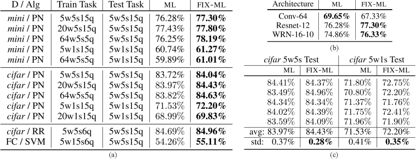
Figure 1(a) consolidates the results of our experiments on different datasets with a myriad of training task configurations. Surprisingly, contrary to our intuition about task diversity, we can clearly see that optimizing the fix-ml objective performs similarly or in many cases better with respect to its ml counterpart. In all the cases except for the cifar dataset, we evaluate the validation and test accuracies on randomly drawn tasks consisting of novel classes and for each of them we observe a confidence interval of around their respective means. For cifar, since the performance improvements are lower, we evaluate on tasks instead and observe a interval of (around the reported mean) which confirms the significance of the improvement.
Specifically, we see that on all of the mini and cifar 5w1s and 5w5s evaluations, Protonets trained with fix-ml achieve better performance. In addition, for each of these evaluations, we consider training with different number of ways and shots as proposed in [26, 18]. Our results also confirm that fix-ml is better for a range of meta-training specifics. Besides, for other meta-learning methods like SVM and RR, fixing the support pool can also improve performance. For all the experiments in Figure 1(a) we use the Resnet-12 backbone. In order to further validate our findings, we show mini-5w5s meta test results on two other architectures in Figure 1(b). WRN-16-10 has roughly 50% more parameters than Resnet-12 and we see that fix-ml continues to perform better than ml in this over-parameterized regime. On the other hand, it seems that fixing the support pool for shallower backbones like Conv64 hinders the meta-test performance. For this we hypothesize that fix-ml is effective for over-parameterized models and algorithms but less so for shallower models with fewer parameters. Further analysis on how model architecture and over-parameterization affects fix-ml is a future research direction.
Recall that earlier in this section, we suspected that fixing the support pool randomly prior to the start of training may induce higher variance in the final meta-test performance over different runs. From the observations in Figure 1(c), we confirm that this is not true. We compare fix-ml and ml on cifar-5w5s and cifar-5w1s over five different runs each, where for every run of fix-ml a different random support pool was sampled and then fixed. We can clearly see that the performance standard deviation is not only not worse but actually better than ml. Finally, in Figure 3(a) we see that Protonets trained using fix-ml objective achieves competitive results on mini-5w5s when compared with other other meta-learning methods and with a simple transfer learning method [6] devoid of any self-supervised learning [21] tricks or a transductive setting [14].
Implementation.
We follow the learning rate schedule and data augmentation scheme of [18] and use a task batch size of 4-8 when training with lower number of ways (e.g., ) due to observed improvements in convergence and generalization. Additionally, we experiment with varying number of query points per class (in a single task). We observe that for some cases in Figure 1(a) this further improves the advantage of fix-ml over ml.
5 Discussion
To understand the improved meta-test performance of the fix-ml-learned algorithms, we first analyze their performance on the meta-training set. Evaluating the fix-ml-learned algorithm’s performance averaged over all possible support pools (equivalent to the standard ml training loss) is important because, by the generalization theory using uniform convergence bounds (e.g. VC dimension, Rademacher complexity [1]), the test loss tracks training loss more closely with more training samples. In the case of meta-learning, the “samples” are tasks in the form of pairs. Therefore, we see that an algorithm’s ml-training loss which considers all possible pairs, should track the algorithm’s loss on the meta-test set more reliably than the fix-ml training loss which uses only a single support pool (inducing much fewer pairs).


Naively, one might think that because fix-ml is optimized on a single fixed support pool, the training loss on any other support pool would be much worse. To verify this idea, we re-evaluate the fix-ml-learned algorithms 1) over other fixed support pools by replacing in (2) with ; 2) on the original meta-learning objective (1)[B] by averaging over all possible support pools (because of the large number of possible support pools, we estimate this average using a very large number of sampled tasks). We conduct this evaluation for Protonet on cifar-5w5s and cifar-5w1s tasks, for all the trained algorithm snapshots over the entire training epochs. Here, the random class set in (1)[B] is set to always contain exactly classes () in order to match the meta-test scenario. The results are shown in Figure 3(b),(c). As we see in both plots, despite optimizing for one fixed support pool (blue curve), the training losses of other support pools (green curves) and the ml training loss (red curve) are all decreasing consistently in the same trend as the blue curve throughout the entire optimization trajectory. To understand this consistent decrease, we note that the gradient of fix-ml objective is a biased gradient of the original ml objective. When the gradient bias is not too large, stochastic gradient descent using a biased gradient can still lead to a reduction in objective loss and convergence [4], which is what we observe for the ml objective when using biased stochastic fix-ml gradients.
However, this does not give us a complete picture for meta-training. Even though ml training loss is considerably reduced for the fix-ml-learned algorithm, we need to compare this value against ml-training loss of the corresponding ml-learned algorithm to understand the meta-test performance difference. In Figure 3(c), we compare the end-of-training fix-ml solutions with the corresponding ml solutions using the ml training objective (1)[B] on 4 different dataset/task configurations. We see that fix-ml still consistently achieves higher ml-training losses than their ml counterparts. With a relatively lower ml test loss but a much higher ml training loss, the fix-ml solution must have a smaller generalization gap than that of the ml solution. Since there isn’t a single best way to understand neural networks’ generalization gap, we look at some of the recently proposed metrics:
1) Sharpness of the training loss landscape: A popular hypothesis (dating back to [13]) is that the flatness of the training loss landscape is correlated with (and possibly leads to) a smaller generalization gap [17, 5]. Several sharpness metrics based on this hypothesis were called into question by [9], showing that a functionally equivalent neural network with differently scaled parameters could have arbitrarily different sharpness according to these metrics. However, it was argued in [16] that even though sharp minima with similar test performance as flat minima do exist, stochastic gradient descent will not converge to them. While further understanding sharpness’s relationship with generalization gap is still an ongoing research topic, we still consider two sharpness analyses here.
1a) Sharpness visualization using 1d interpolation plots was first proposed by [17] and also used by [15] to compare the flatness of two different solutions’ training loss landscape when explaining the two solutions’ generalization gap differences. For two models with the same neural architecture but different weights, training and test loss are evaluated at model parameters that are different linear interpolations of the two models’ weights. In our case, we interpolate between the parameters of end-of-training fix-ml-learned algorithm and ml-learned algorithm from Protonet for miniImagenet 5w5s. This result is shown in Figure 3(a),(b). In 3(a), we see that fix-ml is located at a relatively “sharper” minima than ml despite having a smaller generalization gap. This is inconsistent with observations in [17, 15] possibly because in our case, the loss landscape between meta-train and meta-test are not necessarily shifted versions of each other (confirmed also in Figure 3(b)). Instead, we see that the trends of these two graphs align well with each other. Therefore, we cannot solely rely on 1d visualization-based sharpness analysis to explain the generalization gap.

1b) In addition to visualizations, quantitative measures of the training loss landscape sharpness has also been used. Specifically, one notion of the loss landscape sharpness is in the curvature of the loss function. This is typically measured by the maximum eigenvalue [19] or the trace of the Hessian matrix () [16] for the parameters at the end of training . However, directly computing accurately is both computationally expensive and memory-wise “impossible" for over-parameterized models like Resnet-12. Thus, is typically approximated with the Fisher information matrix () at the same parameter [29]. can be easily estimated without constructing the entire matrix . However, is only equal to when the parameters are the true parameters of the training set (in practice, achieve training loss extremely close to ). On the other hand, this approximation is very crude when the training loss is much larger than in the case of fix-ml (Figure 3(c)). Hence, for fix-ml’s parameters cannot be accurately estimated using . As a result, for our analysis, this approach is not readily applicable.
2) Another quantitative measure which approximates the Takeuchi Information Criterion (TIC) [28] was empirically shown to correlate more with the generalization gap as compared to measures of the loss landscape’s flatness [29]. Specifically, Thomas et al. (2020) proposes the quantity , where is the uncentered covariance matrix of the gradient with respect to the training data distribution. To evaluate how well this measure tracks the generalization gap difference between fix-ml and ml, we evaluate this approximate TIC value for three pairs of ml and fix-ml-learned algorithms in Figure 3(d). We see that for all three datasets, ml has both higher and larger generalization gap than its fix-ml counterpart, indicating some possible correlation between these two. Thus it would be interesting to understand what intuitive property of the solutions is captured by this quantity and why optimizing the fix-ml objective leads to solutions with lower .
6 Conclusion
In this paper, we have proposed a simple yet effective modification of the meta-learning objective. We begin by re-formulating the traditional meta-learning objective, which motivates our approach of reducing the support set diversity. Then, we experimentally show that for a variety of meta-learning methods, datasets, and model architectures, the algorithms learned using our objective result in superior generalization performance relative to the original objective. We analyze this improvement by understanding the optimization loss and the generalization gap separately. While the optimization loss trade-off is easier to reason about using our framework, the generalization gap is still not fully understood based on several initial analyses, which we hope would pave the way for future work in this area.
References
- Bartlett and Mendelson [2002] P. L. Bartlett and S. Mendelson. Rademacher and gaussian complexities: Risk bounds and structural results. Journal of Machine Learning Research, 3(Nov):463–482, 2002.
- Bertinetto et al. [2018a] L. Bertinetto, J. F. Henriques, P. H. Torr, and A. Vedaldi. Meta-learning with differentiable closed-form solvers. arXiv preprint arXiv:1805.08136, 2018a.
- Bertinetto et al. [2018b] L. Bertinetto, J. F. Henriques, P. H. S. Torr, and A. Vedaldi. Meta-learning with differentiable closed-form solvers. arXiv preprint arXiv:1805.08136, 2018b.
- Bottou et al. [2018] L. Bottou, F. E. Curtis, and J. Nocedal. Optimization methods for large-scale machine learning. Siam Review, 60(2):223–311, 2018.
- Chaudhari et al. [2019] P. Chaudhari, A. Choromanska, S. Soatto, Y. LeCun, C. Baldassi, C. Borgs, J. Chayes, L. Sagun, and R. Zecchina. Entropy-sgd: Biasing gradient descent into wide valleys. Journal of Statistical Mechanics: Theory and Experiment, 2019(12):124018, 2019.
- Chen et al. [2019] W.-Y. Chen, Y.-C. Liu, Z. Kira, Y.-C. F. Wang, and J.-B. Huang. A closer look at few-shot classification. arXiv preprint arXiv:1904.04232, 2019.
- Chen et al. [2020] Y. Chen, X. Wang, Z. Liu, H. Xu, and T. Darrell. A new meta-baseline for few-shot learning. arXiv preprint arXiv:2003.04390, 2020.
- Collins et al. [2020] L. Collins, A. Mokhtari, and S. Shakkottai. Task-robust model-agnostic meta-learning. Advances in Neural Information Processing Systems, 33, 2020.
- Dinh et al. [2017] L. Dinh, R. Pascanu, S. Bengio, and Y. Bengio. Sharp minima can generalize for deep nets. arXiv preprint arXiv:1703.04933, 2017.
- Fei-Fei et al. [2006] L. Fei-Fei, R. Fergus, and P. Perona. One-shot learning of object categories. IEEE transactions on pattern analysis and machine intelligence, 28(4):594–611, 2006.
- Finn and Levine [2017] C. Finn and S. Levine. Meta-learning and universality: Deep representations and gradient descent can approximate any learning algorithm. arXiv preprint arXiv:1710.11622, 2017.
- Finn et al. [2018] C. Finn, K. Xu, and S. Levine. Probabilistic model-agnostic meta-learning. In Advances in Neural Information Processing Systems, pages 9516–9527, 2018.
- Hochreiter and Schmidhuber [1997] S. Hochreiter and J. Schmidhuber. Flat minima. Neural Computation, 9(1):1–42, 1997.
- Hu et al. [2020] Y. Hu, V. Gripon, and S. Pateux. Leveraging the feature distribution in transfer-based few-shot learning. arXiv preprint arXiv:2006.03806, 2020.
- Izmailov et al. [2018] P. Izmailov, D. Podoprikhin, T. Garipov, D. Vetrov, and A. G. Wilson. Averaging weights leads to wider optima and better generalization. In 34th Conference on Uncertainty in Artificial Intelligence 2018, UAI 2018, pages 876–885. Association For Uncertainty in Artificial Intelligence (AUAI), 2018.
- Jastrzębski et al. [2017] S. Jastrzębski, Z. Kenton, D. Arpit, N. Ballas, A. Fischer, Y. Bengio, and A. Storkey. Three factors influencing minima in sgd. arXiv preprint arXiv:1711.04623, 2017.
- Keskar et al. [2016] N. S. Keskar, D. Mudigere, J. Nocedal, M. Smelyanskiy, and P. T. P. Tang. On large-batch training for deep learning: Generalization gap and sharp minima. arXiv preprint arXiv:1609.04836, 2016.
- Lee et al. [2019] K. Lee, S. Maji, A. Ravichandran, and S. Soatto. Meta-learning with differentiable convex optimization. In Proceedings of the IEEE Conference on Computer Vision and Pattern Recognition, pages 10657–10665, 2019.
- Li et al. [2018] H. Li, Z. Xu, G. Taylor, C. Studer, and T. Goldstein. Visualizing the loss landscape of neural nets. In Advances in Neural Information Processing Systems, pages 6389–6399, 2018.
- Liu et al. [2020] J. Liu, F. Chao, and C.-M. Lin. Task augmentation by rotating for meta-learning. arXiv preprint arXiv:2003.00804, 2020.
- Mangla et al. [2020] P. Mangla, N. Kumari, A. Sinha, M. Singh, B. Krishnamurthy, and V. N. Balasubramanian. Charting the right manifold: Manifold mixup for few-shot learning. In The IEEE Winter Conference on Applications of Computer Vision, pages 2218–2227, 2020.
- Oreshkin et al. [2018] B. N. Oreshkin, P. Rodriguez, and A. Lacoste. Tadam: Task dependent adaptive metric for improved few-shot learning. arXiv preprint arXiv:1805.10123, 2018.
- Rajeswaran et al. [2019] A. Rajeswaran, C. Finn, S. M. Kakade, and S. Levine. Meta-learning with implicit gradients. In Advances in Neural Information Processing Systems, pages 113–124, 2019.
- Ravi and Larochelle [2016] S. Ravi and H. Larochelle. Optimization as a model for few-shot learning. 2016.
- Rusu et al. [2018] A. A. Rusu, D. Rao, J. Sygnowski, O. Vinyals, R. Pascanu, S. Osindero, and R. Hadsell. Meta-learning with latent embedding optimization. arXiv preprint arXiv:1807.05960, 2018.
- Snell et al. [2017] J. Snell, K. Swersky, and R. Zemel. Prototypical networks for few-shot learning. In Advances in neural information processing systems, pages 4077–4087, 2017.
- Sung et al. [2018] F. Sung, Y. Yang, L. Zhang, T. Xiang, P. H. Torr, and T. M. Hospedales. Learning to compare: Relation network for few-shot learning. In Proceedings of the IEEE Conference on Computer Vision and Pattern Recognition, pages 1199–1208, 2018.
- Takeuchi [1976] K. Takeuchi. The distribution of information statistics and the criterion of goodness of fit of models. Mathematical Science, 153:12–18, 1976.
- Thomas et al. [2020] V. Thomas, F. Pedregosa, B. Merriënboer, P.-A. Manzagol, Y. Bengio, and N. Le Roux. On the interplay between noise and curvature and its effect on optimization and generalization. In International Conference on Artificial Intelligence and Statistics, pages 3503–3513. PMLR, 2020.
- Thrun and Pratt [1998] S. Thrun and L. Pratt. Learning to Learn. Springer, 1998.
- Vinyals et al. [2016] O. Vinyals, C. Blundell, T. Lillicrap, D. Wierstra, et al. Matching networks for one shot learning. In Advances in neural information processing systems, pages 3630–3638, 2016.
- Yin et al. [2019] M. Yin, G. Tucker, M. Zhou, S. Levine, and C. Finn. Meta-learning without memorization. arXiv preprint arXiv:1912.03820, 2019.
- Zagoruyko and Komodakis [2016] S. Zagoruyko and N. Komodakis. Wide residual networks. arXiv preprint arXiv:1605.07146, 2016.