\ul
InvGC: Robust Cross-Modal Retrieval by Inverse Graph Convolution
Abstract
Over recent decades, significant advancements in cross-modal retrieval are mainly driven by breakthroughs in visual and linguistic modeling. However, a recent study shows that multi-modal data representations tend to cluster within a limited convex cone (as representation degeneration problem), which hinders retrieval performance due to the inseparability of these representations. In our study, we first empirically validate the presence of the representation degeneration problem across multiple cross-modal benchmarks and methods. Next, to address it, we introduce a novel method, called InvGC, a post-processing technique inspired by graph convolution and average pooling. Specifically, InvGC defines the graph topology within the datasets and then applies graph convolution in a subtractive manner. This method effectively separates representations by increasing the distances between data points. To improve the efficiency and effectiveness of InvGC, we propose an advanced graph topology, LocalAdj, which only aims to increase the distances between each data point and its nearest neighbors. To understand why InvGC works, we present a detailed theoretical analysis, proving that the lower bound of recall will be improved after deploying InvGC. Extensive empirical results show that InvGC and InvGC w/LocalAdj significantly mitigate the representation degeneration problem, thereby enhancing retrieval performance.
Our code is available at link.
1 Introduction
Cross-modal retrieval (CMR) Wang et al. (2021); Yu et al. (2023); Kim et al. (2023), which aims to enable flexible retrieval across different modalities, e.g., images, videos, audio, and text, has attracted significant research interest in the last few decades. The goal of CMR is to learn a pair of encoders that map data from different modalities into a common space where they can be directly compared. For example, in text-to-video retrieval, the objective is to rank gallery videos based on the features of the query text. Recently, inspired by the success in self-supervised learning Radford et al. (2021), significant progress has been made in CMR, including image-text retrieval Radford et al. (2021); Li et al. (2020); Wang et al. (2020a), video-text retrieval Chen et al. (2020); Cheng et al. (2021); Gao et al. (2021); Lei et al. (2021); Ma et al. (2022); Park et al. (2022); Wang et al. (2022a, b); Zhao et al. (2022); Wang and Shi (2023); Wang et al. (2023), and audio-text retrieval Oncescu et al. (2021), with satisfactory retrieval performances.
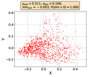
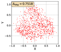
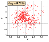
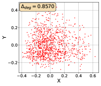
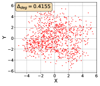
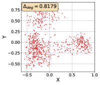
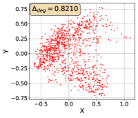
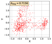
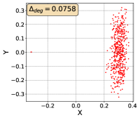
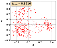
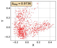
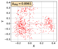
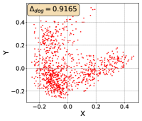
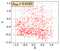
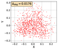
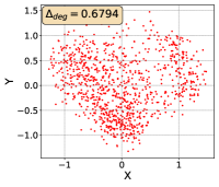
However, Liang et al. (2022) demonstrate that the current common learning paradigm of CMR leads to the representation degeneration problem, which concentrates all the representations in a small (convex) cone Gao et al. (2019); Zhang et al. (2020) in image-text retrieval and the cosine similarity between any two points is positive, as shown in Figure 1(a). Consequently, retrieval performance will be significantly affected Radovanovic et al. (2010); Gao et al. (2019). Due to the limitation of space, detailed related works are presented in Appendix A.
In this paper, to step forward in addressing representation degeneration problem and further improve the retrieval performance, we first empirically test whether it is prevalent across various cross-modal retrieval models and datasets, including video, image, text, and audio. We found that the representations of MSCOCO generated by CLIP are gathered in a very narrow cone in the embedding space, proving the existence of representation degeneration problem, as shown in Figure 1(a). This case does not stand alone since similar observations are observed across several cross-modal retrieval models and datasets as shown in Section C.3.
Next, to model how severe the representation degeneration problem is and the relationship between this problem and the retrieval performance, drawing inspiration from previous work Gao et al. (2019); Zhang et al. (2020); Yu et al. (2022); Liang et al. (2022); Yang et al. (2022); Huang et al. (2021), we define it in CMR as the average similarity between each point and its nearest neighbor in the gallery set, as shown in Equation 2. We observe that the scores are very high across different datasets and methods. They are able to model this problem as a high score always leads to more concentrated data distribution as shown in Section C.3.
While CMR has suffered from this problem, on the other side, the graph convolution Kipf and Welling (2017) and average pooling Boureau et al. (2010), which are widely employed in graph neural networks Gilmer et al. (2017); Kipf and Welling (2017); Velickovic et al. (2018) and deep neural networks He et al. (2016); Yu et al. (2023), respectively, are designed to move the representations closer to each other if they are semantically similar Baranwal et al. (2023). It might lead to the emergence of representation degeneration problem.
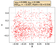
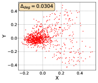
Drawing inspiration from the graph convolution and average pooling, we propose a novel method, InvGC, which separates representations by performing the graph convolution inversely to separate representations with a bigger margin as shown in Figure 1(a). Specifically, different from the vanilla graph convolution, considering one modality, InvGC separates representations by subtracting the representation of the neighboring nodes from each node, instead of aggregating them as,
| (1) |
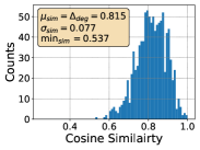
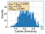
where and are the updated and the original representations, is the similarity between the -th and -th data, and is a predefined hyperparameter. As shown in Figure 1, InvGC better scatter representations and alleviates representation degeneration problem. Moreover, the histogram of similarity between any two points is more balanced with InvGC, as shown in Figure 1. To boost the effectiveness and efficiency of InvGC, we propose an advanced adjacency matrix LocalAdj that directs InvGC w/LocalAdj to focus on the nearest neighbors of each data point instead of considering all the data points.
To evaluate the effectiveness of InvGC and InvGC w/LocalAdj, we conducted experiments on eight cross-modal benchmarks Xu et al. (2016); Chen and Dolan (2011); Fabian Caba Heilbron and Niebles (2015); Hendricks et al. (2017); Lin et al. (2014); Plummer et al. (2017); Kim et al. (2019); Drossos et al. (2020). Experimental results show that InvGC alleviates representation degeneration problem across different datasets and methods and improves retrieval performance as a by-product.
In summary, our contributions are as follows111The code is released at link.:
-
•
We are the first to formalize the definition of representation degeneration in cross-modal retrieval and perform a theoretical analysis of the relationship between representation degeneration problem and retrieval performance.
-
•
Inspired by the graph convolution, we propose the first post-processing method in cross-modal retrieval, namely InvGC, to alleviate representation degeneration problem without any training process or additional data.
-
•
We design an adjacency matrix, called LocalAdj, for the graph convolution, which leverages only the nearest neighbors of each data point instead of all the data. InvGC with LocalAdj, namely InvGC w/LocalAdj. It is shown to be more effective and efficient.
-
•
Extensive experiments show that InvGC and InvGC w/LocalAdj alleviate representation degeneration problem and improve retrieval performance as a by-product.
2 Preliminaries
2.1 Task Definition
In this paper, we focus on the representation degeneration problem in cross-modal retrieval Wang et al. (2020b). Two modalities are denoted as and . is the query modality, while is the gallery modality. The (test) gallery, denoted , contains all the representations of the (test) gallery data, where is the size. The query set is , where is the number of queries. Usually, in cross-modal retrieval, the gallery data does not overlap with the training data. Additionally, as InvGC requires training (or validation) data to address the representation degeneration problem, we define the set of representations of training (or validation) query and gallery data as and , respectively, where and are the size of the training (or validation) query and gallery set, respectively. The similarity between two embeddings and is defined as , where could be some measure of distance.
2.2 Representation Degeneration in Cross-modal Retrieval
Taking inspiration from Liang et al. (2022), we define the representation degeneration problem as the average similarity of pairs that are closest to each other,
| (2) |
where is the closest data point to while is the number of data points. A higher score, as shown in Section C.3, indicates a more severe representation degeneration issue, with each data point being closer to its nearest neighbors in the set.
To understand the relationship between the degeneration score (Equation 2) and the retrieval performance, we present the following theorems.
Theorem 1.
Let be any point in , be the nearest neighbor of and be the dimension of the representation. Given a query point that is semantically similar to and sampled from , which follows an independent and identical uniform distribution in , the probability of a query point to successfully retrieve , denoted , is bounded by,
where .
Corollary 2.
The ratio between the probability of successful retrieval of any two different neighborhood radii, namely and , is
Due to space limitation, the proofs are deferred to Section D.1.
Remark 1.
These theorems show that a high similarity of the nearest neighbor, i.e., smaller , leads to an exponentially lower probability for successful retrieval. Therefore, a higher score leads to bad retrieval performance.
3 InvGC
To alleviate the representation degeneration problem and further boost the retrieval performance, we design a post-processing method, called InvGC, which does not need any additional training.
Our idea is generally based on the mathematical principles laid out in Equation 1 and Figure 1, where the inverse version of graph convolution is able to decrease the similarity between data points and their neighbors. For the sake of clear representation, we use the cosine similarity as the similarity metric in this section following Luo et al. (2022), as it is the most common practice in cross-modal retrieval222InvGC can be easily migrated to other similarity metrics adopted by different retrieval methods Croitoru et al. (2021); Liu et al. (2019).. The formal definition of InvGC is presented in Section 3.3.
3.1 Mathematical Intuition
InvGC originates from graph convolution, which is widely employed in graph neural networks Kipf and Welling (2017); Gilmer et al. (2017); Velickovic et al. (2018).
Specifically, graph convolution will concentrate all the embeddings of similar nodes which might lead to the concentration of similarity de la Pena and Montgomery-Smith (1995) and the data degeneration problem Baranwal et al. (2023). On the other side, a similar operation, average pooling, has been employed in computer vision He et al. (2016); Wang and Shi (2023). Average pooling will aggregate the features that are location-based similar333The details of graph convolution and average pooling discussed in this study are deferred to the Sections B.1 and B.2, respectively..
As a result, graph convolution and average pooling concentrate the representation of all the similar nodes and force them to become very similar to each other, potentially leading to representation degeneration problem. This observation inspires us to pose the following research question:
Can the issue of representation degeneration problem in cross-modal retrieval be alleviated by conducting inverse graph convolution (InvGC)?
To answer this question, we first give an inverse variant of graph convolution as follows,
| (3) |
where is the adjacency matrix for the data in the gallery set. Since the adjacency matrix is not available, to encourage separating the nearest neighbor in terms of the similarity score of each node, we choose with detailed discussion in Section 3.2. Therefore, based on the inverse graph convolution, we propose the basic setting of InvGC as shown in Equation 1, which only considers one modality. We notice that it is able to alleviate the representation degeneration problem as shown in Figure 1.
Note that the ultimate goal of InvGC is to reduce score of the distribution of the representation of the gallery instead of merely the gallery set , which can be regarded only as a sampled subset of the distribution with very limited size in practice. Therefore, the best approximation of the distribution is the training (or validation) gallery set since it is the largest one we can obtain444In practice, the test queries are invisible to each other as the queries do not come at the same time. So the size of the query set is equal to 1..
Similarly, the distribution of the query set is theoretically expected to be similar to that of as a basic assumption in machine learning Bogolin et al. (2022). A detailed explanation of the claims is included in Section B.3. Moreover, as CMR needs to contrast the data points from both modalities, we utilize the (train or validation) gallery set and the (train or validation) query set to better estimate the hidden distribution as shown in Equation 4,
| (4) |
where and are two hyperparameters, and is the adjacency matrices between every pair of embedding from and and that from and , respectively.
To the best of our knowledge, InvGC is the first to utilize the (inverse) graph convolution for separating the representation of data. Instead of the commonly used capability of aggregation and message passing, we introduce an inverse variant of convolution that separates data representations compared to the vanilla graph convolution.
3.2 Constructing Adjacency matrix
Next, we need to establish the graph structure, i.e., build the adjacency matrix and , since there is no natural graph structure in the dataset. The simplest idea will be that the edge weight between and equals 1, i.e., , if the cosine similarity between and , i.e., , is larger than 0 (or some thresholds). InvGC with this form of the adjacency matrix is an inverse variant of average pooling. It serves as a baseline in this study, denoted as AvgPool.
However, this scheme is not capable to reflect the degree of the similarity between and since it cannot precisely depict the relation between different data points.
As the magnitude of directly controls how far will go in the opposite direction of , a greedy design will be using the similarity score between them as the edge weight, i.e., .
Therefore, we can calculate the adjacency matrix , which contains the similarity score between every pair of embedding from and , respectively. Specifically, the -entry of follows,
| (5) |
Similarly, the matrix containing the similarity score between every pair of embedding from and is calculated as follows,
| (6) |
Now, with the well-defined and , we can finally perform InvGC to alleviate representation degeneration problem.
As shown in Theorem 1, given any data point, the similarity of the nearest neighbor in the representation space is critical to retrieval performance. Inspired by this, when performing the inverse convolution on a node, we force InvGC to pay attention to those most similar nodes to it. This can be achieved by assigning edge weight only to the nodes having the top percent of the largest similarity scores relative to the given node. Specifically, each entry of and in this case is calculated as follows,
| (7) |
| (8) |
where is the value of -percentage largest similarity between node and all the nodes in . The same approach applies to as well. We denote this refined adjacency matrix as LocalAdj since it focuses on the local neighborhoods of each node.
3.3 Formal Definition of InvGC
With the well-formed adjacency matrices , we formally define InvGC to obtain the updated embedding of , denoted as , in a matrix form as,
| (9) |
where normalizes a matrix with respect to rows, which is employed for uniformly distributing the intensity of convolution when cosine similarity is used and should be removed when adopting other similarity metrics and the adjacency matrices and can be calculated as Equations 5, 6 and 7. Note that, compared to Equation 4, we separate the convolution on and to pursue more robust results, for avoiding the distribution shifts between and due to the imperfection of the representation method.
In summary, InvGC, as shown in Equation 9, is a brand new type of graph operation performed on the specifically designed graph structures (adjacency matrix) of data points in the cross-modal dataset. It helps alleviate the representation degeneration problem by separating data points located close to each other in the representation space.
After obtaining , the similarity between the -th gallery points and a query point is calculated as .
| Text-to-Video Retrieval | Video-to-Text Retrieval | |||||
| MeanSim | MeanSim@1 | MeanSim@10 | MeanSim | MeanSim@1 | MeanSim@10 | |
| CLIP | 0.4717 | 0.8211 | 0.7803 | 0.5162 | 0.9029 | 0.8596 |
| CLIP w. InvGC | 0.4693 | 0.8142 | 0.7738 | 0.5137 | 0.8972 | 0.8542 |
| Difference to the baseline (%) | 0.51 | 0.84 | 0.83 | 0.48 | 0.63 | 0.63 |
| CLIP w. InvGC w/LocalAdj | 0.4646 | 0.8059 | 0.7647 | 0.5105 | 0.8924 | 0.8477 |
| Difference to the baseline (%) | 1.51 | 1.85 | 2.00 | 1.09 | 1.16 | 1.38 |
| Text-to-Video Retrieval | Video-to-Text Retrieval | |||||
| MeanSim | MeanSim@1 | MeanSim@10 | MeanSim | MeanSim@1 | MeanSim@10 | |
| CLIP | 0.1516 | 0.3282 | 0.3138 | 0.1516 | 0.3213 | 0.3009 |
| CLIP w. InvGC | 0.1500 | 0.3245 | 0.3101 | 0.1511 | 0.3198 | 0.2994 |
| Difference to the baseline(%) | 1.06 | 1.13 | 1.18 | 0.33 | 0.47 | 0.50 |
| CLIP w. InvGC w/LocalAdj | 0.0635 | 0.2214 | 0.2035 | 0.0921 | 0.2414 | 0.2208 |
| Difference to the baseline(%) | 58.11 | 32.54 | 35.15 | 39.25 | 24.87 | 26.62 |
4 Experiments
We conduct a series of experiments to demonstrate that InvGC can efficiently alleviate the representation degeneration problem in a post-hoc manner. We compare InvGC and InvGC w/LocalAdj with the baseline performance produced by the representation model adopted. We also introduce the inverse version of average pooling, namely AvgPool, as another baseline. A series of ablation studies indicate that InvGC addresses the representation degeneration problem by reducing the similarity between points in the gallery set and is not sensitive to hyperparameters and the amount of training data.
4.1 Experimental and implementation settings
The implementation of InvGC exactly follows Equation 9 with the adjacency matrix defined in Equations 5 and 6 and a separate pair of tuned hyperparameters and for each retrieval model of each dataset. To balance the edge weight in and and make sure the scale of weights is stable, they subtract their average edge weights, respectively.
The only difference between InvGC w/LocalAdj and InvGC is the adjacency matrix applied. Instead of the ones from Equations 5 and 6, we apply and defined in Equations 7 and 8. We choose the value of to be 1 (i.e., top 1% nearest neighbors) throughout the study while the proposed method is very robust to the value of the . There is a large range of reasonable values that can boost the performance, proved by the ablation study in Section 4.3.
AvgPool is the simplest variant of inverse graph convolution with binary adjacency matrix where the edge weight between a pair of nodes is 1 if they are neighbors, or 0 otherwise. Then, following the approach in LocalAdj, we update the embeddings using only the top percent of nearest neighbors. To provide a more comprehensive benchmark, we pick four values of from to . Note that we also independently tune and for AvgPool to make sure the evaluation is fair. The comparison with AvgPool validates not only the effectiveness of InvGC but also the importance of the similarity-based adjacency matrix. The detailed setting is included in Section C.4.
4.2 Datasets and evaluation metrics
While we mainly focus our experiments on standard benchmarks for text-image retrieval, i.e., MSCOCO Lin et al. (2014) and Flickr30k Plummer et al. (2017), we also explore the generalization of InvGC by selecting four text-video retrieval benchmarks (MSR-VTT Xu et al. (2016), MSVD Chen and Dolan (2011), Didemo Hendricks et al. (2017), and ActivityNet Fabian Caba Heilbron and Niebles (2015)) and two text-audio retrieval benchmark (AudioCaps Kim et al. (2019) and CLOTHO Drossos et al. (2020)). The details of the benchmarks are deferred to Section C.1.
To evaluate the retrieval performance of InvGC, we use recall at Rank K (R@K, higher is better), median rank (MdR, lower is better), and mean rank (MnR, lower is better) as retrieval metrics, which are widely used in previous retrieval works Luo et al. (2022); Ma et al. (2022); Radford et al. (2021).
4.3 InvGC and InvGC w/LocalAdj
In this section, to answer a series of questions relating to InvGC and InvGC w/LocalAdj, we investigate its performance on MSCOCO with CLIP given different settings. Due to space limitations, discussions of the sensitivity of InvGC w/LocalAdj to and the complexity of both methods are included in the Appendix.
RQ1: Is the data degeneration problem alleviated? This problem can be firstly explained by the change of the similarity measure within the test gallery set . As presented in Table 1, we collect the mean similarity of the gallery set of both tasks for three scenarios, the overall mean (MeanSim), the mean between the nearest neighbor(MeanSim@1), and the mean between nearest 10 neighbors (MeanSim@10). Note that MeanSim@1 is strictly equivalent to . It is very clear that InvGC and InvGC w/LocalAdj do reduce the similarity on all accounts, especially MeanSim@1, indicating a targeted ability to alleviate the data degeneration issue.
Besides, given the assumption that the distribution of the test query set is close to that of , the similarity score of the gallery set to the query set for both tasks is also worth exploring. Since any point in should theoretically share an identical representation with its corresponding query in and we try to maximize the similarity between them, we exclude this similarity score between them. Consequently, we want the similarity to be as small as possible since it reflects the margin of the retrieval task, as a gallery point is supposed to be as far from the irrelevant queries as possible to have a more robust result. We adopt the same metrics as Table 1, and the results are presented in Table 2. Again, we observe a comprehensive decrease in the similarity score, especially between the nearest neighbors. Note that, compared to InvGC, InvGC w/LocalAdj can better address the representation degeneration problem, validating that the design of LocalAdj does help alleviate the problem by focusing more on the local information. Not for MSCOCO alone, we witness exactly similar results across all the datasets and methods, whose detail is included in Continuation on RQ1 Section C.7.
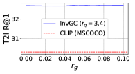
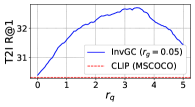
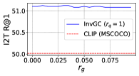
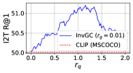
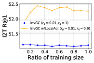
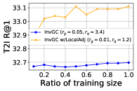
RQ2: Is InvGC (or InvGC w/LocalAdj) sensitive to the hyperparameter and ? To answer the question, we evaluate the R@1 metrics of InvGC with a very large range of hyperparameters respective to the optimal choice adopted. We defer the analysis of InvGC w/LocalAdj to Section C.7. For each task, we fix one of or and tune the other to show the change on the R@1 metrics. The results of the MSCOCO dataset are shown in Figure 2. Although subject to some variation, InvGC constantly outperforms the baseline, which is presented as the red dashed line. This indicates that the proposed method can consistently improve performance with a very large range of parameters.
RQ3: How much data is needed for both proposed methods? Since we use the training query and gallery set as a sampled subset from the hidden distribution of representation, it is quite intuitive to ask if the performance of InvGC or InvGC w/LocalAdj is sensitive to the size of this sampled subset. Therefore, we uniformly sample different ratios of data from both the training query and gallery set at the same time and evaluate the performance of both methods with the identical hyperparameters, as presented in Figure 3. From the results, we conclude that both proposed methods perform stably and robustly regardless of the size of the training data.
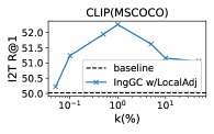
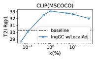
RQ4: Is InvGC w/LocalAdj sensitive to the hyperparameter ? To address the question, we evaluate the R@1 metrics of InvGC w/LocalAdj with a very large range of possible values (even in logarithmic scale) compared to the optimal choice adopted(i.e.,). For each task, we fix everything except the value.The results of MSCOCO dataset are shown in Figure 4. Compared with the baseline, it is safe to claim that the proposed InvGC w/LocalAdj is very robust to the choice of .
4.4 Quantative results
In this section, we present the quantitative results of four cross-modal retrieval benchmarks. Across eight different benchmarks, InvGC and InvGC w/LocalAdj significantly improve upon the baselines, demonstrating the superiority of our proposed methods.
| Normalization | Text-to-Image Retrieval | |||||
|---|---|---|---|---|---|---|
| R@1 | R@5 | R@10 | MdR | MnR | ||
| CLIP | 30.34 | 54.74 | 66.08 | 4.0 | 25.39 | |
| +AvgPool(ratio=0.1) | 30.37 | 54.77 | 66.14 | 4.0 | \ul25.36 | |
| +AvgPool(ratio=0.25) | 30.37 | 54.77 | 66.14 | 4.0 | \ul25.36 | |
| +AvgPool(ratio=0.5) | 30.38 | 54.77 | 66.10 | 4.0 | 25.38 | |
| +AvgPool(ratio=1) | 30.39 | 54.77 | 66.11 | 4.0 | 25.38 | |
| +InvGC | \ul32.70 | \ul57.53 | 68.24 | 4.0 | 24.35 | |
| +InvGC w/LocalAdj | 33.11 | 57.49 | \ul68.19 | 4.0 | 28.95 | |
| Oscar | 52.50 | 80.03 | 87.96 | 1.0 | \ul10.68 | |
| +AvgPool(ratio=0.1) | 52.52 | \ul80.04 | \ul87.95 | 1.0 | 10.70 | |
| +AvgPool(ratio=0.25) | 52.52 | 80.03 | 87.96 | 1.0 | \ul10.68 | |
| +AvgPool(ratio=0.5) | 52.51 | 80.00 | 87.96 | 1.0 | 10.67 | |
| +AvgPool(ratio=1) | 52.50 | 80.02 | 87.96 | 1.0 | \ul10.68 | |
| +InvGC | \ul52.63 | 80.05 | 87.96 | 1.0 | 10.72 | |
| +InvGC w/LocalAdj | 52.93 | 80.05 | 87.78 | 1.0 | 11.09 | |
| Normalization | Text-to-Image Retrieval | |||||
|---|---|---|---|---|---|---|
| R@1 | R@5 | R@10 | MdR | MnR | ||
| CLIP | 58.98 | 83.48 | 90.14 | 1.0 | 6.04 | |
| +AvgPool(ratio=0.1) | 59.10 | 83.56 | \ul90.18 | 1.0 | 6.04 | |
| +AvgPool(ratio=0.25) | 59.10 | 83.56 | \ul90.18 | 1.0 | 6.04 | |
| +AvgPool(ratio=0.5) | 59.10 | \ul83.54 | \ul90.18 | 1.0 | 6.05 | |
| +AvgPool(ratio=1) | 59.10 | \ul83.54 | \ul90.18 | 1.0 | 6.04 | |
| +InvGC | \ul60.18 | 85.30 | 91.20 | 1.0 | 5.52 | |
| +InvGC w/LocalAdj | 60.48 | 85.30 | 91.10 | 1.0 | \ul5.59 | |
| Oscar | 71.60 | 91.50 | 94.96 | 1.0 | 4.24 | |
| +AvgPool(ratio=0.1) | 71.62 | 91.44 | 94.92 | 1.0 | \ul4.25 | |
| +AvgPool(ratio=0.25) | 71.66 | 91.50 | 94.94 | 1.0 | 4.24 | |
| +AvgPool(ratio=0.5) | 71.66 | 91.50 | 94.92 | 1.0 | 4.24 | |
| +AvgPool(ratio=1) | 71.62 | \ul91.52 | 94.96 | 1.0 | 4.24 | |
| +InvGC | \ul71.68 | 91.46 | 95.06 | 1.0 | \ul4.25 | |
| +InvGC w/LocalAdj | 71.74 | 91.56 | \ul94.98 | 1.0 | 4.29 | |
| Normalization | Text-to-Video Retrieval | |||||
|---|---|---|---|---|---|---|
| R@1 | R@5 | R@10 | MdR | MnR | ||
| CLIP4Clip | 44.10 | \ul71.70 | 81.40 | 2.0 | \ul15.51 | |
| +AvgPool(ratio=0.1) | \ul44.20 | 71.60 | \ul81.50 | 2.0 | 15.55 | |
| +AvgPool(ratio=0.25) | \ul44.20 | 71.60 | \ul81.50 | 2.0 | 15.55 | |
| +AvgPool(ratio=0.5) | \ul44.20 | 71.50 | \ul81.50 | 2.0 | 15.54 | |
| +AvgPool(ratio=1) | 44.10 | 71.60 | \ul81.50 | 2.0 | 15.52 | |
| +InvGC | 44.40 | 71.90 | 81.60 | 2.0 | 15.36 | |
| +InvGC w/LocalAdj | 44.40 | \ul71.70 | 81.20 | 2.0 | 15.65 | |
| CLIP2Video | 46.00 | 71.60 | \ul81.60 | 2.0 | 14.51 | |
| +AvgPool(ratio=0.1) | 45.90 | 71.70 | 81.50 | 2.0 | 14.52 | |
| +AvgPool(ratio=0.25) | 46.10 | \ul71.80 | 81.50 | 2.0 | 14.53 | |
| +AvgPool(ratio=0.5) | 46.00 | 71.70 | 81.50 | 2.0 | 14.53 | |
| +AvgPool(ratio=1) | 45.90 | 71.70 | 81.50 | 2.0 | 14.52 | |
| +InvGC | \ul46.20 | 71.70 | 81.30 | 2.0 | 14.44 | |
| +InvGC w/LocalAdj | 46.60 | 72.10 | 81.70 | 2.0 | \ul14.50 | |
| X-CLIP | 46.30 | \ul74.00 | \ul83.40 | 2.0 | 12.80 | |
| +AvgPool(ratio=0.1) | 46.50 | \ul74.00 | \ul83.40 | 2.0 | 12.88 | |
| +AvgPool(ratio=0.25) | 46.40 | \ul74.00 | 83.50 | 2.0 | 12.85 | |
| +AvgPool(ratio=0.5) | 46.30 | \ul74.00 | 83.30 | 2.0 | \ul12.83 | |
| +AvgPool(ratio=1) | 46.20 | \ul74.00 | \ul83.40 | 2.0 | \ul12.83 | |
| +InvGC | 47.30 | \ul74.00 | 83.30 | 2.0 | 13.42 | |
| +InvGC w/LocalAdj | \ul47.10 | 74.20 | 83.50 | 2.0 | 13.09 | |
| Normalization | Text-to-Video Retrieval | |||||
|---|---|---|---|---|---|---|
| R@1 | R@5 | R@10 | MdR | MnR | ||
| CLIP4Clip | 41.85 | 74.44 | 84.84 | 2.0 | \ul6.84 | |
| +AvgPool(ratio=0.1) | 41.83 | \ul74.47 | 84.84 | 2.0 | \ul6.84 | |
| +AvgPool(ratio=0.25) | 41.80 | 74.44 | 84.84 | 2.0 | \ul6.84 | |
| +AvgPool(ratio=0.5) | 41.85 | 74.44 | 84.84 | 2.0 | \ul6.84 | |
| +AvgPool(ratio=1) | 41.88 | 74.44 | 84.84 | 2.0 | \ul6.84 | |
| +InvGC | \ul41.90 | 74.40 | \ul84.86 | 2.0 | \ul6.84 | |
| +InvGC w/LocalAdj | 43.23 | 75.58 | 85.74 | 2.0 | 6.82 | |
| X-CLIP | 46.25 | \ul76.02 | 86.05 | 2.0 | \ul6.37 | |
| +AvgPool(ratio=0.1) | \ul46.47 | 75.94 | 86.05 | 2.0 | 6.38 | |
| +AvgPool(ratio=0.25) | 46.38 | 75.98 | 86.01 | 2.0 | 6.38 | |
| +AvgPool(ratio=0.5) | \ul46.47 | 75.94 | 86.01 | 2.0 | 6.38 | |
| +AvgPool(ratio=1) | 46.43 | 75.89 | 86.01 | 2.0 | 6.38 | |
| +InvGC | 46.43 | 75.68 | \ul86.22 | 2.0 | 6.35 | |
| +InvGC w/LocalAdj | 47.82 | 76.46 | 86.36 | 2.0 | 6.91 | |
| Normalization | Text-to-Video Retrieval | |||||
|---|---|---|---|---|---|---|
| R@1 | R@5 | R@10 | MdR | MnR | ||
| CLIP4Clip | 44.64 | 74.66 | 83.99 | 2.0 | \ul10.32 | |
| +AvgPool(ratio=0.1) | 44.87 | 73.89 | 83.07 | 2.0 | 11.93 | |
| +AvgPool(ratio=0.25) | 45.06 | 74.04 | 83.49 | 2.0 | 11.29 | |
| +AvgPool(ratio=0.5) | 45.12 | 74.32 | 83.66 | 2.0 | 10.76 | |
| +AvgPool(ratio=1) | 45.09 | 74.54 | 83.91 | 2.0 | 10.45 | |
| +InvGC | \ul45.43 | \ul74.82 | \ul84.00 | 2.0 | 10.42 | |
| +InvGC w/LocalAdj | 45.73 | 75.53 | 84.37 | 2.0 | 10.42 | |
| CLIP2Video | 47.05 | 76.97 | 85.59 | 2.0 | \ul9.53 | |
| +AvgPool(ratio=0.1) | 47.04 | 76.98 | 85.61 | 2.0 | 9.54 | |
| +AvgPool(ratio=0.25) | 47.07 | 76.98 | 85.61 | 2.0 | 9.54 | |
| +AvgPool(ratio=0.5) | 47.06 | 76.98 | 85.62 | 2.0 | \ul9.53 | |
| +AvgPool(ratio=1) | 47.06 | 76.97 | 85.61 | 2.0 | \ul9.53 | |
| +InvGC | \ul47.09 | \ul77.00 | \ul85.64 | 2.0 | 9.48 | |
| +InvGC w/LocalAdj | 47.47 | 77.46 | 85.84 | 2.0 | \ul9.53 | |
| X-CLIP | 46.31 | 76.84 | \ul85.31 | 2.0 | 9.59 | |
| +AvgPool(ratio=0.1) | 46.36 | 76.70 | 85.28 | 2.0 | 9.66 | |
| +AvgPool(ratio=0.25) | 46.33 | 76.71 | 85.28 | 2.0 | 9.64 | |
| +AvgPool(ratio=0.5) | 46.35 | 76.71 | 85.25 | 2.0 | 9.62 | |
| +AvgPool(ratio=1) | 46.41 | 76.77 | 85.27 | 2.0 | \ul9.60 | |
| +InvGC | 46.82 | 76.69 | 85.38 | 2.0 | 9.63 | |
| +InvGC w/LocalAdj | \ul46.49 | \ul76.82 | 85.29 | 2.0 | 9.63 | |
| Method | Normalization | Text-to-Audio Retrieval | ||||
|---|---|---|---|---|---|---|
| R@1 | R@5 | R@10 | MdR | MnR | ||
| MoEE* | 6.00 | 20.80 | 32.30 | 23.0 | 60.20 | |
| MMT* | 6.50 | 21.60 | 66.90 | 23.0 | 67.70 | |
| AR-CE | 6.27 | 22.32 | 33.30 | 23.0 | 58.96 | |
| +AvgPool(ratio=0.1) | 6.37 | \ul22.33 | 33.59 | 23.0 | 65.57 | |
| +AvgPool(ratio=0.25) | 6.47 | 22.12 | 33.58 | \ul22.0 | 59.84 | |
| +AvgPool(ratio=0.5) | 6.39 | 22.24 | 33.30 | \ul22.0 | 59.14 | |
| +AvgPool(ratio=1) | 6.28 | 22.32 | 33.30 | 23.0 | \ul58.95 | |
| +InvGC | 6.81 | 22.14 | 34.72 | 21.0 | 61.98 | |
| +InvGC w/LocalAdj | \ul6.58 | 22.35 | \ul34.64 | \ul22.0 | 58.51 | |
| Method | Normalization | Text-to-Audio Retrieval | ||||
|---|---|---|---|---|---|---|
| R@1 | R@5 | R@10 | MdR | MnR | ||
| MoEE* | 23.00 | 55.70 | 71.00 | 4.0 | 16.30 | |
| MMT* | 36.10 | 72.00 | 84.50 | 2.3 | 7.50 | |
| AR-CE | \ul22.33 | \ul54.49 | \ul70.54 | \ul5.0 | 15.89 | |
| +AvgPool(ratio=0.1) | \ul22.33 | \ul54.49 | \ul70.54 | \ul5.0 | 15.89 | |
| +AvgPool(ratio=0.25) | \ul22.33 | \ul54.49 | \ul70.54 | \ul5.0 | 15.89 | |
| +AvgPool(ratio=0.5) | \ul22.33 | \ul54.49 | \ul70.54 | \ul5.0 | 15.89 | |
| +AvgPool(ratio=1) | \ul22.33 | \ul54.49 | \ul70.54 | \ul5.0 | 15.89 | |
| +InvGC | \ul22.33 | 54.46 | 70.56 | \ul5.0 | 15.89 | |
| +InvGC w/LocalAdj | 24.07 | 55.69 | 70.20 | 4.0 | \ul16.54 | |
Text-Image Retrieval. Results are presented in Tables 3 and 4. We observe that one of our methods achieves the best performance on R@1, R@5, and R@10 by a large margin. When evaluated on the CLIP method, InvGC w/LocalAdj outperforms the baselines on both the MSCOCO and Flickr30k datasets, improving R@1 and R@5 by at least 2% compared to all baselines.
Text-Video Retrieval. Results are presented in Tables 5, 6 and 7. We can also conclude that one of our methods achieves the best performance on R@1, R@5, and R@10. Specifically, on the ActivityNet dataset, InvGC w/LocalAdj shows excellent performance with both CLIP4CLIP and X-CLIP methods, significantly outperforming all the baselines on R@1 and R@5 roughly by 2%.
Text-Audio Retrieval. Results are presented in Tables 8 and 9. On the CLOTHO dataset, InvGC exhibits significantly better performance compared to all the baselines while InvGC w/LocalAdj achieves the best results on the AudioCaps dataset.
In summary, our experiments demonstrate that employing InvGC consistently improves retrieval performance across different datasets and retrieval tasks. The models with InvGC demonstrate better accuracy and ranking in retrieving relevant videos, images, and textual descriptions based on given queries. The complete results of retrieval performance can be found in Section C.6.
5 Conclusion
This paper addressed representation degeneration problem in cross-modal retrieval, which led to a decrease in retrieval performance. The representation degeneration problem was validated across multiple benchmarks and methods. To alleviate this issue, we proposed a novel method called InvGC, inspired by graph convolution and average pooling. The method established a graph topology structure within the datasets and applied graph convolution in an inverse form with subtraction over the neighborhood. Additionally, we designed the adjacency matrix, LocalAdj, that only leveraged the nearest neighbors of each data point rather than the entire dataset, resulting in a more effective and efficient method, InvGC w/LocalAdj. Both InvGC and InvGC w/LocalAdj were validated through theoretical analysis and demonstrated their ability to separate representations. Finally, extensive experiments on various cross-modal benchmarks showed that both of our methods successfully alleviated the problem of representation degeneration and, as a result, improved retrieval performance.
Limitations
First, although InvGC has been validated through theoretical analysis and demonstrated its efficacy in separating representations, its performance may vary across different datasets and modalities. The effectiveness of our method might be influenced by variations in dataset characteristics, such as data distribution, scale, and complexity. Further investigation and experimentation on a wider range of datasets are needed to fully understand the generalizability of InvGC and its performance under diverse conditions.
Second, while our method shows promising results in alleviating the representation degeneration problem, it is worth noting that cross-modal retrieval tasks can still pose challenges due to inherent differences in modalities. Variations in feature spaces, data modalities, and semantic gaps between modalities may limit the overall retrieval performance. Future research efforts should focus on exploring complementary techniques, such as multimodal fusion, attention mechanisms, or domain adaptation, to further enhance the retrieval accuracy and alleviate representation degeneration problem.
In the future, it would be interesting to explore the performance of InvGC on diverse datasets, the challenges associated with cross-modal differences, and better definitions or metrics for measuring representation degeneration problem.
References
- Baranwal et al. (2023) Aseem Baranwal, Kimon Fountoulakis, and Aukosh Jagannath. 2023. Effects of graph convolutions in multi-layer networks. In The Eleventh International Conference on Learning Representations.
- Bellman (2015) Richard Bellman. 2015. Adaptive Control Processes - A Guided Tour (Reprint from 1961), volume 2045 of Princeton Legacy Library. Princeton University Press.
- Bogolin et al. (2022) Simion-Vlad Bogolin, Ioana Croitoru, Hailin Jin, Yang Liu, and Samuel Albanie. 2022. Cross modal retrieval with querybank normalisation. In IEEE/CVF Conference on Computer Vision and Pattern Recognition, CVPR 2022, New Orleans, LA, USA, June 18-24, 2022, pages 5184–5195. IEEE.
- Boureau et al. (2010) Y-Lan Boureau, Jean Ponce, and Yann LeCun. 2010. A theoretical analysis of feature pooling in visual recognition. In Proceedings of the 27th International Conference on International Conference on Machine Learning, ICML’10, page 111–118, Madison, WI, USA. Omnipress.
- Bruna et al. (2014) Joan Bruna, Wojciech Zaremba, Arthur Szlam, and Yann LeCun. 2014. Spectral networks and locally connected networks on graphs.
- Chen and Dolan (2011) David Chen and William Dolan. 2011. Collecting highly parallel data for paraphrase evaluation. In Proceedings of the 49th Annual Meeting of the Association for Computational Linguistics: Human Language Technologies, pages 190–200, Portland, Oregon, USA. Association for Computational Linguistics.
- Chen et al. (2020) Shizhe Chen, Yida Zhao, Qin Jin, and Qi Wu. 2020. Fine-grained video-text retrieval with hierarchical graph reasoning. In 2020 IEEE/CVF Conference on Computer Vision and Pattern Recognition, CVPR 2020, Seattle, WA, USA, June 13-19, 2020, pages 10635–10644. Computer Vision Foundation / IEEE.
- Cheng et al. (2021) Xing Cheng, Hezheng Lin, Xiangyu Wu, Fan Yang, and Dong Shen. 2021. Improving video-text retrieval by multi-stream corpus alignment and dual softmax loss. CoRR, abs/2109.04290.
- Croitoru et al. (2021) Ioana Croitoru, Simion-Vlad Bogolin, Marius Leordeanu, Hailin Jin, Andrew Zisserman, Samuel Albanie, and Yang Liu. 2021. Teachtext: Crossmodal generalized distillation for text-video retrieval. In 2021 IEEE/CVF International Conference on Computer Vision, ICCV 2021, Montreal, QC, Canada, October 10-17, 2021, pages 11563–11573. IEEE.
- de la Pena and Montgomery-Smith (1995) Victor H. de la Pena and S. J. Montgomery-Smith. 1995. Decoupling Inequalities for the Tail Probabilities of Multivariate -Statistics. The Annals of Probability, 23(2):806 – 816.
- Devlin et al. (2019) Jacob Devlin, Ming-Wei Chang, Kenton Lee, and Kristina Toutanova. 2019. BERT: pre-training of deep bidirectional transformers for language understanding. In Proceedings of the 2019 Conference of the North American Chapter of the Association for Computational Linguistics: Human Language Technologies, NAACL-HLT 2019, Minneapolis, MN, USA, June 2-7, 2019, Volume 1 (Long and Short Papers), pages 4171–4186. Association for Computational Linguistics.
- Drossos et al. (2020) Konstantinos Drossos, Samuel Lipping, and Tuomas Virtanen. 2020. Clotho: an Audio Captioning Dataset. In ICASSP 2020 - 2020 IEEE International Conference on Acoustics, Speech and Signal Processing (ICASSP), pages 736–740. ISSN: 2379-190X.
- Fabian Caba Heilbron and Niebles (2015) Bernard Ghanem Fabian Caba Heilbron, Victor Escorcia and Juan Carlos Niebles. 2015. Activitynet: A large-scale video benchmark for human activity understanding. In Proceedings of the IEEE Conference on Computer Vision and Pattern Recognition, pages 961–970.
- Gabeur et al. (2020) Valentin Gabeur, Chen Sun, Karteek Alahari, and Cordelia Schmid. 2020. Multi-modal transformer for video retrieval. In Computer Vision - ECCV 2020 - 16th European Conference, Glasgow, UK, August 23-28, 2020, Proceedings, Part IV, volume 12349 of Lecture Notes in Computer Science, pages 214–229. Springer.
- Gan et al. (2020) Zhe Gan, Yen-Chun Chen, Linjie Li, Chen Zhu, Yu Cheng, and Jingjing Liu. 2020. Large-scale adversarial training for vision-and-language representation learning. In Advances in Neural Information Processing Systems 33: Annual Conference on Neural Information Processing Systems 2020, NeurIPS 2020, December 6-12, 2020, virtual.
- Gao et al. (2019) Jun Gao, Di He, Xu Tan, Tao Qin, Liwei Wang, and Tie-Yan Liu. 2019. Representation degeneration problem in training natural language generation models. In 7th International Conference on Learning Representations, ICLR 2019, New Orleans, LA, USA, May 6-9, 2019. OpenReview.net.
- Gao et al. (2021) Zijian Gao, Jingyu Liu, Sheng Chen, Dedan Chang, Hao Zhang, and Jinwei Yuan. 2021. CLIP2TV: an empirical study on transformer-based methods for video-text retrieval. CoRR, abs/2111.05610.
- Gilmer et al. (2017) Justin Gilmer, Samuel S. Schoenholz, Patrick F. Riley, Oriol Vinyals, and George E. Dahl. 2017. Neural message passing for quantum chemistry. In Proceedings of the 34th International Conference on Machine Learning - Volume 70, ICML’17, page 1263–1272. JMLR.org.
- Gong et al. (2013) Yunchao Gong, Svetlana Lazebnik, Albert Gordo, and Florent Perronnin. 2013. Iterative quantization: A procrustean approach to learning binary codes for large-scale image retrieval. IEEE Trans. Pattern Anal. Mach. Intell., 35(12):2916–2929.
- Goodfellow et al. (2016) Ian Goodfellow, Yoshua Bengio, and Aaron Courville. 2016. Deep Learning. MIT Press. http://www.deeplearningbook.org.
- Gorti et al. (2022) Satya Krishna Gorti, Noël Vouitsis, Junwei Ma, Keyvan Golestan, Maksims Volkovs, Animesh Garg, and Guangwei Yu. 2022. X-pool: Cross-modal language-video attention for text-video retrieval. In IEEE/CVF Conference on Computer Vision and Pattern Recognition, CVPR 2022, New Orleans, LA, USA, June 18-24, 2022, pages 4996–5005. IEEE.
- (22) Simple GraphConv. Pyg description of simple graph convolution. https://pytorch-geometric.readthedocs.io/en/latest/generated/torch_geometric.nn.conv.SimpleConv.html#torch_geometric.nn.conv.SimpleConv. Accessed: 2023-06-17.
- Hamilton (2020) William L. Hamilton. 2020. Graph representation learning. Synthesis Lectures on Artificial Intelligence and Machine Learning, 14(3):1–159.
- He et al. (2016) Kaiming He, Xiangyu Zhang, Shaoqing Ren, and Jian Sun. 2016. Deep residual learning for image recognition. In 2016 IEEE Conference on Computer Vision and Pattern Recognition, CVPR 2016, Las Vegas, NV, USA, June 27-30, 2016, pages 770–778. IEEE Computer Society.
- Hendricks et al. (2017) Lisa Anne Hendricks, Oliver Wang, Eli Shechtman, Josef Sivic, Trevor Darrell, and Bryan Russell. 2017. Localizing Moments in Video with Natural Language. In 2017 IEEE International Conference on Computer Vision (ICCV), pages 5804–5813, Venice. IEEE.
- Huang et al. (2021) Zhenyu Huang, Guocheng Niu, Xiao Liu, Wenbiao Ding, Xinyan Xiao, Hua Wu, and Xi Peng. 2021. Learning with noisy correspondence for cross-modal matching. In Advances in Neural Information Processing Systems, volume 34, pages 29406–29419. Curran Associates, Inc.
- Keogh and Mueen (2017) Eamonn Keogh and Abdullah Mueen. 2017. Curse of Dimensionality, pages 314–315. Springer US, Boston, MA.
- Kim et al. (2019) Chris Dongjoo Kim, Byeongchang Kim, Hyunmin Lee, and Gunhee Kim. 2019. AudioCaps: Generating captions for audios in the wild. In Proceedings of the 2019 Conference of the North American Chapter of the Association for Computational Linguistics: Human Language Technologies, Volume 1 (Long and Short Papers), pages 119–132, Minneapolis, Minnesota. Association for Computational Linguistics.
- Kim et al. (2023) Taehoon Kim, Pyunghwan Ahn, Sangyun Kim, Sihaeng Lee, Mark Marsden, Alessandra Sala, Seung Hwan Kim, Bohyung Han, Kyoung Mu Lee, Honglak Lee, Kyounghoon Bae, Xiangyu Wu, Yi Gao, Hailiang Zhang, Yang Yang, Weili Guo, Jianfeng Lu, Youngtaek Oh, Jae Won Cho, Dong jin Kim, In So Kweon, Junmo Kim, Wooyoung Kang, Won Young Jhoo, Byungseok Roh, Jonghwan Mun, Solgil Oh, Kenan Emir Ak, Gwang-Gook Lee, Yan Xu, Mingwei Shen, Kyomin Hwang, Wonsik Shin, Kamin Lee, Wonhark Park, Dongkwan Lee, Nojun Kwak, Yujin Wang, Yimu Wang, Tiancheng Gu, Xingchang Lv, and Mingmao Sun. 2023. Nice: Cvpr 2023 challenge on zero-shot image captioning.
- Kipf and Welling (2017) Thomas N. Kipf and Max Welling. 2017. Semi-supervised classification with graph convolutional networks. In International Conference on Learning Representations.
- Koepke et al. (2022) A. Sophia Koepke, Andreea-Maria Oncescu, Joao Henriques, Zeynep Akata, and Samuel Albanie. 2022. Audio Retrieval with Natural Language Queries: A Benchmark Study. IEEE Transactions on Multimedia, pages 1–1. Conference Name: IEEE Transactions on Multimedia.
- Lei et al. (2021) Jie Lei, Linjie Li, Luowei Zhou, Zhe Gan, Tamara L. Berg, Mohit Bansal, and Jingjing Liu. 2021. Less is more: Clipbert for video-and-language learning via sparse sampling. In IEEE Conference on Computer Vision and Pattern Recognition, CVPR 2021, virtual, June 19-25, 2021, pages 7331–7341. Computer Vision Foundation / IEEE.
- Li et al. (2020) Xiujun Li, Xi Yin, Chunyuan Li, Pengchuan Zhang, Xiaowei Hu, Lei Zhang, Lijuan Wang, Houdong Hu, Li Dong, Furu Wei, Yejin Choi, and Jianfeng Gao. 2020. Oscar: Object-semantics aligned pre-training for vision-language tasks. In Computer Vision - ECCV 2020 - 16th European Conference, Glasgow, UK, August 23-28, 2020, Proceedings, Part XXX, volume 12375 of Lecture Notes in Computer Science, pages 121–137. Springer.
- Liang et al. (2022) Weixin Liang, Yuhui Zhang, Yongchan Kwon, Serena Yeung, and James Zou. 2022. Mind the gap: Understanding the modality gap in multi-modal contrastive representation learning. In Advances in neural information processing systems.
- Lin et al. (2014) Tsung-Yi Lin, Michael Maire, Serge J. Belongie, James Hays, Pietro Perona, Deva Ramanan, Piotr Dollár, and C. Lawrence Zitnick. 2014. Microsoft COCO: common objects in context. In Computer Vision - ECCV 2014 - 13th European Conference, Zurich, Switzerland, September 6-12, 2014, Proceedings, Part V, volume 8693 of Lecture Notes in Computer Science, pages 740–755. Springer.
- Liong et al. (2017) Venice Erin Liong, Jiwen Lu, Yap-Peng Tan, and Jie Zhou. 2017. Cross-modal deep variational hashing. In IEEE International Conference on Computer Vision, ICCV 2017, Venice, Italy, October 22-29, 2017, pages 4097–4105. IEEE Computer Society.
- Liu et al. (2019) Yang Liu, Samuel Albanie, Arsha Nagrani, and Andrew Zisserman. 2019. Use what you have: Video retrieval using representations from collaborative experts. In 30th British Machine Vision Conference 2019, BMVC 2019, Cardiff, UK, September 9-12, 2019, page 279. BMVA Press.
- Luo et al. (2022) Huaishao Luo, Lei Ji, Ming Zhong, Yang Chen, Wen Lei, Nan Duan, and Tianrui Li. 2022. Clip4clip: An empirical study of CLIP for end to end video clip retrieval and captioning. Neurocomputing, 508:293–304.
- Ma et al. (2022) Yiwei Ma, Guohai Xu, Xiaoshuai Sun, Ming Yan, Ji Zhang, and Rongrong Ji. 2022. X-CLIP: end-to-end multi-grained contrastive learning for video-text retrieval. In MM ’22: The 30th ACM International Conference on Multimedia, Lisboa, Portugal, October 10 - 14, 2022, pages 638–647. ACM.
- Micciancio and Voulgaris (2010) Daniele Micciancio and Panagiotis Voulgaris. 2010. Faster exponential time algorithms for the shortest vector problem. In Proceedings of the Twenty-First Annual ACM-SIAM Symposium on Discrete Algorithms, SODA ’10, page 1468–1480, USA. Society for Industrial and Applied Mathematics.
- Miech et al. (2021) Antoine Miech, Jean-Baptiste Alayrac, Ivan Laptev, Josef Sivic, and Andrew Zisserman. 2021. Thinking fast and slow: Efficient text-to-visual retrieval with transformers. In IEEE Conference on Computer Vision and Pattern Recognition, CVPR 2021, virtual, June 19-25, 2021, pages 9826–9836. Computer Vision Foundation / IEEE.
- Miech et al. (2020) Antoine Miech, Ivan Laptev, and Josef Sivic. 2020. Learning a Text-Video Embedding from Incomplete and Heterogeneous Data. ArXiv:1804.02516 [cs].
- Oncescu et al. (2021) Andreea-Maria Oncescu, A. Sophia Koepke, João F. Henriques, Zeynep Akata, and Samuel Albanie. 2021. Audio retrieval with natural language queries. In Interspeech 2021, 22nd Annual Conference of the International Speech Communication Association, Brno, Czechia, 30 August - 3 September 2021, pages 2411–2415. ISCA.
- Park et al. (2022) Jae Sung Park, Sheng Shen, Ali Farhadi, Trevor Darrell, Yejin Choi, and Anna Rohrbach. 2022. Exposing the limits of video-text models through contrast sets. In Proceedings of the 2022 Conference of the North American Chapter of the Association for Computational Linguistics: Human Language Technologies, pages 3574–3586, Seattle, United States. Association for Computational Linguistics.
- Plummer et al. (2017) Bryan A. Plummer, Liwei Wang, Chris M. Cervantes, Juan C. Caicedo, Julia Hockenmaier, and Svetlana Lazebnik. 2017. Flickr30k entities: Collecting region-to-phrase correspondences for richer image-to-sentence models. Int. J. Comput. Vis., 123(1):74–93.
- Radford et al. (2021) Alec Radford, Jong Wook Kim, Chris Hallacy, Aditya Ramesh, Gabriel Goh, Sandhini Agarwal, Girish Sastry, Amanda Askell, Pamela Mishkin, Jack Clark, Gretchen Krueger, and Ilya Sutskever. 2021. Learning transferable visual models from natural language supervision. In Proceedings of the 38th International Conference on Machine Learning, ICML 2021, 18-24 July 2021, Virtual Event, volume 139 of Proceedings of Machine Learning Research, pages 8748–8763. PMLR.
- Radovanovic et al. (2010) Milos Radovanovic, Alexandros Nanopoulos, and Mirjana Ivanovi. 2010. Hubs in space: Popular nearest neighbors in high-dimensional data. Journal of Machine Learning Research, 11(86):2487–2531.
- Singh et al. (2022) Amanpreet Singh, Ronghang Hu, Vedanuj Goswami, Guillaume Couairon, Wojciech Galuba, Marcus Rohrbach, and Douwe Kiela. 2022. FLAVA: A foundational language and vision alignment model. In IEEE/CVF Conference on Computer Vision and Pattern Recognition, CVPR 2022, New Orleans, LA, USA, June 18-24, 2022, pages 15617–15629. IEEE.
- Su et al. (2019) Shupeng Su, Zhisheng Zhong, and Chao Zhang. 2019. Deep joint-semantics reconstructing hashing for large-scale unsupervised cross-modal retrieval. In 2019 IEEE/CVF International Conference on Computer Vision, ICCV 2019, Seoul, Korea (South), October 27 - November 2, 2019, pages 3027–3035. IEEE.
- Velickovic et al. (2018) Petar Velickovic, Guillem Cucurull, Arantxa Casanova, Adriana Romero, Pietro Lio, and Yoshua Bengio. 2018. Graph attention networks. In International Conference on Learning Representations.
- Wang et al. (2022a) Haoran Wang, Di Xu, Dongliang He, Fu Li, Zhong Ji, Jungong Han, and Errui Ding. 2022a. Boosting video-text retrieval with explicit high-level semantics. In MM ’22: The 30th ACM International Conference on Multimedia, Lisboa, Portugal, October 10 - 14, 2022, pages 4887–4898. ACM.
- Wang et al. (2022b) Xiaohan Wang, Linchao Zhu, Zhedong Zheng, Mingliang Xu, and Yi Yang. 2022b. Align and tell: Boosting text-video retrieval with local alignment and fine-grained supervision. IEEE Transactions on Multimedia, pages 1–11.
- Wang et al. (2023) Yimu Wang, Xiangru Jian, and Bo Xue. 2023. Balance act: Mitigating hubness in cross-modal retrieval with query and gallery banks.
- Wang et al. (2020a) Yimu Wang, Shiyin Lu, and Lijun Zhang. 2020a. Searching privately by imperceptible lying: A novel private hashing method with differential privacy. In Proceedings of the 28th ACM International Conference on Multimedia, page 2700–2709.
- Wang and Shi (2023) Yimu Wang and Peng Shi. 2023. Video-Text Retrieval by Supervised Multi-Space Multi-Grained Alignment. ArXiv:2302.09473 [cs].
- Wang et al. (2020b) Yimu Wang, Xiu-Shen Wei, Bo Xue, and Lijun Zhang. 2020b. Piecewise hashing: A deep hashing method for large-scale fine-grained search. In Pattern Recognition and Computer Vision - Third Chinese Conference, PRCV 2020, Nanjing, China, October 16-18, 2020, Proceedings, Part II, pages 432–444.
- Wang et al. (2021) Yimu Wang, Bo Xue, Quan Cheng, Yuhui Chen, and Lijun Zhang. 2021. Deep unified cross-modality hashing by pairwise data alignment. In Proceedings of the Thirtieth International Joint Conference on Artificial Intelligence, IJCAI-21, pages 1129–1135.
- Xu et al. (2016) Jun Xu, Tao Mei, Ting Yao, and Yong Rui. 2016. MSR-VTT: A large video description dataset for bridging video and language. In 2016 IEEE Conference on Computer Vision and Pattern Recognition, CVPR 2016, Las Vegas, NV, USA, June 27-30, 2016, pages 5288–5296. IEEE Computer Society.
- Yang et al. (2022) Mouxing Yang, Zhenyu Huang, Peng Hu, Taihao Li, Jiancheng Lv, and Xi Peng. 2022. Learning with twin noisy labels for visible-infrared person re-identification. In 2022 IEEE/CVF Conference on Computer Vision and Pattern Recognition (CVPR), pages 14288–14297.
- Yu et al. (2023) Qiying Yu, Yang Liu, Yimu Wang, Ke Xu, and Jingjing Liu. 2023. Multimodal federated learning via contrastive representation ensemble. In The Eleventh International Conference on Learning Representations.
- Yu et al. (2022) Sangwon Yu, Jongyoon Song, Heeseung Kim, Seongmin Lee, Woo-Jong Ryu, and Sungroh Yoon. 2022. Rare tokens degenerate all tokens: Improving neural text generation via adaptive gradient gating for rare token embeddings. In Proceedings of the 60th Annual Meeting of the Association for Computational Linguistics (Volume 1: Long Papers), pages 29–45, Dublin, Ireland. Association for Computational Linguistics.
- Zhang et al. (2020) Zhong Zhang, Chongming Gao, Cong Xu, Rui Miao, Qinli Yang, and Junming Shao. 2020. Revisiting representation degeneration problem in language modeling. In Findings of the Association for Computational Linguistics: EMNLP 2020, pages 518–527, Online. Association for Computational Linguistics.
- Zhao et al. (2022) Shuai Zhao, Linchao Zhu, Xiaohan Wang, and Yi Yang. 2022. Centerclip: Token clustering for efficient text-video retrieval. In Proceedings of the 45th International ACM SIGIR Conference on Research and Development in Information Retrieval, SIGIR ’22, page 970–981, New York, NY, USA. Association for Computing Machinery.
- Zhong et al. (2017) Zhun Zhong, Liang Zheng, Donglin Cao, and Shaozi Li. 2017. Re-ranking person re-identification with k-reciprocal encoding. In 2017 IEEE Conference on Computer Vision and Pattern Recognition, CVPR 2017, Honolulu, HI, USA, July 21-26, 2017, pages 3652–3661. IEEE Computer Society.
\ul
Appendix A Related Work
We review prior work in cross-modal retrieval and representation degeneration, which are the two most related areas to our work.
Cross-modal Retrival. The goal of cross-modal retrieval is to learn a common representation space, where the similarity between samples from different modalities can be directly measured. Recently, inspired by the success of deep learning Devlin et al. (2019); He et al. (2016), numerous methods based on deep neural networks have been proposed for image-text retrieval Radford et al. (2021), video-text retrieval Luo et al. (2022), and audio-text retrieval Oncescu et al. (2021). Further, to learn a better representation space, vision-language pretraining Gan et al. (2020); Li et al. (2020); Singh et al. (2022) on large-scale unlabeled cross-modal data has been widely employed and have shown promising performance. Motivated by this, recent works have attempted to pretrain or fine-tune cross-modal retrieval models, e.g., image-text retrieval Radford et al. (2021); Li et al. (2020), video-text retrieval Chen et al. (2020); Cheng et al. (2021); Gao et al. (2021); Gorti et al. (2022); Lei et al. (2021); Ma et al. (2022); Park et al. (2022); Wang et al. (2022a, b); Zhao et al. (2022), and audio-text retrieval Oncescu et al. (2021) in an end-to-end manner.
In contrast to the methods that focus on improving the representation learning ability, another line of cross-modal retrieval research has focused on improving the effectiveness of retrieval, including k-d trees Bellman (2015), re-ranking Zhong et al. (2017); Miech et al. (2021), query expansion Chen et al. (2020), vector compression schemes based on binary codes Su et al. (2019); Liong et al. (2017) and quantization Gong et al. (2013) that help address the curse of dimensionality Keogh and Mueen (2017). However, a recent study Liang et al. (2022) shows that the representation degeneration problem has significantly affected the performance of multi-modal learning. To investigate the influence of representation degeneration problem in the cross-modal retrieval,
we show that representation degeneration problem widely exists in different datasets and models.
Representation degeneration. The representation degeneration problem was first introduced in the natural language processing (NLP) area Gao et al. (2019). It was found that when training a model for natural language generation tasks through likelihood maximization with the weight-tying trick, especially with large training datasets, many of the learned word embeddings tend to degenerate and be distributed into a narrow cone. This limitation largely reduces the representation power of word embeddings. The representation degeneration problem leads to an increase in the overall similarity between token embeddings, which has a negative effect on the performance of the models. It was noted that Laplacian regularization can address this problem better than cosine regularization through theoretical proof and empirical experiments Zhang et al. (2020). Subsequent work highlighted Yu et al. (2022) that the training dynamics of the token embeddings focus on rare token embedding which leads to the degeneration problem for all tokens. To this end, they use adaptive gradient gating which gates the specific part of the gradient for rare token embeddings and thus better alleviates the data degeneration problem.
Though representation degeneration has been explored in NLP, it remains unexplored in multi-modal learning for a long time. A recent work Liang et al. (2022) shows that the representation generated by a common deep neural network is restricted to a narrow cone and consequently, with two modality-dependent encoders, the representations from the two modalities are clearly apart during the whole training procedure. Further, they also show that varying the modality gap distance has a significant impact on improving the model’s downstream zero-shot classification performance and fairness.
To step forward towards better representation learning in cross-modal retrieval, different from the previous methods in NLP which focus on addressing this problem in the training procedure, we propose a novel method, namely InvGC, which proposes to avoid representation degeneration in a post-processing manner.
Inspired by the representation aggregation induced by graph convolution Keogh and Mueen (2017); Baranwal et al. (2023), we utilize the graph convolution in an opposite way to separate the data points that share similar representation.
As the first method in solving the representation degeneration problem in cross-modal retrieval, InvGC does not require retraining the model or any other time-consuming operation. InvGC achieves better retrieval performance with a larger margin between different representations compared to the baselines and does this faster.
Appendix B Elaborations on Methodologies
B.1 Graph Convolution
Graph convolution is a mathematical operation that transforms the features of nodes in a graph based on their local neighborhoods. The objective is to learn a function of signals/features on a graph, which takes into account the graph structure and the node features. It can be regarded as a generalization of convolutions to non-Euclidean data Bruna et al. (2014). The operation is first introduced and popularized in the work of Graph Convolution Networks Kipf and Welling (2017), which is considered one of the most seminal papers in the area of graph learning.
The main idea behind a graph convolution operation is to generate a new representation for each node that captures the local neighborhood information around it. This is usually achieved by aggregating feature information from a node’s direct neighbors, sometimes including the node itself. Formally, it can be defined as a special case of a Message Passing Network (MPNN), in which vector messages are exchanged between nodes and updated using neural networks Gilmer et al. (2017). The basic operation of MPNN can be expressed as Hamilton (2020)
where (short for update) and (short for aggregation) are arbitrary differentiable functions (i.e., neural networks) and is the embedding(representation) of node at -th iteration. is the "message" that is aggregated from ’s graph neighborhood .
In this study, we adopt a simple message passing operator that performs non-trainable propagation since we want to propose a post-processing method with any training. The adopt operator is actually the backbone of multiple GNN studies, which can be expressed as GraphConv ,
where defines a custom aggregation scheme. is updated representation of node and is edge weight between node and .
For the sake of simplicity and explainability, we concretize the above operation only with simple addition and self-loop, as follows,
| (10) |
Note that the only difference with Equation 10 and inverse convolution Equation 3 we apply in the study is that addiction is replaced with subtraction, leading to the name ’inverse’.
B.2 Average Pooling in CNN
Average pooling is one type of pooling layers that conducts dimensionality reduction, reducing the number of parameters in the input Goodfellow et al. (2016). Similar to the convolutional layer, the pooling operation sweeps a filter across the entire input, but the difference is that this filter does not have any weights. Instead, the kernel applies an aggregation function to the values within the receptive field. Specifically, the adopted average pooling calculates the average value within the receptive field of the filter as it moves across the input. Here in this study, the receptive field is subject to the size of the neighborhood of each data point.
B.3 Distribution of Data Representation
While we keep using the discrete gallery and query set like in Equation 3, they can be regarded as sampled results from the hidden continuous distribution dependent on the intrinsic properties of the corresponding dataset and the representation learning method applied. Therefore, ideally, two gallery sets sampled from the same dataset will probably have different scores even with the same representation learning method due to the variance introduced by the sampling process. That is to say, performing the same inverse convolution operation on the two sampled gallery sets might have quite different effects, especially when the sample size is small. Also, since the proposed method in this study is a post-processing approach without any training, we need to control the magnitude of the convolution with the help of some hyperparameters. The reason for doing this is to control the change in the representation of the gallery data that has already been aligned with the embedding space of query data by the representation learning model. Given the sampled gallery set is small, this means a very large variance in the value of the best hyperparameters as well.
Unfortunately, it is quite common in practice that we only have a small sampled gallery set. Usually, when cross-modal retrieval is carried out, we constantly cut down the size of the gallery set with the help of some pre-ranking or indexing techniques. This process can be somehow regarded as sampling a set from the distribution that is empirically represented by the whole gallery set. Also, during the evaluation of any method on various datasets, the size of the test or evaluation gallery set is typically much smaller compared to the training set.
Both cases make the result of the proposed methods subjected to potentially large variance.
However, it would be more promising that our method is generally stable and robust to any size of the gallery set. The ideal case would be that we can perform the inverse convolution similar to Equation 1 but based on the continuous distribution, where is data point to be sampled from the hidden distribution, as follows,
| (11) |
However, it is impossible to have exact access to this hidden distribution in practice. The best approximation is the training (or validation) gallery set since it is the largest one we can obtain. Therefore, we can perform the inverse convolution on . Note that the distribution of the query set should theoretically be similar to that of as this a basic assumption in machine learning Bogolin et al. (2022). Therefore, it is possible to combine the (train or validation) gallery set and the (train or validation) query set to be the even better estimation of the hidden distribution. Thus, we go on to refine InvGC as in Equation 4,
In general, with reasonable and general assumptions, we strike the importance of utilizing the data of both the modality from the training set when we want to capture a more accurate and stable distribution of data representation. The idea is not bound to the proposed methods and can be adopted by any future work on the post-processing of cross-modal retrieval tasks.
Appendix C Experiments
C.1 Datasets Details
The experiments are conducted on eight cross-modal benchmarks, which include four video-text retrieval benchmarks (MSR-VTT Xu et al. (2016), MSVD Chen and Dolan (2011), ActivityNet Fabian Caba Heilbron and Niebles (2015), and DiDemo Hendricks et al. (2017)), two image-text retrieval benchmarks (MSCOCO Lin et al. (2014) and Flickr30k Plummer et al. (2017)), as well as two audio-text retrieval benchmarks (AudioCaps Kim et al. (2019) and CLOTHO Drossos et al. (2020)). The details of the datasets are presented below:
-
•
MSR-VTT Xu et al. (2016): Comprises approximately 10k videos, each accompanied by 20 captions. For text-video retrieval, we follow the protocol set by previous works Liu et al. (2019); Croitoru et al. (2021); Luo et al. (2022); Ma et al. (2022); Park et al. (2022), using both the official (full) split and the 1k-A split. The full split includes 2,990 videos for testing and 497 for validation, whereas the 1k-A split has 1,000 videos for testing and around 9,000 for training.
-
•
MSVD Chen and Dolan (2011): Contains 1,970 videos and about 80k captions. The standard split used in prior works Liu et al. (2019); Croitoru et al. (2021); Luo et al. (2022); Park et al. (2022) is adopted for reporting results, which includes 1,200 videos for training, 100 for validation, and 670 for testing.
-
•
ActivityNet Fabian Caba Heilbron and Niebles (2015): Contains 20k videos and approximately 100K descriptive sentences. These videos are extracted from YouTube. We employ a paragraph video retrieval setup as defined in prior works Liu et al. (2019); Croitoru et al. (2021); Luo et al. (2022); Park et al. (2022). We report results on the val1 split. The training split includes 10,009 videos, with 4,917 videos allocated for testing.
-
•
DiDemo Hendricks et al. (2017): Includes over 10,000 personal videos, each lasting between 25-30 seconds, along with over 40,000 localized text descriptions. The videos are divided into training (8,395), validation (1,065), and testing (1,004) sets.
-
•
MSCOCO Lin et al. (2014): Consists of 123k images, each accompanied by 5 captions. The 5k split is used for evaluation.
-
•
Flickr30k Plummer et al. (2017): This dataset contains 31,000 images collected from Flickr, each accompanied by 5 reference sentences provided by human annotators.
- •
-
•
CLOTHO Drossos et al. (2020): Comprises of 4,981 audio samples of 15 to 30 seconds in duration and 24,905 captions of eight to 20 words in length (five captions for each audio sample).
C.2 Experiment Details
The public codes and weights of all the tasks in this study are summarized in Table 10. Note that there is no available trained model for CLIP and X-CLIP. Therefore, we train both models on a single A100 GPU with the hyperparameters recommended by the original studies.
C.3 Prevalence of Representation Degeneration Problem across Datasets and Methods
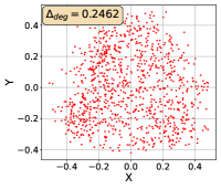
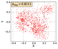
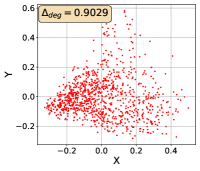
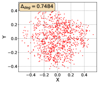
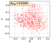
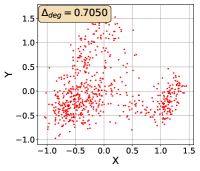
To show that the representation degeneration problem prevails in all datasets, methods, and tasks, we perform the same analysis in Figure 1(a). We uniformly sample a subset of the gallery set of both retrieval tasks (i.e., text to other modality or other modality to text, other modalities can be video, image, or audio depending on the dataset), and perform PCA upon it to reduce the dimension of the representations down to 2, which is the first two principal dimensions. The results are presented in Figure 5. Note that (i.e., the degree of representation degeneration problem) included in each figure is the one for the complete gallery set instead of the sampled set used in the figure.
For this qualitative but very intuitive study, We firmly validate again that almost all the data representations gathered in a very narrow cone in the embedding space for basically all the datasets, methods, and tasks. Also, though subject to the difference between datasets and methods, we can witness that a more convex-shaped distribution usually generally leads to a larger .
The results imply the universality of the representation degeneration problem. More quantitative results can be found in RQ1 in Section 4.3 and in the Continuation on RQ1 section (Section C.7).
| Normalization | Text-to-Image Retrieval | Image-to-Text Retrieval | |||||||||
|---|---|---|---|---|---|---|---|---|---|---|---|
| R@1 | R@5 | R@10 | MdR | MnR | R@1 | R@5 | R@10 | MdR | MnR | ||
| CLIP | 30.34 | 54.74 | 66.08 | 4.0 | 25.39 | 50.04 | 74.80 | \ul83.38 | 1.0 | 9.22 | |
| +AvgPool(ratio=0.1) | 30.37 | 54.77 | 66.14 | 4.0 | \ul25.36 | 49.98 | 75.08 | 83.34 | \ul2.0 | 9.20 | |
| +AvgPool(ratio=0.25) | 30.37 | 54.77 | 66.14 | 4.0 | \ul25.36 | 49.98 | 75.06 | 83.30 | \ul2.0 | 9.20 | |
| +AvgPool(ratio=0.5) | 30.38 | 54.77 | 66.10 | 4.0 | 25.38 | 49.98 | 75.10 | 83.34 | \ul2.0 | 9.20 | |
| +AvgPool(ratio=1) | 30.39 | 54.77 | 66.11 | 4.0 | 25.38 | 49.98 | 75.06 | 83.36 | \ul2.0 | 9.20 | |
| +InvGC | \ul32.70 | \ul57.53 | 68.24 | 4.0 | 24.35 | \ul51.04 | \ul75.18 | 83.24 | 1.0 | \ul8.93 | |
| +InvGC w/LocalAdj | 33.11 | 57.49 | \ul68.19 | 4.0 | 28.95 | 52.26 | 76.42 | 84.32 | 1.0 | 8.83 | |
| Oscar | 52.50 | 80.03 | 87.96 | 1.0 | \ul10.68 | 66.74 | \ul89.98 | 94.98 | 1.0 | 2.95 | |
| +AvgPool(ratio=0.1) | 52.52 | \ul80.04 | \ul87.95 | 1.0 | 10.70 | 66.98 | \ul89.98 | 95.00 | 1.0 | 2.96 | |
| +AvgPool(ratio=0.25) | 52.52 | 80.03 | 87.96 | 1.0 | \ul10.68 | 66.98 | 89.96 | 94.96 | 1.0 | 2.95 | |
| +AvgPool(ratio=0.5) | 52.51 | 80.00 | 87.96 | 1.0 | 10.67 | 66.94 | 89.92 | 94.94 | 1.0 | 2.95 | |
| +AvgPool(ratio=1) | 52.50 | 80.02 | 87.96 | 1.0 | \ul10.68 | 66.70 | 89.90 | 95.00 | 1.0 | 2.96 | |
| +InvGC | \ul52.63 | 80.05 | 87.96 | 1.0 | 10.72 | 67.90 | 89.96 | 95.22 | 1.0 | 2.92 | |
| +InvGC w/LocalAdj | 52.93 | 80.05 | 87.78 | 1.0 | 11.09 | \ul67.68 | 90.24 | \ul95.20 | 1.0 | \ul2.94 | |
| Normalization | Text-to-Image Retrieval | Image-to-Text Retrieval | |||||||||
|---|---|---|---|---|---|---|---|---|---|---|---|
| R@1 | R@5 | R@10 | MdR | MnR | R@1 | R@5 | R@10 | MdR | MnR | ||
| CLIP | 58.98 | 83.48 | 90.14 | 1.0 | 6.04 | 78.10 | 94.90 | 98.10 | 1.0 | \ul1.98 | |
| +AvgPool(ratio=0.1) | 59.10 | 83.56 | \ul90.18 | 1.0 | 6.04 | 78.30 | 95.00 | \ul98.20 | 1.0 | 1.97 | |
| +AvgPool(ratio=0.25) | 59.10 | 83.56 | \ul90.18 | 1.0 | 6.04 | 78.40 | 95.00 | \ul98.20 | 1.0 | 1.97 | |
| +AvgPool(ratio=0.5) | 59.10 | \ul83.54 | \ul90.18 | 1.0 | 6.05 | 78.40 | 95.00 | \ul98.20 | 1.0 | 1.97 | |
| +AvgPool(ratio=1) | 59.10 | \ul83.54 | \ul90.18 | 1.0 | 6.04 | 78.40 | 95.00 | \ul98.20 | 1.0 | \ul1.98 | |
| +InvGC | \ul60.18 | 85.30 | 91.20 | 1.0 | 5.52 | \ul78.50 | \ul95.10 | \ul98.20 | 1.0 | \ul1.98 | |
| +InvGC w/LocalAdj | 60.48 | 85.30 | 91.10 | 1.0 | \ul5.59 | 80.20 | 95.10 | 98.40 | 1.0 | 1.97 | |
| Oscar | 71.60 | 91.50 | 94.96 | 1.0 | 4.24 | 86.30 | 96.80 | \ul98.60 | 1.0 | 1.58 | |
| +AvgPool(ratio=0.1) | 71.62 | 91.44 | 94.92 | 1.0 | \ul4.25 | 86.50 | 96.70 | 98.50 | 1.0 | 1.63 | |
| +AvgPool(ratio=0.25) | 71.66 | 91.50 | 94.94 | 1.0 | 4.24 | 86.00 | 96.90 | \ul98.60 | 1.0 | 1.62 | |
| +AvgPool(ratio=0.5) | 71.66 | 91.50 | 94.92 | 1.0 | 4.24 | 86.00 | \ul97.00 | \ul98.60 | 1.0 | \ul1.60 | |
| +AvgPool(ratio=1) | 71.62 | \ul91.52 | 94.96 | 1.0 | 4.24 | 86.10 | \ul97.00 | \ul98.60 | 1.0 | 1.58 | |
| +InvGC | \ul71.68 | 91.46 | 95.06 | 1.0 | \ul4.25 | 86.80 | 96.80 | 98.40 | 1.0 | 1.61 | |
| +InvGC w/LocalAdj | 71.74 | 91.56 | \ul94.98 | 1.0 | 4.29 | \ul86.60 | 97.10 | 98.70 | 1.0 | 1.58 | |
| Normalization | Text-to-Video Retrieval | Video-to-Text Retrieval | |||||||||
|---|---|---|---|---|---|---|---|---|---|---|---|
| R@1 | R@5 | R@10 | MdR | MnR | R@1 | R@5 | R@10 | MdR | MnR | ||
| MSR-VTT (full split) | |||||||||||
| CE+ | 13.51 | 36.01 | 48.75 | 11.0 | 70.28 | 21.61 | 50.57 | 63.48 | 5.0 | \ul22.62 | |
| +AvgPool(ratio=0.1) | 13.52 | \ul36.02 | \ul48.78 | 11.0 | 70.36 | 21.57 | 50.54 | 63.44 | 5.0 | 22.63 | |
| +AvgPool(ratio=0.25) | 13.50 | 36.00 | 48.76 | 11.0 | 70.33 | 21.57 | 50.57 | 63.48 | 5.0 | \ul22.62 | |
| +AvgPool(ratio=0.5) | 13.51 | 35.99 | 48.76 | 11.0 | \ul70.31 | 21.57 | 50.57 | 63.48 | 5.0 | \ul22.62 | |
| +AvgPool(ratio=1) | 13.51 | 36.01 | 48.75 | 11.0 | 70.28 | 21.61 | 50.57 | 63.48 | 5.0 | \ul22.62 | |
| +InvGC | \ul13.57 | 36.01 | 48.74 | 11.0 | 71.34 | 22.47 | \ul50.67 | \ul63.68 | 5.0 | 22.42 | |
| +InvGC w/LocalAdj | 13.83 | 36.54 | 49.18 | 11.0 | 71.25 | \ul22.24 | 51.37 | 64.75 | 5.0 | 23.86 | |
| TT-CE+ | 14.51 | 37.58 | 50.39 | 10.0 | \ul64.29 | 24.11 | 53.71 | 67.39 | \ul5.0 | \ul20.20 | |
| +AvgPool(ratio=0.1) | 14.51 | 37.59 | 50.39 | 10.0 | \ul64.29 | 24.21 | 53.48 | 67.39 | \ul5.0 | 20.22 | |
| +AvgPool(ratio=0.25) | 14.51 | 37.58 | 50.39 | 10.0 | \ul64.29 | 24.18 | 53.58 | 67.36 | \ul5.0 | 20.23 | |
| +AvgPool(ratio=0.5) | 14.51 | 37.58 | 50.39 | 10.0 | \ul64.29 | 24.18 | 53.55 | 67.53 | \ul5.0 | 20.22 | |
| +AvgPool(ratio=1) | 14.51 | 37.58 | 50.39 | 10.0 | \ul64.29 | 24.11 | 53.71 | 67.39 | \ul5.0 | \ul20.20 | |
| +InvGC | \ul14.62 | \ul37.61 | \ul50.50 | 10.0 | 64.89 | \ul25.15 | \ul53.78 | \ul67.63 | \ul5.0 | 21.43 | |
| +InvGC w/LocalAdj | 15.08 | 38.48 | 51.57 | 10.0 | 64.19 | 26.05 | 54.72 | 68.73 | 4.5 | 19.83 | |
| MSR-VTT (1k split) | |||||||||||
| CLIP4Clip | 44.10 | \ul71.70 | 81.40 | 2.0 | \ul15.51 | 42.09 | 71.25 | 81.23 | 2.0 | \ul12.02 | |
| +AvgPool(ratio=0.1) | \ul44.20 | 71.60 | \ul81.50 | 2.0 | 15.55 | 42.39 | 70.65 | 80.24 | 2.0 | 12.34 | |
| +AvgPool(ratio=0.25) | \ul44.20 | 71.60 | \ul81.50 | 2.0 | 15.55 | 42.39 | 70.55 | 79.94 | 2.0 | 12.37 | |
| +AvgPool(ratio=0.5) | \ul44.20 | 71.50 | \ul81.50 | 2.0 | 15.54 | 42.39 | 70.75 | 79.84 | 2.0 | 12.33 | |
| +AvgPool(ratio=1) | 44.10 | 71.60 | \ul81.50 | 2.0 | 15.52 | 42.29 | 70.75 | 80.04 | 2.0 | 12.30 | |
| +InvGC | 44.40 | 71.90 | 81.60 | 2.0 | 15.36 | 44.66 | 72.13 | 81.72 | 2.0 | 11.59 | |
| +InvGC w/LocalAdj | 44.40 | \ul71.70 | 81.20 | 2.0 | 15.65 | \ul42.79 | \ul71.44 | \ul80.83 | 2.0 | 12.08 | |
| CLIP2Video | 46.00 | 71.60 | \ul81.60 | 2.0 | 14.51 | 43.87 | 72.73 | \ul82.51 | 2.0 | \ul10.20 | |
| +AvgPool(ratio=0.1) | 45.90 | 71.70 | 81.50 | 2.0 | 14.52 | 43.87 | \ul72.83 | 82.41 | 2.0 | 10.21 | |
| +AvgPool(ratio=0.25) | 46.10 | \ul71.80 | 81.50 | 2.0 | 14.53 | 43.77 | 72.73 | 82.31 | 2.0 | 10.21 | |
| +AvgPool(ratio=0.5) | 46.00 | 71.70 | 81.50 | 2.0 | 14.53 | 43.77 | 72.73 | 82.31 | 2.0 | 10.21 | |
| +AvgPool(ratio=1) | 45.90 | 71.70 | 81.50 | 2.0 | 14.52 | 43.77 | 72.73 | 82.41 | 2.0 | 10.21 | |
| +InvGC | \ul46.20 | 71.70 | 81.30 | 2.0 | 14.44 | \ul44.66 | 73.22 | 83.10 | 2.0 | 10.07 | |
| +InvGC w/LocalAdj | 46.60 | 72.10 | 81.70 | 2.0 | \ul14.50 | 45.06 | 70.65 | 79.64 | 2.0 | 11.65 | |
| X-CLIP | 46.30 | \ul74.00 | \ul83.40 | 2.0 | 12.80 | 44.76 | 73.62 | 82.31 | 2.0 | 11.02 | |
| +AvgPool(ratio=0.1) | 46.50 | \ul74.00 | \ul83.40 | 2.0 | 12.88 | 44.92 | \ul73.64 | 82.23 | 2.0 | 11.07 | |
| +AvgPool(ratio=0.25) | 46.40 | \ul74.00 | 83.50 | 2.0 | 12.85 | 44.96 | 73.52 | \ul82.41 | 2.0 | 10.87 | |
| +AvgPool(ratio=0.5) | 46.30 | \ul74.00 | 83.30 | 2.0 | \ul12.83 | 44.76 | 73.42 | 82.11 | 2.0 | \ul10.78 | |
| +AvgPool(ratio=1) | 46.20 | \ul74.00 | \ul83.40 | 2.0 | \ul12.83 | 44.66 | 73.52 | 82.02 | 2.0 | 10.76 | |
| +InvGC | 47.30 | \ul74.00 | 83.30 | 2.0 | 13.42 | \ul46.05 | 75.40 | 83.20 | 2.0 | 10.86 | |
| +InvGC w/LocalAdj | \ul47.10 | 74.20 | 83.50 | 2.0 | 13.09 | 46.15 | 71.94 | 80.83 | 2.0 | 11.95 | |
| Normalization | Text-to-Video Retrieval | Video-to-Text Retrieval | |||||||||
|---|---|---|---|---|---|---|---|---|---|---|---|
| R@1 | R@5 | R@10 | MdR | MnR | R@1 | R@5 | R@10 | MdR | MnR | ||
| CE+ | 19.16 | \ul49.79 | \ul65.79 | \ul6.0 | 21.99 | 18.51 | 47.85 | \ul63.94 | 6.0 | 23.06 | |
| +AvgPool(ratio=0.1) | 19.22 | 49.77 | \ul65.79 | \ul6.0 | \ul21.98 | 18.63 | 47.87 | 63.92 | 6.0 | 23.03 | |
| +AvgPool(ratio=0.25) | 19.20 | \ul49.79 | 65.77 | \ul6.0 | \ul21.98 | 18.59 | 47.94 | 63.92 | 6.0 | \ul23.01 | |
| +AvgPool(ratio=0.5) | 19.20 | \ul49.79 | 65.77 | \ul6.0 | \ul21.98 | 18.59 | 47.90 | \ul63.94 | 6.0 | \ul23.01 | |
| +AvgPool(ratio=1) | 19.16 | \ul49.79 | \ul65.79 | \ul6.0 | 21.99 | 18.51 | 47.85 | \ul63.94 | 6.0 | 23.06 | |
| +InvGC | \ul19.34 | 49.58 | 66.02 | \ul6.0 | 21.33 | \ul18.71 | \ul48.12 | 64.10 | 6.0 | 22.75 | |
| +InvGC w/LocalAdj | 19.89 | 50.21 | 65.47 | 5.0 | 23.05 | 19.22 | 48.14 | 63.68 | 6.0 | 25.96 | |
| TT-CE+ | 23.29 | 56.42 | 73.78 | 4.0 | 13.59 | 22.49 | \ul56.38 | \ul72.67 | 4.0 | 13.90 | |
| +AvgPool(ratio=0.1) | 23.29 | 56.46 | 73.81 | 4.0 | 13.59 | 22.45 | 56.21 | 72.56 | 4.0 | \ul13.89 | |
| +AvgPool(ratio=0.25) | 23.27 | 56.44 | 73.81 | 4.0 | 13.59 | 22.49 | 56.25 | 72.63 | 4.0 | \ul13.89 | |
| +AvgPool(ratio=0.5) | 23.25 | 56.42 | 73.81 | 4.0 | 13.59 | 22.49 | 56.27 | 72.63 | 4.0 | \ul13.89 | |
| +AvgPool(ratio=1) | 23.29 | 56.42 | 73.78 | 4.0 | 13.59 | 22.49 | \ul56.38 | \ul72.67 | 4.0 | 13.90 | |
| +InvGC | \ul23.47 | \ul56.66 | \ul73.93 | 4.0 | 13.51 | \ul22.57 | 56.34 | 72.54 | 4.0 | 13.87 | |
| +InvGC w/LocalAdj | 23.90 | 58.12 | 74.31 | 4.0 | \ul13.53 | 24.51 | 57.41 | 73.34 | 4.0 | 14.59 | |
| CLIP4Clip | 41.85 | 74.44 | 84.84 | 2.0 | \ul6.84 | 41.62 | \ul74.11 | \ul86.12 | 2.0 | 6.81 | |
| +AvgPool(ratio=0.1) | 41.83 | \ul74.47 | 84.84 | 2.0 | \ul6.84 | 41.59 | 74.06 | 86.10 | 2.0 | 6.81 | |
| +AvgPool(ratio=0.25) | 41.80 | 74.44 | 84.84 | 2.0 | \ul6.84 | 41.54 | 74.09 | 86.10 | 2.0 | 6.81 | |
| +AvgPool(ratio=0.5) | 41.85 | 74.44 | 84.84 | 2.0 | \ul6.84 | 41.54 | \ul74.11 | 86.10 | 2.0 | 6.81 | |
| +AvgPool(ratio=1) | 41.88 | 74.44 | 84.84 | 2.0 | \ul6.84 | 41.57 | \ul74.11 | \ul86.12 | 2.0 | 6.81 | |
| +InvGC | \ul41.90 | 74.40 | \ul84.86 | 2.0 | \ul6.84 | \ul41.95 | 74.02 | \ul86.12 | 2.0 | \ul6.77 | |
| +InvGC w/LocalAdj | 43.23 | 75.58 | 85.74 | 2.0 | 6.82 | 43.20 | 75.77 | 86.67 | 2.0 | 6.63 | |
| X-CLIP | 46.25 | \ul76.02 | 86.05 | 2.0 | \ul6.37 | 45.20 | 76.07 | 86.57 | 2.0 | 6.40 | |
| +AvgPool(ratio=0.1) | \ul46.47 | 75.94 | 86.05 | 2.0 | 6.38 | 45.20 | 76.20 | 86.53 | 2.0 | 6.39 | |
| +AvgPool(ratio=0.25) | 46.38 | 75.98 | 86.01 | 2.0 | 6.38 | 45.29 | \ul76.24 | 86.53 | 2.0 | 6.38 | |
| +AvgPool(ratio=0.5) | \ul46.47 | 75.94 | 86.01 | 2.0 | 6.38 | 45.25 | \ul76.24 | 86.53 | 2.0 | 6.39 | |
| +AvgPool(ratio=1) | 46.43 | 75.89 | 86.01 | 2.0 | 6.38 | 45.15 | 76.16 | 86.53 | 2.0 | 6.40 | |
| +InvGC | 46.43 | 75.68 | \ul86.22 | 2.0 | 6.35 | \ul45.95 | \ul76.24 | \ul87.53 | 2.0 | \ul6.10 | |
| +InvGC w/LocalAdj | 47.82 | 76.46 | 86.36 | 2.0 | 6.91 | 48.69 | 77.90 | 87.93 | 2.0 | 6.00 | |
| Normalization | Text-to-Video Retrieval | Video-to-Text Retrieval | |||||||||
|---|---|---|---|---|---|---|---|---|---|---|---|
| R@1 | R@5 | R@10 | MdR | MnR | R@1 | R@5 | R@10 | MdR | MnR | ||
| CE+ | 23.94 | 54.98 | 69.00 | 4.0 | \ul18.46 | 22.84 | 49.85 | \ul61.49 | 6.0 | \ul33.96 | |
| +AvgPool(ratio=0.1) | 24.11 | 55.26 | 69.25 | 4.0 | 18.62 | 23.88 | 50.15 | 60.15 | 5.5 | 35.54 | |
| +AvgPool(ratio=0.25) | 24.01 | 55.10 | 69.09 | 4.0 | 18.60 | 23.13 | 50.15 | 60.60 | 5.5 | 34.86 | |
| +AvgPool(ratio=0.5) | 23.95 | 55.02 | 69.05 | 4.0 | 18.52 | 23.58 | 49.85 | 60.45 | 6.0 | 34.51 | |
| +AvgPool(ratio=1) | 23.94 | 54.98 | 69.00 | 4.0 | \ul18.46 | 22.84 | 49.85 | \ul61.49 | 6.0 | \ul33.96 | |
| +InvGC | \ul24.47 | \ul55.43 | \ul69.54 | 4.0 | 25.31 | 28.51 | \ul51.34 | \ul61.49 | \ul5.0 | 70.09 | |
| +InvGC w/LocalAdj | 25.49 | 56.87 | 71.08 | 4.0 | 18.34 | \ul27.91 | 57.46 | 67.76 | 4.0 | 25.97 | |
| TT-CE+ | 24.42 | 56.20 | 70.44 | 4.0 | \ul17.16 | 25.22 | 55.07 | 64.63 | 4.0 | 29.94 | |
| +AvgPool(ratio=0.1) | 24.60 | 56.47 | 70.72 | 4.0 | 17.22 | 25.07 | 54.93 | 64.63 | 4.0 | 29.99 | |
| +AvgPool(ratio=0.25) | 24.56 | 56.31 | 70.51 | 4.0 | 17.21 | 25.07 | 55.37 | 64.78 | 4.0 | 29.98 | |
| +AvgPool(ratio=0.5) | 24.49 | 56.18 | 70.50 | 4.0 | 17.19 | 25.07 | 55.22 | 64.48 | 4.0 | 29.95 | |
| +AvgPool(ratio=1) | 24.42 | 56.20 | 70.44 | 4.0 | \ul17.16 | 25.22 | 55.07 | 64.63 | 4.0 | 29.94 | |
| +InvGC | \ul25.36 | \ul56.51 | \ul70.97 | 4.0 | 17.22 | 28.81 | \ul55.52 | \ul65.22 | 4.0 | \ul29.92 | |
| +InvGC w/LocalAdj | 26.36 | 58.34 | 72.29 | 4.0 | 16.99 | \ul28.06 | 57.16 | 68.36 | 4.0 | 24.49 | |
| CLIP4Clip | 44.64 | 74.66 | 83.99 | 2.0 | \ul10.32 | 63.13 | 79.40 | 85.37 | 1.0 | 11.02 | |
| +AvgPool(ratio=0.1) | 44.87 | 73.89 | 83.07 | 2.0 | 11.93 | 63.28 | 79.55 | 85.22 | 1.0 | 11.06 | |
| +AvgPool(ratio=0.25) | 45.06 | 74.04 | 83.49 | 2.0 | 11.29 | 62.84 | 79.55 | 85.22 | 1.0 | 10.99 | |
| +AvgPool(ratio=0.5) | 45.12 | 74.32 | 83.66 | 2.0 | 10.76 | 63.13 | 79.55 | 85.22 | 1.0 | 11.02 | |
| +AvgPool(ratio=1) | 45.09 | 74.54 | 83.91 | 2.0 | 10.45 | 62.84 | 79.55 | 85.37 | 1.0 | 11.02 | |
| +InvGC | \ul45.43 | \ul74.82 | \ul84.00 | 2.0 | 10.42 | 68.36 | 84.93 | 90.30 | 1.0 | 8.75 | |
| +InvGC w/LocalAdj | 45.73 | 75.53 | 84.37 | 2.0 | 10.42 | \ul64.33 | \ul80.15 | \ul85.67 | 1.0 | \ul10.77 | |
| CLIP2Video | 47.05 | 76.97 | 85.59 | 2.0 | \ul9.53 | 62.09 | 83.13 | 89.40 | 1.0 | 7.73 | |
| +AvgPool(ratio=0.1) | 47.04 | 76.98 | 85.61 | 2.0 | 9.54 | 62.39 | 83.73 | 89.40 | 1.0 | 7.76 | |
| +AvgPool(ratio=0.25) | 47.07 | 76.98 | 85.61 | 2.0 | 9.54 | 62.09 | 83.28 | 89.40 | 1.0 | 7.74 | |
| +AvgPool(ratio=0.5) | 47.06 | 76.98 | 85.62 | 2.0 | \ul9.53 | 61.94 | 83.73 | 89.25 | 1.0 | 7.77 | |
| +AvgPool(ratio=1) | 47.06 | 76.97 | 85.61 | 2.0 | \ul9.53 | 62.09 | 83.58 | 89.40 | 1.0 | 7.73 | |
| +InvGC | \ul47.09 | \ul77.00 | \ul85.64 | 2.0 | 9.48 | 70.60 | 89.10 | 91.64 | 1.0 | 5.39 | |
| +InvGC w/LocalAdj | 47.47 | 77.46 | 85.84 | 2.0 | \ul9.53 | \ul66.42 | \ul85.37 | \ul90.00 | 1.0 | \ul7.37 | |
| X-CLIP | 46.31 | 76.84 | \ul85.31 | 2.0 | 9.59 | 65.52 | 83.73 | 89.85 | 1.0 | 8.15 | |
| +AvgPool(ratio=0.1) | 46.36 | 76.70 | 85.28 | 2.0 | 9.66 | 65.52 | 83.88 | \ul89.55 | 1.0 | 8.16 | |
| +AvgPool(ratio=0.25) | 46.33 | 76.71 | 85.28 | 2.0 | 9.64 | 65.37 | 84.03 | \ul89.55 | 1.0 | 8.17 | |
| +AvgPool(ratio=0.5) | 46.35 | 76.71 | 85.25 | 2.0 | 9.62 | 65.22 | 83.73 | \ul89.55 | 1.0 | 8.19 | |
| +AvgPool(ratio=1) | 46.41 | 76.77 | 85.27 | 2.0 | \ul9.60 | 65.37 | 83.88 | \ul89.55 | 1.0 | 8.16 | |
| +InvGC | 46.82 | 76.69 | 85.38 | 2.0 | 9.63 | 70.45 | 85.22 | \ul89.55 | 1.0 | \ul7.76 | |
| +InvGC w/LocalAdj | \ul46.49 | \ul76.82 | 85.29 | 2.0 | 9.63 | \ul66.27 | \ul84.33 | 89.25 | 1.0 | 7.74 | |
| Method | Normalization | Text-to-Video Retrieval | Video-to-Text Retrieval | ||||||||
|---|---|---|---|---|---|---|---|---|---|---|---|
| R@1 | R@5 | R@10 | MdR | MnR | R@1 | R@5 | R@10 | MdR | MnR | ||
| CE+ | 18.23 | 42.63 | 56.08 | 8.0 | 42.05 | 18.82 | \ul42.73 | 55.78 | 8.0 | \ul37.27 | |
| +AvgPool(ratio=0.1) | 18.23 | 42.73 | \ul56.27 | 8.0 | 42.19 | 18.82 | 42.03 | 55.88 | 8.0 | 37.73 | |
| +AvgPool(ratio=0.25) | 18.23 | 42.73 | \ul56.27 | 8.0 | 42.11 | 18.92 | 42.43 | 55.88 | 8.0 | 37.36 | |
| +AvgPool(ratio=0.5) | 18.13 | 42.83 | 56.18 | 8.0 | 42.07 | 18.92 | 42.33 | 55.98 | 8.0 | 37.52 | |
| +AvgPool(ratio=1) | 18.23 | 42.63 | 56.08 | 8.0 | 42.05 | 18.82 | \ul42.73 | 55.78 | 8.0 | \ul37.27 | |
| +InvGC | \ul18.82 | 43.13 | 56.67 | 8.0 | 41.69 | \ul19.02 | 42.43 | \ul56.18 | 8.0 | 37.08 | |
| +InvGC w/LocalAdj | 19.02 | \ul43.03 | 56.67 | 8.0 | \ul42.04 | 19.42 | 43.53 | 56.70 | 8.0 | 39.28 | |
| TT-CE+ | 22.31 | 49.20 | 62.15 | 6.0 | \ul31.18 | 21.41 | 47.11 | 60.66 | 6.0 | \ul29.67 | |
| +AvgPool(ratio=0.1) | 22.31 | \ul49.50 | \ul62.85 | 6.0 | \ul31.18 | 21.41 | 47.21 | 60.46 | 6.0 | 29.74 | |
| +AvgPool(ratio=0.25) | \ul22.41 | 49.30 | 62.15 | 6.0 | \ul31.18 | 21.41 | 47.21 | 60.56 | 6.0 | 29.71 | |
| +AvgPool(ratio=0.5) | \ul22.41 | 49.30 | 62.15 | 6.0 | 31.17 | 21.41 | 47.21 | 60.66 | 6.0 | 29.69 | |
| +AvgPool(ratio=1) | 22.31 | 49.20 | 62.15 | 6.0 | \ul31.18 | 21.41 | 47.11 | 60.66 | 6.0 | \ul29.67 | |
| +InvGC | \ul23.80 | \ul50.10 | 63.75 | \ul5.25 | 31.51 | \ul22.21 | \ul47.81 | \ul61.35 | 6.0 | 29.53 | |
| +InvGC w/LocalAdj | 24.10 | 50.30 | 62.45 | 5.0 | 31.76 | 23.90 | 49.60 | 62.95 | 6.0 | 33.76 | |
| Method | Normalization | Text-to-Audio Retrieval | Audio-to-Text Retrieval | ||||||||
|---|---|---|---|---|---|---|---|---|---|---|---|
| R@1 | R@5 | R@10 | MdR | MnR | R@1 | R@5 | R@10 | MdR | MnR | ||
| MoEE* | 6.00 | 20.80 | 32.30 | 23.0 | 60.20 | 7.20 | 22.10 | 33.20 | 22.7 | 71.80 | |
| MMT* | 6.50 | 21.60 | 66.90 | 23.0 | 67.70 | 6.30 | 22.80 | 33.30 | 22.3 | 67.30 | |
| AR-CE | 6.27 | 22.32 | 33.30 | 23.0 | 58.96 | 7.27 | 23.35 | 35.12 | 21.0 | \ul74.68 | |
| +AvgPool(ratio=0.1) | 6.37 | \ul22.33 | 33.59 | 23.0 | 65.57 | 7.66 | 22.01 | 33.59 | \ul22.0 | 85.61 | |
| +AvgPool(ratio=0.25) | 6.47 | 22.12 | 33.58 | \ul22.0 | 59.84 | 7.85 | 22.78 | 34.64 | 21.0 | 76.21 | |
| +AvgPool(ratio=0.5) | 6.39 | 22.24 | 33.30 | \ul22.0 | 59.14 | 7.56 | 22.87 | 34.74 | 21.0 | 74.91 | |
| +AvgPool(ratio=1) | 6.28 | 22.32 | 33.30 | 23.0 | \ul58.95 | 7.27 | 23.35 | 35.12 | 21.0 | \ul74.68 | |
| +InvGC | 6.81 | 22.14 | 34.72 | 21.0 | 61.98 | 9.19 | \ul24.02 | \ul35.41 | \ul22.0 | 75.06 | |
| +InvGC w/LocalAdj | \ul6.58 | 22.35 | \ul34.64 | \ul22.0 | 58.51 | \ul9.00 | 24.50 | 36.17 | 21.0 | 71.69 | |
| Method | Normalization | Text-to-Audio Retrieval | Audio-to-Text Retrieval | ||||||||
|---|---|---|---|---|---|---|---|---|---|---|---|
| R@1 | R@5 | R@10 | MdR | MnR | R@1 | R@5 | R@10 | MdR | MnR | ||
| MoEE* | 23.00 | 55.70 | 71.00 | 4.0 | 16.30 | 26.60 | 59.30 | 73.50 | 4.0 | 15.60 | |
| MMT* | 36.10 | 72.00 | 84.50 | 2.3 | 7.50 | 39.60 | 76.80 | 86.70 | 2.0 | 6.50 | |
| AR-CE | \ul22.33 | \ul54.49 | \ul70.54 | \ul5.0 | 15.89 | 24.02 | 56.00 | \ul71.81 | 4.0 | \ul16.91 | |
| +AvgPool(ratio=0.1) | \ul22.33 | \ul54.49 | \ul70.54 | \ul5.0 | 15.89 | 24.14 | 55.88 | 71.69 | 4.0 | 16.93 | |
| +AvgPool(ratio=0.25) | \ul22.33 | \ul54.49 | \ul70.54 | \ul5.0 | 15.89 | 24.14 | 56.13 | 71.69 | 4.0 | 16.92 | |
| +AvgPool(ratio=0.5) | \ul22.33 | \ul54.49 | \ul70.54 | \ul5.0 | 15.89 | 24.14 | 56.13 | 71.69 | 4.0 | 16.92 | |
| +AvgPool(ratio=1) | \ul22.33 | \ul54.49 | \ul70.54 | \ul5.0 | 15.89 | 24.02 | 56.00 | \ul71.81 | 4.0 | \ul16.91 | |
| +InvGC | \ul22.33 | 54.46 | 70.56 | \ul5.0 | 15.89 | \ul24.88 | \ul58.21 | 71.08 | 4.0 | 17.18 | |
| +InvGC w/LocalAdj | 24.07 | 55.69 | 70.20 | 4.0 | \ul16.54 | 27.57 | 59.31 | 74.75 | 4.0 | 14.21 | |
| Method | Normalization | Text-to-Audio Retrieval | Audio-to-Text Retrieval | ||||
|---|---|---|---|---|---|---|---|
| MeanSim | MeanSim@1 | MeanSim@10 | MeanSim | MeanSim@1 | MeanSim@10 | ||
| AR-CE | 0.0436 | 0.7518 | 0.6652 | 0.0143 | 0.2462 | 0.2144 | |
| +InvGC | 0.0391 | 0.5246 | 0.4567 | 0.0115 | 0.1261 | 0.1017 | |
| +InvGC w/LocalAdj | 0.0279 | 0.4739 | 0.4094 | 0.0114 | 0.1713 | 0.1420 | |
| Method | Normalization | Text-to-Audio Retrieval | Audio-to-Text Retrieval | ||||
|---|---|---|---|---|---|---|---|
| MeanSim | MeanSim@1 | MeanSim@10 | MeanSim | MeanSim@1 | MeanSim@10 | ||
| AR-CE | 0.0358 | 0.6781 | 0.5622 | 0.0075 | 0.2656 | 0.2330 | |
| +InvGC | 0.0358 | 0.6778 | 0.5620 | 0.006 | 0.1837 | 0.1582 | |
| +InvGC w/LocalAdj | 0.0161 | 0.3264 | 0.2602 | 0.0054 | 0.1399 | 0.1142 | |
| Method | Normalization | Text-to-Image Retrieval | Image-to-Text Retrieval | ||||
|---|---|---|---|---|---|---|---|
| MeanSim | MeanSim@1 | MeanSim@10 | MeanSim | MeanSim@1 | MeanSim@10 | ||
| CLIP | 0.4717 | 0.8211 | 0.7803 | 0.5161 | 0.9029 | 0.8596 | |
| +InvGC | 0.4693 | 0.8142 | 0.7738 | 0.5137 | 0.8972 | 0.8541 | |
| +InvGC w/LocalAdj | 0.4646 | 0.8059 | 0.7647 | 0.5105 | 0.8924 | 0.8477 | |
| Oscar | 0.0509 | 0.6014 | 0.4867 | 0.0166 | 0.7894 | 0.6601 | |
| +InvGC | 0.0536 | 0.5960 | 0.4810 | 0.0172 | 0.7836 | 0.6523 | |
| +InvGC w/LocalAdj | 0.0703 | 0.5610 | 0.4459 | 0.0374 | 0.7658 | 0.6285 | |
| Method | Normalization | Text-to-Image Retrieval | Image-to-Text Retrieval | ||||
|---|---|---|---|---|---|---|---|
| MeanSim | MeanSim@1 | MeanSim@10 | MeanSim | MeanSim@1 | MeanSim@10 | ||
| CLIP | 0.4908 | 0.7639 | 0.7115 | 0.5119 | 0.8570 | 0.7882 | |
| +InvGC | 0.4868 | 0.7575 | 0.7056 | 0.5086 | 0.8515 | 0.7829 | |
| +InvGC w/LocalAdj | 0.4671 | 0.7481 | 0.6942 | 0.4682 | 0.8358 | 0.7604 | |
| Oscar | 0.0143 | 0.4155 | 0.3007 | 0.0102 | 0.7059 | 0.5050 | |
| +InvGC | 0.0147 | 0.4015 | 0.2854 | 0.0116 | 0.6819 | 0.4778 | |
| +InvGC w/LocalAdj | 0.0165 | 0.4077 | 0.2948 | 0.0139 | 0.6915 | 0.4880 | |
| Method | Normalization | Text-to-Video Retrieval | Video-to-Text Retrieval | ||||
|---|---|---|---|---|---|---|---|
| MeanSim | MeanSim@1 | MeanSim@10 | MeanSim | MeanSim@1 | MeanSim@10 | ||
| MSR-VTT (full split) | |||||||
| CE+ | 0.1525 | 0.6750 | 0.5516 | 0.0006 | 0.0250 | 0.0223 | |
| +InvGC | 0.1435 | 0.5974 | 0.4861 | 0.0005 | 0.0224 | 0.0199 | |
| +InvGC w/LocalAdj | 0.0845 | 0.4722 | 0.3697 | 0.0007 | 0.0196 | 0.0171 | |
| TT-CE+ | 0.1751 | 0.6878 | 0.5696 | 0.0008 | 0.0295 | 0.0267 | |
| +InvGC | 0.1627 | 0.6080 | 0.5017 | 0.0007 | 0.0241 | 0.0216 | |
| +InvGC w/LocalAdj | 0.1196 | 0.5176 | 0.4161 | 0.0007 | 0.0237 | 0.0212 | |
| MSR-VTT (1k split) | |||||||
| CLIP4Clip | 0.5416 | 0.8201 | 0.7628 | 0.6073 | 0.8389 | 0.7922 | |
| +InvGC | 0.5460 | 0.8195 | 0.7618 | 0.6149 | 0.8403 | 0.7919 | |
| +InvGC w/LocalAdj | 0.5280 | 0.8098 | 0.7502 | 0.6090 | 0.8385 | 0.7921 | |
| CLIP2Video | 0.5376 | 0.8179 | 0.7589 | 0.5769 | 0.8210 | 0.7702 | |
| +InvGC | 0.5379 | 0.8179 | 0.7588 | 0.5798 | 0.8216 | 0.7703 | |
| +InvGC w/LocalAdj | 0.5314 | 0.8129 | 0.7528 | 0.5627 | 0.8077 | 0.7559 | |
| X-CLIP | 0.3555 | 0.7484 | 0.6675 | 0.2626 | 0.5262 | 0.4608 | |
| +InvGC | 0.3671 | 0.7367 | 0.6520 | 0.2653 | 0.5251 | 0.4600 | |
| +InvGC w/LocalAdj | 0.3054 | 0.6974 | 0.6065 | 0.2860 | 0.5344 | 0.4710 | |
| Method | Normalization | Text-to-Video Retrieval | Video-to-Text Retrieval | ||||
|---|---|---|---|---|---|---|---|
| MeanSim | MeanSim@1 | MeanSim@10 | MeanSim | MeanSim@1 | MeanSim@10 | ||
| CE+ | 0.1245 | 0.6950 | 0.6095 | 0.0012 | 0.0164 | 0.0141 | |
| +InvGC | 0.1177 | 0.6223 | 0.5453 | 0.0011 | 0.0161 | 0.0139 | |
| +InvGC w/LocalAdj | 0.0601 | 0.4059 | 0.3489 | 0.0010 | 0.0129 | 0.0110 | |
| TT-CE+ | 0.1347 | 0.7502 | 0.6673 | 0.0021 | 0.0209 | 0.0187 | |
| +InvGC | 0.1329 | 0.7213 | 0.6412 | 0.0021 | 0.0206 | 0.0185 | |
| +InvGC w/LocalAdj | 0.0570 | 0.4082 | 0.3563 | 0.0018 | 0.0145 | 0.0128 | |
| CLIP4Clip | 0.3411 | 0.8122 | 0.7566 | 0.2782 | 0.7638 | 0.6932 | |
| +InvGC | 0.3412 | 0.8122 | 0.7566 | 0.2795 | 0.7635 | 0.6929 | |
| +InvGC w/LocalAdj | 0.3554 | 0.8029 | 0.7469 | 0.2800 | 0.7483 | 0.6754 | |
| X-CLIP | 0.3229 | 0.8097 | 0.7460 | 0.1842 | 0.6635 | 0.5816 | |
| +InvGC | 0.3369 | 0.8052 | 0.7410 | 0.1867 | 0.6553 | 0.5743 | |
| +InvGC w/LocalAdj | 0.3033 | 0.7638 | 0.6926 | 0.1968 | 0.6464 | 0.5646 | |
| Method | Normalization | Text-to-Video Retrieval | Video-to-Text Retrieval | ||||
|---|---|---|---|---|---|---|---|
| MeanSim | MeanSim@1 | MeanSim@10 | MeanSim | MeanSim@1 | MeanSim@10 | ||
| CE+ | 0.1057 | 0.7050 | 0.5843 | 0.0155 | 0.0659 | 0.0641 | |
| +InvGC | 0.0464 | 0.4200 | 0.3249 | 0.0075 | 0.0548 | 0.0534 | |
| +InvGC w/LocalAdj | 0.0491 | 0.3884 | 0.3046 | 0.0064 | 0.0327 | 0.0310 | |
| TT-CE+ | 0.1176 | 0.7156 | 0.5968 | 0.0193 | 0.0758 | 0.0739 | |
| +InvGC | 0.0493 | 0.4194 | 0.3228 | 0.0152 | 0.0565 | 0.0547 | |
| +InvGC w/LocalAdj | 0.0478 | 0.3661 | 0.2864 | 0.0093 | 0.0415 | 0.0398 | |
| CLIP4Clip | 0.6790 | 0.8916 | 0.8518 | 0.6485 | 0.9736 | 0.9527 | |
| +InvGC | 0.6918 | 0.8896 | 0.8479 | 0.6505 | 0.9737 | 0.9528 | |
| +InvGC w/LocalAdj | 0.6731 | 0.8838 | 0.8429 | 0.6481 | 0.9734 | 0.9522 | |
| CLIP2Video | 0.5376 | 0.8179 | 0.7589 | 0.5769 | 0.8210 | 0.7702 | |
| +InvGC | 0.5379 | 0.8179 | 0.7588 | 0.5798 | 0.8216 | 0.7703 | |
| +InvGC w/LocalAdj | 0.5314 | 0.8129 | 0.7528 | 0.5627 | 0.8077 | 0.7559 | |
| X-CLIP | 0.6931 | 0.8961 | 0.8587 | 0.5796 | 0.9165 | 0.8945 | |
| +InvGC | 0.7035 | 0.8904 | 0.8491 | 0.5879 | 0.9159 | 0.8942 | |
| +InvGC w/LocalAdj | 0.6819 | 0.8885 | 0.8492 | 0.5600 | 0.9163 | 0.8913 | |
| Method | Normalization | Text-to-Video Retrieval | Video-to-Text Retrieval | ||||
|---|---|---|---|---|---|---|---|
| MeanSim | MeanSim@1 | MeanSim@10 | MeanSim | MeanSim@1 | MeanSim@10 | ||
| CE+ | 0.1375 | 0.6183 | 0.4835 | 0.0021 | 0.0176 | 0.0144 | |
| +InvGC | 0.1277 | 0.5686 | 0.4409 | 0.0019 | 0.0167 | 0.0136 | |
| +InvGC w/LocalAdj | 0.1374 | 0.6001 | 0.4690 | 0.0019 | 0.0150 | 0.0123 | |
| TT-CE+ | 0.1609 | 0.6794 | 0.5580 | 0.0018 | 0.0304 | 0.0248 | |
| +InvGC | 0.1432 | 0.5299 | 0.4292 | 0.0015 | 0.0244 | 0.0197 | |
| +InvGC w/LocalAdj | 0.0598 | 0.3680 | 0.2806 | 0.0018 | 0.0199 | 0.0161 | |
| Method | Normalization | Text-to-Audio Retrieval | Audio-to-Text Retrieval | ||||
|---|---|---|---|---|---|---|---|
| MeanSim | MeanSim@1 | MeanSim@10 | MeanSim | MeanSim@1 | MeanSim@10 | ||
| AR-CE | 0.0210 | 0.6028 | 0.5683 | 0.0210 | 0.5788 | 0.5212 | |
| +InvGC | 0.0195 | 0.3931 | 0.3657 | 0.0185 | 0.3235 | 0.2830 | |
| +InvGC w/LocalAdj | 0.0146 | 0.4520 | 0.4231 | 0.0104 | 0.4044 | 0.3600 | |
| Method | Normalization | Text-to-Audio Retrieval | Audio-to-Text Retrieval | ||||
|---|---|---|---|---|---|---|---|
| MeanSim | MeanSim@1 | MeanSim@10 | MeanSim | MeanSim@1 | MeanSim@10 | ||
| AR-CE | 0.0036 | 0.6229 | 0.5729 | 0.0036 | 0.5927 | 0.4883 | |
| +InvGC | 0.0036 | 0.6228 | 0.5728 | 0.0037 | 0.4454 | 0.3595 | |
| +InvGC w/LocalAdj | 0.0005 | 0.4058 | 0.3672 | -0.0068 | 0.3568 | 0.2882 | |
| Method | Normalization | Text-to-Image Retrieval | Image-to-Text Retrieval | ||||
|---|---|---|---|---|---|---|---|
| MeanSim | MeanSim@1 | MeanSim@10 | MeanSim | MeanSim@1 | MeanSim@10 | ||
| CLIP | 0.1516 | 0.3282 | 0.3138 | 0.1516 | 0.3213 | 0.3009 | |
| +InvGC | 0.1500 | 0.3245 | 0.3101 | 0.1511 | 0.3198 | 0.2994 | |
| +InvGC w/LocalAdj | 0.0635 | 0.2214 | 0.2035 | 0.0921 | 0.2414 | 0.2208 | |
| Oscar | -0.0188 | 0.5423 | 0.4790 | -0.0188 | 0.4893 | 0.3940 | |
| +InvGC | -0.0192 | 0.5379 | 0.4744 | -0.0193 | 0.4827 | 0.3873 | |
| +InvGC w/LocalAdj | -0.0257 | 0.4815 | 0.4172 | -0.0368 | 0.4290 | 0.3361 | |
| Method | Normalization | Text-to-Image Retrieval | Image-to-Text Retrieval | ||||
|---|---|---|---|---|---|---|---|
| MeanSim | MeanSim@1 | MeanSim@10 | MeanSim | MeanSim@1 | MeanSim@10 | ||
| CLIP | 0.1688 | 0.3167 | 0.2980 | 0.1688 | 0.3030 | 0.2777 | |
| +InvGC | 0.1681 | 0.3156 | 0.2969 | 0.1683 | 0.3020 | 0.2769 | |
| +InvGC w/LocalAdj | 0.0854 | 0.2539 | 0.2295 | 0.1150 | 0.2440 | 0.2190 | |
| Oscar | -0.0073 | 0.4349 | 0.3552 | -0.0073 | 0.3738 | 0.2695 | |
| +InvGC | -0.0074 | 0.4235 | 0.3440 | -0.0078 | 0.3441 | 0.2403 | |
| +InvGC w/LocalAdj | -0.0084 | 0.4259 | 0.3471 | -0.0102 | 0.3562 | 0.2554 | |
| Method | Normalization | Text-to-Video Retrieval | Video-to-Text Retrieval | ||||
|---|---|---|---|---|---|---|---|
| MeanSim | MeanSim@1 | MeanSim@10 | MeanSim | MeanSim@1 | MeanSim@10 | ||
| MSR-VTT (full split) | |||||||
| CE+ | -0.0026 | 0.4262 | 0.4021 | -0.0026 | 0.3830 | 0.3367 | |
| +InvGC | -0.0024 | 0.3906 | 0.3680 | -0.0025 | 0.3474 | 0.3047 | |
| +InvGC w/LocalAdj | -0.0022 | 0.3610 | 0.3395 | -0.0142 | 0.2680 | 0.2316 | |
| TT-CE+ | 0.0135 | 0.4632 | 0.4404 | 0.0135 | 0.4245 | 0.3774 | |
| +InvGC | 0.0130 | 0.4234 | 0.4023 | 0.0123 | 0.3533 | 0.3128 | |
| +InvGC w/LocalAdj | 0.0103 | 0.3779 | 0.3578 | 0.0028 | 0.3273 | 0.2880 | |
| MSR-VTT (1k split) | |||||||
| CLIP4Clip | 0.1074 | 0.2399 | 0.2160 | 0.1074 | 0.2388 | 0.2131 | |
| +InvGC | 0.1078 | 0.2397 | 0.2159 | 0.1079 | 0.2394 | 0.2137 | |
| +InvGC w/LocalAdj | 0.1061 | 0.2394 | 0.2149 | 0.0906 | 0.2176 | 0.1923 | |
| CLIP2Video | 0.1214 | 0.2689 | 0.2344 | 0.1214 | 0.2686 | 0.2325 | |
| +InvGC | 0.1214 | 0.2688 | 0.2343 | 0.1217 | 0.2687 | 0.2327 | |
| +InvGC w/LocalAdj | 0.1153 | 0.2629 | 0.2278 | 0.0502 | 0.1825 | 0.1470 | |
| X-CLIP | 0.1241 | 0.2484 | 0.2209 | 0.1241 | 0.2459 | 0.2158 | |
| +InvGC | 0.1248 | 0.2479 | 0.2199 | 0.1241 | 0.2442 | 0.2142 | |
| +InvGC w/LocalAdj | 0.1197 | 0.2441 | 0.2154 | 0.0895 | 0.1955 | 0.1669 | |
| Method | Normalization | Text-to-Video Retrieval | Video-to-Text Retrieval | ||||
|---|---|---|---|---|---|---|---|
| MeanSim | MeanSim@1 | MeanSim@10 | MeanSim | MeanSim@1 | MeanSim@10 | ||
| CE+ | 0.0210 | 0.4209 | 0.3703 | 0.0210 | 0.4154 | 0.3679 | |
| +InvGC | 0.0204 | 0.4066 | 0.3578 | 0.0208 | 0.4090 | 0.3623 | |
| +InvGC w/LocalAdj | 0.0149 | 0.3304 | 0.2893 | -0.0017 | 0.3049 | 0.2673 | |
| TT-CE+ | 0.0391 | 0.5070 | 0.4611 | 0.0391 | 0.5019 | 0.4591 | |
| +InvGC | 0.0383 | 0.4885 | 0.4440 | 0.0389 | 0.4973 | 0.4550 | |
| +InvGC w/LocalAdj | 0.0258 | 0.3796 | 0.3429 | 0.0148 | 0.3330 | 0.3017 | |
| CLIP4Clip | 0.0533 | 0.3567 | 0.3223 | 0.0533 | 0.3567 | 0.3220 | |
| +InvGC | 0.0533 | 0.3567 | 0.3222 | 0.0533 | 0.3553 | 0.3206 | |
| +InvGC w/LocalAdj | 0.0106 | 0.2821 | 0.2488 | 0.0107 | 0.2854 | 0.2512 | |
| X-CLIP | 0.1233 | 0.3484 | 0.3135 | 0.1233 | 0.3464 | 0.3122 | |
| +InvGC | 0.1233 | 0.3460 | 0.3111 | 0.1219 | 0.3397 | 0.3058 | |
| +InvGC w/LocalAdj | 0.1089 | 0.3018 | 0.2683 | 0.0968 | 0.3005 | 0.2672 | |
| Method | Normalization | Text-to-Video Retrieval | Video-to-Text Retrieval | ||||
|---|---|---|---|---|---|---|---|
| MeanSim | MeanSim@1 | MeanSim@10 | MeanSim | MeanSim@1 | MeanSim@10 | ||
| CE+ | 0.1029 | 0.6456 | 0.6188 | 0.1029 | 0.6037 | 0.5235 | |
| +InvGC | 0.0159 | 0.4832 | 0.4624 | 0.0358 | 0.3979 | 0.3408 | |
| +InvGC w/LocalAdj | 0.0450 | 0.4501 | 0.4279 | 0.0384 | 0.3393 | 0.2870 | |
| TT-CE+ | 0.1170 | 0.6681 | 0.6417 | 0.1170 | 0.5997 | 0.531 | |
| +InvGC | 0.0613 | 0.5144 | 0.4924 | 0.1019 | 0.5075 | 0.4456 | |
| +InvGC w/LocalAdj | 0.0421 | 0.4581 | 0.4369 | 0.0574 | 0.3807 | 0.3347 | |
| CLIP4Clip | 0.1273 | 0.2686 | 0.2606 | 0.1273 | 0.2483 | 0.2242 | |
| +InvGC | 0.1283 | 0.2674 | 0.2593 | 0.1273 | 0.2473 | 0.2233 | |
| +InvGC w/LocalAdj | 0.0635 | 0.1982 | 0.1887 | 0.1167 | 0.2359 | 0.2119 | |
| CLIP2Video | 0.1413 | 0.3032 | 0.2931 | 0.1413 | 0.2779 | 0.2500 | |
| +InvGC | 0.1417 | 0.3031 | 0.2930 | 0.1416 | 0.2771 | 0.2492 | |
| +InvGC w/LocalAdj | 0.1073 | 0.2635 | 0.2526 | 0.0770 | 0.1992 | 0.1723 | |
| X-CLIP | 0.1672 | 0.2943 | 0.2858 | 0.1672 | 0.2728 | 0.2487 | |
| +InvGC | 0.1678 | 0.2940 | 0.2853 | 0.1675 | 0.2722 | 0.2482 | |
| +InvGC w/LocalAdj | 0.1621 | 0.2893 | 0.2805 | 0.1518 | 0.2564 | 0.2320 | |
| Method | Normalization | Text-to-Video Retrieval | Video-to-Text Retrieval | ||||
|---|---|---|---|---|---|---|---|
| MeanSim | MeanSim@1 | MeanSim@10 | MeanSim | MeanSim@1 | MeanSim@10 | ||
| CE+ | -0.0068 | 0.2960 | 0.2379 | -0.0068 | 0.2888 | 0.2369 | |
| +InvGC | -0.0066 | 0.2824 | 0.2265 | -0.0067 | 0.2825 | 0.2316 | |
| +InvGC w/LocalAdj | -0.0135 | 0.2715 | 0.2165 | -0.0148 | 0.2338 | 0.1897 | |
| TT-CE+ | -0.002 | 0.4218 | 0.3485 | -0.002 | 0.4067 | 0.3439 | |
| +InvGC | -0.0007 | 0.3374 | 0.2755 | -0.0012 | 0.3747 | 0.3162 | |
| +InvGC w/LocalAdj | -0.0082 | 0.2832 | 0.2302 | -0.019 | 0.2396 | 0.1983 | |
C.4 Detail Setting of AvgPool
Following Equation 9, the adjacency matrices and of AvgPool can be presented as,
| and also, | |||
where and are the value of -percentage largest similarity between node and all the nodes in set and , respectively. We include four values of , namely , to obtain a solid benchmark. All four benchmarks for the same task share identical hyperparameters and . Note that the worst scenario of tuning for AvgPool is when there is no hyperparameter that can enable AvgPool to beat the baseline performance of the original retrieval model. But it doesn’t happen during the experiment since we can always locate a pair of hyperparameters with a little effort with which AvgPool with at least one of four selected values can outperform the baseline on at least one of the evaluation metrics mentioned in Section 4.2. This indicates the effectiveness of the idea of inverse convolution.
C.5 Computational Complexity
In the section, we discuss the computation complexity of the proposed InvGC and InvGC w/LocalAdj. As noted Section 2.1, is the size of gallery data, and and are the size of the training (or validation) query and gallery set, respectively. We also assume is the size of the query.
Both methods need to precompute two adjacency matrices between the gallery set and both sets of training (or validation) data before performing the convolution, which costs as matrix multiplication. Then, the matrix multiplication of inverse convolution operation also incurs a cost of for InvGC and for InvGC w/LocalAdj, for the pruned matrix LocalAdj. Note that if we choose a small for LocalAdj like in the empirical study, the convolution step can be much faster in practice (though the complexity doesn’t change due to the pre-computation step).
After performing the proposed methods, we need another time to calculate the similarity between the query and gallery set when performing the inference, given that we don’t consider any advanced trick to perform .
In sum, both InvGC and InvGC w/LocalAdj incur computational cost of for inverse graph convolution (before inference) and for inference.
C.6 More Quantitative Results
The results on retrieval performance for all the datasets with various methods are presented in Tables 17, 18, 11, 12, 14, 13, 15 and 16. The results indicate that both proposed methods achieve significantly better retrieval performance on all the tasks compared to the original baseline and AvgPool benchmarks.
On the MSCOCO (5k split) dataset, the InvGC w/LocalAdj method outperforms other methods in both text-to-image retrieval and image-to-text Retrieval for both CLIP and Oscar models. Specifically, for the CLIP model, InvGC w/LocalAdj achieves the best R@1 and R@5 in text-to-image retrieval and the best R@1, R@5, R@10, and MnR scores in image-to-text retrieval. Similarly, for the Oscar model, InvGC w/LocalAdj also delivers the best results, with the best R@1 and R@5 in text-to-image retrieval.
In the Flickr30k dataset, the InvGC w/LocalAdj method generally shows the highest performance in both text-to-image retrieval and image-to-text retrieval across both CLIP and Oscar models.
From the table for MSR-VTT (full split), we can observe that InvGC w/LocalAdj demonstrated the best performance in both text-to-video and video-to-text retrieval on R@1, R@5, and R@10 with both methods. The results for MSR-VTT (1k split) show that InvGC w/LocalAdj generally achieves the best performance in text-to-video retrieval while InvGC presents superior results in video-to-text retrieval.
For the ActivityNet dataset, InvGC w/LocalAdjexhibits superior performance in text-to-video and video-to-text retrieval on R@1, R@5, and R@10 with all four methods.
For the MSVD dataset, the best-performing method for text-to-video retrieval is InvGC w/LocalAdj since it has the best performance on R@1, R@5, and R@10 with all methods except X-CLIP. Meanwhile, InvGC method has the best results for video-to-text retrieval with CLIP4CLIP, CLIP2Video, and X-CLIP.
On the DiDeMo dataset, InvGC w/LocalAdj with both methods achieve the best performance in the text-to-video and video-to-text retrieval on R@1 and R@5.
Text-Audio and Audio-Text Retrieval. Results are presented in Tables 17 and 18. On the CLOTHO dataset, the AR-CE method enhanced with the InvGC and InvGC w/LocalAdj techniques outperforms the earlier techniques, MoEE and MMT, and all other benchmarks. Specifically, either InvGC or InvGC w/LocalAdj achieves the best results in R@1, R@5, and R@10 in both text-to-audio and audio-to-text retrieval tasks.
In the case of the AudioCaps dataset, InvGC w/LocalAdj method performs best across multiple metrics in both text-to-audio and audio-to-text retrieval tasks.
C.7 More Ablation Study
Continuation on RQ1: Is the data degeneration problem alleviated?
To strengthen the conclusion that both InvGC and InvGC w/LocalAdjhave strong capability to alleviate representation degeneration problem, we conduct a comprehensive experiment on all the datasets and methods as an extension to Table 1 and Table 2. We have Tables 19, 20, 21, 22, 23, 24, 25 and 26 that presents the mean similarity within the test gallery set of both tasks for three scenarios, the overall mean (MeanSim), the mean between the nearest neighbor(MeanSim@1), and the mean between nearest 10 neighbors (MeanSim@10). And we have Tables 27, 28, 29, 30, 31, 32, 33 and 34 include the similarity score from the test gallery set to the test query set with the same evaluation metrics.
It is quite obvious that both InvGC and InvGC w/LocalAdj help decrease the similarity score on all metrics, especially on MeanSim@1(i.e., ). Also, both methods have better performance on the retrieval task from text to other modalities, which is the more important task in practice compared to the other direction.
Based on the results, we can safely draw the conclusion that both proposed methods are able to significantly alleviate the representation degeneration problem by significantly reducing score.
Continuation on RQ2: Is InvGC w/LocalAdj sensitive to the hyperparameter and ?
To address the question, like analysis on InvGC, we assess the R@1 metrics of our proposed method under a wide range of hyperparameters compared to the optimal choice adopted. For each task, one of or is fixed and the other is tuned to observe its impact on the R@1 metrics. The results obtained from the MSCOCO dataset are depicted in Figure 6. Despite some observed variations, our method consistently outperforms the baseline, represented by the red dashed line. This suggests that the proposed method can continuously enhance performance even when parameters are varied over a broad range.
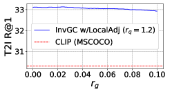
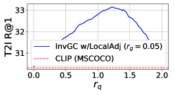
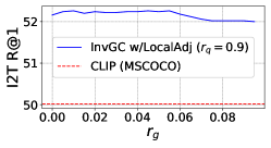
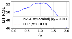
Appendix D Proofs
D.1 Proof of Theorem 1
To prove the theorem, we start with some preliminary definitions. We denote the -dimensional unit sphere as,
and -dimensional ball,
Then, -dimensional ball representing the neighborhood of with radius can be denoted as . We go on to denote spherical caps as
Note that the radius here is not the neighborhood coverage , where they have a relation as by simple triangle calculation. Since the basis of is an dimensional hypersphere of radius and is the key factor we are interested in, we denote the spherical caps using as,
Since the cosine similarity applied is independent of the norm of each point in and , we can assume without loss of generality that all the points in and are on the unit sphere, i.e. . Since query data follows an independent and identical uniform distribution in , therefore it still follows an independent and identical uniform distribution on .
Note that the probability of is correctly retrieved is lower bounded by the probability that the corresponding query point , for must be the nearest neighbor of .
Given uniform distribution, the probability is , where the is the operator for area of hypersurface.
Generally, bounding volume is easier than the surface area, so we have the following Lemma Lemma 3 to help establish the relationship between the two.
Lemma 3.
Therefore, the relationship between the surface area and volumn 555Every time we mention the hypervolume of a sphere where , we actually always refer to that of . We keep using expressions like to prevent possible confusion when dealing with the area and volume at the same time of -dimensional sphere cap is,
| (12) |
Proof.
We have the relationship between the surface area and volume 666When mentioning the hypervolume of a sphere , we actually always refer to that of . of -dimensional unit hypersphere as,
| (13) |
Therefore, the same relationship can be adapted to sphere cap as well. ∎
Theorem 4.
Given -dimensional unit sphere and spherical caps on it, we have,
Proof.
Lower bound: Follow the proof of Lemma 4.1 in Micciancio and Voulgaris (2010). The basis of is an dimensional hypersphere of radius , denoted as . Therefore includes a cone with basis as and height . Then, a cylinder with the same basis but height includes . Note that we have by Taylor expansion. Based on all the facts, we have:
Therefore,
Upper bound: Based on proof of Lower bound, we notice that half of includes , we have
Therefore,
∎
Finally, we finish the proof using Lemma 3.
D.2 Proof of Corollary 2
Proof.
Using the result from Theorem 1, we have the following inequalities for the probability of successful retrieval of and ,
And,
Therefore, we have,
Note that is constant with respect to , so we finish the proof. ∎