Investigation of Numerical Dispersion with Time Step of The FDTD Methods: Avoiding Erroneous Conclusions

Without loss of generality, a homogenous, lossless, isotropic medium and uniform mesh is considered in our study. Therefore, the analytical numerical dispersion of the FDTD(2,2) method [30] can be expressed as

where ${\tilde{k}_{x}}=\tilde{k}\sin\theta\cos\varphi$, $\tilde{k}_{y}=\tilde{k}\sin\theta\sin\varphi$, ${\tilde{k}_{z}}=\tilde{k}\cos\theta$ are numerical wavenumbers in the $x$, $y$ and $z$ direction, respectively, $\theta$ and $\phi$ are the azimuth and zenith angles, $\tilde{k}$ is the numerical wavenumber of electromagnetic waves in the Yee’s grid, $\Delta x$, $\Delta y$ and $\Delta z$ are mesh sizes in the $x$, $y$ and $z$ direction, respectively. $\omega$ denotes the angular frequency and $\Delta t$ is the time step.

To obtain stable numerical solutions for the explicit FDTD (2,2) method, time steps must satisfy the CFL condition [30], expressed as

For convenience in our following derivation, $S_{fdtd(2,2)}$ is defined as

where $\Delta t_{max\_{fdtd(2,2)}}$ is the maximum time step defined by the CFL condition in (3).

The analytical numerical dispersion of the FDTD(2,4) method [30] is written as

Then, the CFL condition for the FDTD(2,4) method [30] is expressed as

We further define $S_{fdtd(2,4)}$ as

where $\Delta t_{max\_{fdtd(2,4)}}$ is the maximum time step constrained by the CFL condition in (6).

Remark 1: $\tilde{k}\geq k$, $\Delta t\in(0,t_{max\_fdtd(2,2)}]$.

Since the explicit expression of $\tilde{k}$ can not be directly obtained from (2), the parameter scanning method [36, 37] is used to study the relationship between $\tilde{k}$ and $k$. We scanned $\theta\in[0,\pi]$, $\phi\in[0,2\pi]$ with other possible parameters in (2). This above statement always holds true. Although it is not mathematically rigorous, it should be enough for practical applications and our analysis. Here, we plot the maximum $\tilde{k}$ with $f=5$ GHz, $\Delta x$ = $\Delta y$ = $\Delta z$ = $6\times{10^{-3}}$ m. Both $\theta\in[0,\pi]$, $\phi\in[0,2\pi]$ are scanned and the maximum $\tilde{k}$ is obtained as shown in Fig. 1. It can be easy to find that when $\Delta t$ satisfies the CFL condition, namely $S\in(0,1]$, $\tilde{k}$ is always larger than $k$.

Lemma 1: For the FDTD(2,2) method,

Proof: Since the explicit expression of $\tilde{k}$ is not available, the implicit differentiation [38] is resorted to investigating the derivative of $\tilde{k}$ with respect to $S$ defined in (4). For convenience of derivations, the following symbols are defined as

and

Therefore, (2) is separated into LHS and RHS two parts. We first consider LHS. By assuming uniform mesh used in the simulations, $\Delta x=\Delta y=\Delta z=\Delta$, and substituting $\omega={{2\pi}}/{{\lambda\sqrt{\varepsilon\mu}}}$ and (4) into LHS, we obtain

where $N$ is the count of sampling cells per wavelength, defined as $N=\lambda/\Delta$. For practical simulations, $N\geq 10$ should be satisfied to obtain acceptable accurate results [30].

With some mathematical manipulations, the derivative of LHS with respect to $S$ is obtained as

where $Q=\left[{\pi S\cos\left({{{\pi S}}/{{\sqrt{3}N}}}\right)-\sqrt{3}N\sin\left({{{\pi S}}/{{\sqrt{3}N}}}\right)}\right]$. Since ${{\pi S}}/({{\sqrt{3}N}})\in(0,{\pi}/{2})$,

Then, let’s check the sign of $Q$ in (12). By taking its derivative, we get

Since $Q$ is a continous function, ${-{\pi^{2}}S\sin\left({\pi S/\sqrt{3}N}\right)/\left({\sqrt{3}N}\right)<0}$, and ${\left.{\left[{\pi\cos\left({{{\pi S}}/{{\sqrt{3}N}}}\right)S-\sqrt{3}N\sin\left({{{\pi S}}/{{\sqrt{3}N}}}\right)}\right]}\right|_{S=0}}=0$, we get

By considering (13), (15) and other variable signs in (12), we can easily get

With a similar manner, the derivative of RHS can be expressed as

where $\tilde{k}=\omega/{\tilde{v}_{p}}$, where $\tilde{v}_{p}$ is the numerical phase velocity in the Yee’s grid, and

with $M={{{\pi a\sin\theta\cos\varphi}}/{N}}$, $T={{{\pi a\cos\theta}}/{N}}$, and $a={c_{0}}/\tilde{v}_{p}$.

To further investigate signs of (18), we divide its domain into several parts based on signs of their function values of each term. Note that the function domain is $\varphi\in[0,2\pi]$ and $\theta\in[0,\pi]$. Therefore, we divide them into several parts to check their signs. The detailed results are summarized in Table I. Table I (a)-(c) correspond to three terms in (18). To better illustrate it, we take term1 in (18) as an example. When $\theta\in\left[{0,\pi/2}\right]$ and $\varphi\in\left[{0,\pi/2}\right]$, it is evidently that $\sin\theta\in\left[{0,1}\right],\cos\varphi\in\left[{0,1}\right]$. Note that $(\pi a/N)\in\left({0,\pi/2}\right)$, then $M\in[{0,\pi/2}]$. Therefore, we have $\sin\left(M\right)\geq 0$ and $\cos\left(M\right)\geq 0$, which implies that term1 is positive when $\theta\in\left[{0,\pi/2}\right]$ and $\varphi\in\left[{0,\pi/2}\right]$. The remaining situations can be obtained with similar manners. To sum them up, we can obtain the following inequality

By considering (16) and (19), we get

Evidently, Lemma 1 is analytically proved and we can further analyze effect of time steps on the NDE of the FDTD(2,2) method.

From Remark 1 and Lemma 1, we can easily find that the numerical wavenumber $\tilde{k}$ monotonically decreases as $S$ in the FDTD(2,2) method increases. When time steps grow larger and are bounded by (3), the numerical phase velocity $\tilde{v}_{p}$ of electromagnetic waves is closer to its physical counterpart $c_{0}$, and then NDE caused by the numerical dispersion would be relatively smaller. Therefore, the NDE reaches its minimum value when $S$ gets its maximum value defined by (3).

With similar procedures, we can investigate effects of time steps upon numerical dispersion for the FDTD(2,4) method.

Remark 2: $\exists t\_\in(0,t_{max\_fdtd(2,4)}]$, we have $\tilde{k}\geq k$, $\Delta t\in(0,t\_],\tilde{k}\leq k$, $\Delta t\in(t\_,t_{max\_fdtd(2,4)}]$.

Lemma 2: For the FDTD(2,4) method,

From Remark 2 and Lemma 2, the NDE $\tilde{k}$ firstly decreases as the $S$ of the FDTD(2,4) method get larger. When $\Delta t\in(t\_,t_{max\_fdtd(2,4)}]$, the NDE becomes larger. Therefore, the NDE reaches its minimum value at $t=t\_$.

To comprehensively investigate the numerical dispersion of the FDTD (2,2) method, the numerical phase velocity $\tilde{v}_{p}$ is calculated from (2). In our numerical studies, the frequency is 5 GHz and $\Delta x$ = $\Delta y$ = $\Delta z$ = $6\times{10^{-3}}$ m, which corresponds to $\lambda/10$. In all other simulations, the same parameters are used, otherwise stated.

As shown in Fig. 2, $\tilde{v}_{p}$ changes periodically over $\varphi$ for a fixed time step $S_{fdtd(2,2)}$ when $\theta=90^{o}$. However, $\tilde{v}_{p}$ increases as $S_{fdtd(2,2)}$ becomes larger with fixed $\phi$ values, which implies that $\tilde{v}_{p}$ approaches $c_{0}$ as time steps grow larger. Therefore, the NDE would become smaller as time steps get larger, which agrees with our analytical analysis in the previous section. Fig. 3 shows $\tilde{v}_{p}$ with respect to $S_{fdtd(2,2)}$ when $\phi=90^{o}$. Similar statements can be also obtained.

Fig. 4 illustrates $\tilde{v}_{p}$ with different $S_{fdtd(2,2)}$ with respect to $\varphi$ and $\theta$. It is easy to find that each $\tilde{v}_{p}$ surface does not intersect each other. Therefore, we can conclude that $\tilde{v}_{p}$ approaches $c_{0}$ as $S_{fdtd(2,2)}$ becomes larger. The numerical dispersion results show that the optimum time step of the FDTD(2,2) method is the largest time step defined by the CFL condition, which also agrees with our theoretical analysis.

$\tilde{v}_{p}/c_{0}$ of the FDTD (2,4) method is also calculated to investigate its numerical dispersion with different $S_{fdtd(2,4)}$. As shown in Fig. 5, $\tilde{v}_{p}/c_{0}$ changes periodically with respect to $\varphi$ when $\theta=90^{\circ}$. $\tilde{v}_{p}$ approaches to $c_{0}$ at the beginning when $S_{fdtd(2,4)}$ becomes large, and then becomes larger than $c_{0}$ as $S_{fdtd(2,4)}$ further increases. Therefore, the NDE of the FDTD (2,4) method firstly decreases and then increases over $S_{fdtd(2,4)}$. The statements obtained in Fig. 6 are similar to those of Fig. 5. They agree with our theoretical analysis.

Here, we provide a numerical method to calculate the optimum time step of the FDTD(2,4) method. The optimum time step is defined as

which can make difference between the numerical wavenumber and its analytical counterpart with $\theta\in[0,\pi]$ and $\varphi\in[0,2\pi]$ minimum.

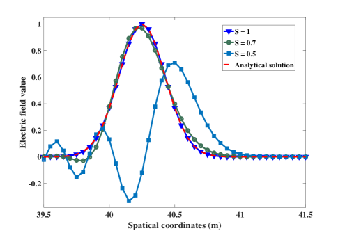
A wave propagation example is used to verify the accuracy of the two FDTD methods with different time steps in one dimensional case. A Gaussian function with the waveform $\phi\left(t\right)={e^{-16{{\left({0.7-ct}\right)}^{2}}}}$ is selected as the excitation, and uniform mesh size $\Delta=5\times{10^{-2}}$ m, and the simulation time is $t=3.6685\times{10^{-8}}$ s. Note that reflected electromagnetic waves do not reach probe in the simulations.

A two dimensional cavity with dimension of $1$ m $\times$ $2$ m and perfectly electric conductor (PEC) boundaries is considered and its resonant frequencies in both transverse magnetic (TM) and transverse electric (TE) modes are calculated through the two FDTD methods. The mesh size is $\Delta=4\times{10^{-2}}$ m.

Case A: a cubic cavity with side length of $1$ m in the three dimensional case is considered. The mesh size is $\Delta=4\times{10^{-2}}$ m. The resonant frequencies are calculated from the two FDTD methods.

Fig. 14 shows the relative error of resonant frequencies obtained from the FDTD(2,2) method. It is similar to one- and two-dimensional cases. Although there are some numerical fluctuations, the relative error becomes smaller for all the three modes as $S_{fdtd(2,2)}$ increases. It agrees well with our investigations.

Fig. 15 shows the resonant frequencies obtained from the FDTD(2,4) method. It is easy to find that relative errors of resonant frequencies show similar behaviors. The relative error gradually decreases and then slightly becomes larger as $S_{fdtd(2,4)}$ become larger. The relative error with small $S_{fdtd(2,4)}$ is larger than that with large $S_{fdtd(2,4)}$. It may account for other numerical errors.

Case B: we use the FDTD(2,2) method to further verify our findings for a practical application in this case. A missile is illustrated by a plane wave and the surface current density is calculated from the FDTD(2,2) method with different time steps. The geometry configurations of the missile in our simulations are shown in Fig. 16(a). It is with dimension of 2.3114$\lambda$$\times$1.4647$\lambda$$\times$0.5334$\lambda$. The plane wave incidents from the $x$-axis with 700 MHz. Fig. 16(b) shows the reference surface current density calculated from the FEKO. Fig. 17(a) and (b) show the surface current density obtained in the FDTD(2,2) method with $S_{fdtd(2,2)}=0.1$ and $1$. It can be found that the surface current distribution obtained from the FDTD(2,2) method agree well with the reference solution. The accuracy of results in our simulations seem unchanged with $S_{fdtd(2,2)}=0.1$ and $1$. There are various factors that can account for those results in this case, like complex geometry, staircase error, possible reflection from the total field/scattered field boundary. It turns out that time steps of the FDTD(2,2) method almost have no significant effects on the accuracy in the practical simulation. Therefore, large time step is preferred in the practical simulations since short simulation time is required and almost the same level of accuracy can also be achieved.

References

- [1] R. J. Luebbers, K. S. Kunz, M. Schneider, and F. Hunsberger, “A finite-difference time-domain near zone to far zone transformation (electromagnetic scattering),” IEEE Trans. Antennas Propag., vol. 39, no. 4, pp. 429-433, 1991.
- [2] M. F. Hadi, M. Piket-May, “A modified FDTD (2,4) scheme for modeling electrically large structures with high-phase accuracy,” IEEE Trans. Antennas Propag., vol. 45, no. 2, pp. 254-264, Feb. 1997.
- [3] A. V. Londersele, D. D. Zutter, and D. V. Ginste, “A new hybrid implicit–explicit FDTD method for local subgridding in multiscale 2-D TE scattering problems,” IEEE Trans. Antennas Propag., vol. 64, no. 8, pp. 3509-3520, Aug. 2016.
- [4] Y. Liu, C. D. Sarris, “Efficient modeling of microwave integrated-circuit geometries via a dynamically adaptive mesh refinement (AMR)-FDTD technique,” IEEE Trans. Microw. Theory Tech., vol. 54, no. 2, pp. 689-703, Feb. 2006.
- [5] C. Kuo, B. Houshmand, “Full-wave analysis of packaged microwave circuits with active and nonlinear devices: an FDTD approach,” IEEE Trans. Microw. Theory Tech., vol. 45, no. 5, pp. 819-826, May 1997.
- [6] F. Xu, K. Wu, and W. Hong, “Domain decomposition FDTD algorithm combined with numerical TL calibration technique and its application in parameter extraction of substrate integrated circuits,” IEEE Trans. Microw. Theory Tech., vol. 54, no. 1, pp. 329-338, Jan. 2006.
- [7] X. Cheng. “Computational Electrodynamics and Simulation in High Speed Circuit Using Finite Difference Time Domain (FDTD) Method,” Ph. D. thesis, ST. Cloud State University, USA, 2018.
- [8] J. Mix, G. Haussmann, M. Piket-May and K. Thomas, “EMC/EMI design and analysis using FDTD,” in Proc. IEEE Intl. Symposium on EMC, vol. 1, pp. 177-181, Aug. 1998.
- [9] J. Chen, J. Wang, “A three-dimensional semi-implicit FDTD scheme for calculation of shielding effectiveness of enclosure with thin slots,” IEEE Trans. Electromagn. Compat., vol. 49, no. 2, pp. 354-360, 2007.
- [10] R. Matsubara, K. Inokuchi, “Development of EMC analysis technology using large-scale electromagnetic field analysis,” in 2019 41st IEEE Annual EOS/ESD Symposium (EOS/ESD), pp.1-6, Sep. 2019.
- [11] D. M. Hockanson, X. Ye, J. L. Drewniak, T. H. Hubing, T. P. VanDoren and R. F. DuBoff, “FDTD and experimental investigation of EMI from stacked-card PCB configurations,” IEEE Trans. Electromagn. Compat., vol. 43, pp. 1-10, Feb. 2001.
- [12] A. Yash, R. Chandel, “Crosstalk analysis of current-mode signalling-coupled RLC interconnects using FDTD technique,” IETE Technical Review, vol. 33, no. 2, pp.148-159, 2016.
- [13] B. R. Archambeault, O. R. Ramahi, C. Brench, EMI/EMC computational modeling handbook (Vol. 630) . Springer Science Business Media, 2012.
- [14] W. Yu, R. Mittra, T. Su, Y. Liu, and X. Yang, Parallel finite-difference time-domain method. Artech House, 2006
- [15] W. Yu, X. Yang, Y. Liu, R. Mittra, D. -C. Chang, C. -H. Liao, A. Muto, W.Li, and L. Zhao, “New development of parallel conformal FDTD method in computational electromagnetic engineering,” IEEE Antennas Propag. Mag., vol. 53, no. 3, pp. 15-41, Sep. 2011.
- [16] K. Lan, Y.W. Liu, and W. G. Lin, “A higher order (2,4) scheme for reducing dispersion in FDTD algorithm,” IEEE Trans. Electromagn. Compat., vol. 41, no. 2, pp. 160-165, May 1999.
- [17] W. Fu, E. L. Tan, “Development of split-step FDTD method with higher-order spatial accuracy,” Electron. Lett., vol. 40, no. 20, pp. 1252-1254, Sep. 2004.
- [18] Q. F. Liu, Z. Chen, and W. Y. Yin, “An arbitrary order LOD-FDTD method and its stability and numerical dispersion,” IEEE Trans. Antennas Propag., vol. 57, no. 8, pp. 2409-2417, Aug. 2009.
- [19] T. Namiki, “A new FDTD algorithm based on alternating-direction implicit method,” IEEE Trans. Microw. Theory Tech., vol. 47, no. 10, pp. 2003-2007, Oct. 1999.
- [20] F. Zheng, Z. Chen, and J. Zhang, “Toward the development of a three-dimensional unconditionally stable finite-difference time-domain method,” IEEE Trans. Microw. Theory Tech., vol. 48, no. 9, pp. 1550-1558, Sep. 2000.
- [21] J. Shibayama, M. Muraki, J. Yamauchi, and H. Nakano, “Efficient implicit FDTD algorithm based on locally one-dimensional scheme,” Electron. Lett., vol. 41, no. 19, pp. 1046-1047, Sep. 2005.
- [22] F. Zheng, Z. Chen, “Numerical dispersion analysis of the unconditionally stable 3-D ADI-FDTD method,” IEEE Trans. Microw. Theory Tech., vol. 49, no. 5, pp. 1006-1009, May 2001.
- [23] I. Ahmed, E. K. Chun, and E. P. Li, “Numerical dispersion analysis of the unconditionally stable three-dimensional LOD-FDTD method,” IEEE Trans. Antennas Propag., vol. 58, no. 12, pp. 3983-3989, Dec. 2010.
- [24] E. Li, I. Ahmed, and R. Vahldieck, “Numerical dispersion analysis with an improved LOD-FDTD method,” IEEE Microw. Wireless Compon. Lett., vol. 17, no. 5, pp. 319-321, Apr. 2007.
- [25] J. Pereda, O. Garcia, A. Vegas, and A. Prieto, “Numerical dispersion and stability analysis of the FDTD technique in lossy dielectrics,” IEEE Microwave Guided Wave Lett., vol. 8, no. 7, pp. 245–247, Jul. 1998.
- [26] J. B. Schneider, C. L. Wagner, “FDTD dispersion revisited: Faster-than-light propagation,” IEEE Microwave Guided Wave Lett., vol. 9, no. 2, pp. 54-56, 1999.
- [27] Z. T. Theodoros , T. D. Tsiboukis, “Low-dispersion algorithms based on the higher order (2, 4) FDTD method,” IEEE Trans. Microw. Theory Tech., vol. 52, no. 4, pp.1321-1327, 2004.
- [28] S. C. Yang, Z. Chen, Y. Yu, and W. Y. Yin “An unconditionally stable one-step arbitrary-order leapfrog ADI-FDTD method and its numerical properties,” IEEE Trans. Antennas Propag., vol. 60, no. 4, pp. 1995-2003, Apr. 2012.
- [29] S. J. Cooke, M. Botton, T. M. Antonsen, and B. Levush, “A leapfrog formulation of the 3D ADI-FDTD algorithm,” Intl. Workshop on Computational Electromagnetics in Time-Domain, pp. 1-4, Oct. 15-17, 2007.
- [30] A. Taflove, S. C. Hagness. Computational Electrodynamics: The Finite-Difference Time-Domain Method. Norwood, MA: Artech House, 2005
- [31] S. J. Jaakko, T. D. Tsiboukis, “Reduction of numerical dispersion in FDTD method through artificial anisotropy,” IEEE Trans. Microwave Theory Tech., vol. 48, no. 4, pp. 582-588, Apr. 2000.
- [32] I. Ahmed, Z. Chen, “Dispersion-error optimized ADI FDTD,” Proc. IEEE MTT-S Int. Microw. Symp. Dig., vol. 2006, pp. 173–176, Jun. 2006.
- [33] Q. F. Liu, W. Y. Yin, Z. Chen, and P. G. Liu, “An efficient method to reduce the numerical dispersion in the LODFDTD method based on the (2, 4) stencil,” IEEE Trans. Antennas Propag., vol. 58, no. 7, pp. 2384-2393, Jul. 2010.
- [34] G. Chen, S. Yang, Q. Ren, S. Cui, and D. Su, “Numerical dispersion reduction approach for finite-difference methods,” Electron. Lett., vol. 55, no. 10, pp. 591-593, 2019.
- [35] T. T. Zygiridis, “Optimum time-step size for 2D (2, 4) FDTD method,” Electron. Lett., vol. 47, no. 5, pp. 317–319, Mar. 2011.
- [36] X. H. Wang, J. Y. Gao, Z. Z. Chen, and F. L. Teixeira. “Unconditionally stable one-step leapfrog ADI-FDTD for dispersive media,” IEEE Trans. Antennas Propag., vol. 67, no. 4, pp. 2829-2834, Apr. 2019.
- [37] G. Z. Chen, S. C. Yang, and D. L. Su. “An accurate three-dimensional FDTD (2, 4) method on face-centered cubic grids with low numerical dispersion,” IEEE Antennas Wireless Propa. Lett. vol. 18, no. 9, pp. 1711-1715, Sept. 2019.
- [38] G. Strang. Calculus. MA: Wellesley College, 1991.