Investigation of neutron imaging applications using fine-grained nuclear emulsion
Abstract
Neutron imaging is a non-destructive inspection technique with a wide range of applications. One of the important aspects concerning neutron imaging is achieving micrometer-scale spatial resolution. Developing a neutron detector with a high resolution is a challenging task. Neutron detectors, based on fine-grained nuclear emulsion, may be suitable for high resolution neutron imaging applications. High track density is a necessary requirement to improve the quality of neutron imaging. However, the available track analysis methods are difficult to apply under high track density conditions. Simulated images were used to determine the required track density for neutron imaging. It was concluded that a track density of the order of tracks per 100 100 m2 is sufficient to utilize neutron detectors for imaging applications. The contrast resolution was also investigated for the image data sets with various track densities and neutron transmission rates. Moreover, experiments were performed for neutron imaging of the gadolinium-based gratings with known geometries. The structure of gratings was successfully resolved. The calculated 1 10-90 % edge response, using the gray scale optical images of the grating slit with a periodic structure of 9 m, was 0.945 0.004 m.
I Introduction
Neutron imaging (NI) is a non-destructive technique for visualizing and analysing the inner structure of material objects. It has a wide range of applications Strobl and et al. (2009); Hussey and Jacobson (2015); Lehmann and et al. (2015); Kardjilov and et al. (2018); Tengattini et al. (2021); Song and et al. (2019); Lv and et al. (2018). The basic principle for NI is similar to that of X-ray imaging. Neutrons are neutral particles and can interact directly with atomic nuclei. The absorption and scattering cross-sections of neutrons depend on the nuclides. The dependence of attenuation coefficients of neutrons is different from that of X-rays which is correlated to the atomic number Banhart (2008). Contrary to X-rays, neutrons exhibit high attenuation for light (e.g. hydrogen, carbon, boron and lithium) and heavy (e.g. cadmium and gadolinium) nuclei. Lower attenuation is observed for heavy nuclei including aluminum, silicon, titanium and lead. These characteristics give neutron imaging an advantage over X-ray imaging. Neutron imaging may be employed as an effective method to visualize distributions for a wide range of elements using the difference in their neutron attenuation coefficients Strobl and et al. (2009).
The major challenges in developing NI techniques include improvements in spatial resolution Tremsin and et al. (2011); Hussey and et al. (2015); Trtik and et al. (2015); Trtik and Lehmann (2016); Bingham and et al. (2015); Morgano and et al. (2018); Trtik and et al. (2020), detection efficiency, Tremsin and et al. (2011) and time resolution Kardjilov and et al. (2018); Woracek and et al. (2019) of neutron detectors. Recent developments have improved the spatial resolution of NI to a few micrometers. One of the common approaches in NI is to convert the shading field of the neutron beam into an image of visible light using scintillators containing converters such as 6Li or 157Gd Trtik and et al. (2020); Lehmann and et al. (2011); Hussey et al. (2017); Jiang and et al. (2021). The luminescence of a neutron capture event was observed by a charge–coupled device (CCD) or a complementary metal-oxide-semiconductor (CMOS) image sensor via an optical system. Using a technique based on this approach, the best resolution resolution currently reported is 2 m Hussey et al. (2017). This spatial resolution was achieved using a thin gadolinium oxysulfide scintillator, magnifying optics, a CMOS image sensor, and an event positioning method by detecting the center of the luminescence for each event. Isegawa et al.Isegawa and et al. (2021) used a Gd3Al2Ga3O12:Ce single-crystal scintillator for the neutron radiography and achieved a spatial resolution of 10.5 m.
For micrometer-scale spatial resolution or even better, nuclear emulsion is one of the potential candidates for NI device. Nuclear emulsion is a photographic film that can record the three-dimensional trajectories of charged particles with submicrometer-scale spatial resolution. It is composed of silver halide (AgBr) crystals dispersed in gelatin. Nuclear emulsions were initially developed for particle and nuclear physics experiments to observe the tracks of charged particles. They were used to observe pions Lattes, Occhialinidr, and Powelldr (1947), hypernuclei Danysz and Pniewski (1953); Davis (2005), charm particles Niu, Mikumo, and Maeda (1971) and double strangeness hypernuclei Danysz and et al. (1963). The analysis speed of nuclear emulsions has increased remarkably with improvements in image processing techniques Yoshimoto et al. (2017); Saito and et al. (2017). These improvements enable the use of nuclear emulsion in modern experiments, and led to the first direct detection of tau-neutrinos Kodama and et al. (2001), discovery of oscillations in appearance mode Agafonova and et al. (2015), hypernuclei Saito and et al. (2017); Hiyama and Nakazawa (2018); Ekawa and et al. (2019); Hayakawa and et al. (2008); Yoshimoto and et al. (2021) and for several other applications including muon radiography Tanaka and et al. (2007); Morishima and et al. (2017).
Since the last decade, it has become possible to produce dedicated nuclear emulsions for specific purposes. Controlling the size of the AgBr crystals and chemical components contributed in achieving optimal spatial resolution and sensitivity. Fine-grained nuclear emulsions (FGNEs) with AgBr crystals, having a diameter of less than 50 nm, was developed Naka and et al. (2013); Asada et al. (2017) to detect the tracks of the nuclei recoiled by the so-called weakly interacting massive particles. The sensitivity of the nuclear emulsion was optimised to track the nuclei but was maintained sufficiently low for electrons and -rays Shiraishi and et al. (2021).
The FGNE with crystal diameter of 40 nm was employed for cold/ultracold neutron detection by combining it with a neutron converter layer formed by 10B4C. This layer absorbs neutrons and emits two charged particles heading in the opposite direction via the following process: 10B + n 7Li + 4He. When one of the emitted ions passes isotropically through an emulsion layer, latent image specks are created in some AgBrI crystals along its trajectory. After the chemical development, each crystal that contains latent image specks changes to an enlarged silver grain. A series of these grains is recognized as a track of the charged particle. Naganawa et al.Naganawa and et al. (2018) reported the development of a cold/ultracold neutron detector using FGNE and that the spatial resolution of neutron absorption points was estimated as less than 0.1 m from linear fitting of tracks. The track lengths of 7Li and 4He recorded in the emulsion layer were 2.6 0.4 and 5.1 0.4 m, respectively. This development was initiated for fundamental physics experiments to investigate quantized states under the influence of the earth’s gravitational field and to search unknown interactions attracting neutrons Nesvizhevsky and et al. (2002); Abele et al. (2009); Ichikawa and et al. (2014); Muto and et al. (2022).
The FGNEs combined with a boron-based neutron converter can be applied for NI applications. For the purpose of NI, the accumulated track density must be several orders of magnitude higher than that used in ref. Naganawa and et al. (2018). Hirota et al. Hirota and et al. (2021) demonstrated NI of a crystal oscillator chip using FGNE under the accumulated track density of tracks per 100 100 m2. They used a similar NI detector as in ref. Naganawa and et al. (2018), but the thickness of 10B4C layer was 2 m to increase neutron conversion efficiency. The thickness of 10B4C layer used for neutron detection in ref. Naganawa and et al. (2018) was 50 nm. Gold wires with a diameter of approximately 30 m in the crystal oscillator chip were successfully visualized. Furthermore, they attempted NI of a gadolinium-based grating with a periodic structure of 9 m under the accumulated track density of tracks per 100 100 m2. They confirmed the grating spacing of 9 m pitch using Rayleigh test with a standard deviation of 1.3 m. They concluded that the achievable resolution for the NI using the FGNE was better than 3 m. The challenges presented in ref. Hirota and et al. (2021) were to develop a method of image analysis and spatial resolution under a condition of tracks per 100 100 m2. With such a high track density, the conventional track-by-track analysis becomes difficult because of the overlap of the tracks.
For NI, the neutron detector based on the FGNE combined with neutron converter has several merits. It can detect neutron capture events with submicrometer-scale spatial resolution. The detector is lightweight, thin, small ( adjustable to sample objects with an area of approximately 100 cm2), and does not require any electric supply or drive in electronics. Furthermore, this detector can be integrated into devices or sample environment apparatus to shorten the distance with the investigated object. It can be added to existing imaging systems without any major modification and may be used as a complementary imaging device. Along with these merits, there are several limitations as well. A longer beam exposure time is required for a thinner 10B4C layer in order to achieve higher spatial resolution. An additional process of chemical development is required after exposure. Furthermore, this detector is unsuitable for real-time measurements and applications where neutron energy measurement is required.
For NI applications using the FGNE, a high density accumulated tracks is a basic requirement. We describe our detector in section II. The estimation of track density and diffuseness as a metric to evaluate the imaging resolution is discussed in section III.1. The procedure employed to investigate the contrast resolution is discussed in section III.2. The details of the experiments are discussed in section IV. The results for NI of gadolinium-based gratings are discussed in section V. The NI application of the FGNE is discussed in the section VI. We finally conclude our findings and discuss future prospects in section VII.
II Neutron detector
The neutron detector developed for this work, shown in Figure 1a, has a layered structure. The base of the detector is a 0.4 mm thick silicon substrate. On this substrate, 10B4C, NiC and C layers of thicknesses 230 nm, 46 nm and 14 nm, respectively, were formed by ion beam sputtering technique Hino and et al. (2015). The thickness of the 10B4C layer was determined by taking into account neutron detection efficiency, the physical stability, and the spatial resolution for the imaging. The 10B4C layer converts an incident neutron into 4He and 7Li. The NiC layer was used to physically stabilise the 10B4C layer. The C layer was used for chemical protection from the NiC layer and for providing a strong adhesion to the emulsion. An emulsion layer of thickness 10 m was formed on the sputtered layers in a dark room by pouring and drying the FGNE. It was composed of AgBrI crystals of approximately 40 nm diameter uniformly dispersed in medium including gelatin and polyvinyl alcohol. The neutron detector was packed with a light- and air-tight laminated bag, composed of nylon, polyethylene, aluminum, polyethylene and black polyethylene layers having thicknesses of 15 m, 13 m, 7 m, 13 m and 35 m, respectively. During the beam exposure, the detector and the gadolinium-based grating were placed close together to minimise the blurring effects induced by the spreading of transmitted neutron beam, as shown in Figure 1a. Some incident neutrons were absorbed in the grating, and remaining neutrons were absorbed in the 10B4C layer. When a 10B nucleus absorbs a neutron, the reaction products, 4He and 7Li, are emitted head off in opposite directions. When one of them passes through the emulsion layer, latent image specks are created in AgBrI crystals along its trajectory. After chemical development, crystals containing latent image specks transform to silver grains. Figure 1b shows a photograph of the detector after the chemical development. After chemical development, the thickness of the emulsion layer shrinks by a factor of 0.55 0.1. A set of gray scale images were obtained with submicrometer precision using an epi-illumination optical microscope. The series of silver grains in these images is recognized as the induced tracks of the charged particles.

III Simulations for imaging applications
Tracks of 4He and 7Li have certain length as they travel through the nuclear emulsion. If the track density is high ( tracks per 100 100 m2), they blot out the edge of the object in the obtained images. On the other hand, if the track density is low ( tracks per 100 100 m2), the outline of the object will not be visible. Therefore, it was important to estimate the required track density for NI, and diffuseness as a function of track density for the current NI system. The track density required for NI, and diffuseness was estimated using simulated images which we present below.


III.1 Estimation of track density
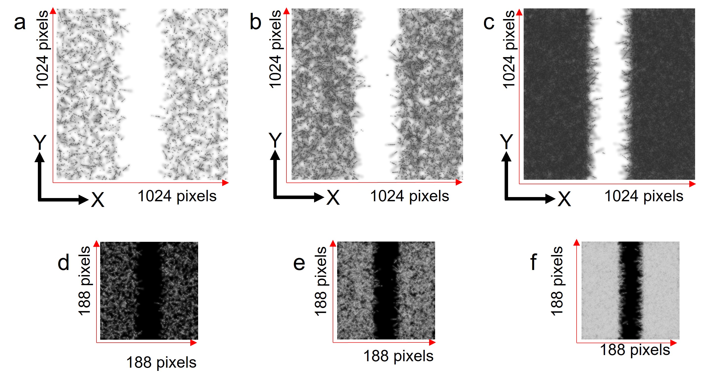
Data sets of simulated images were generated under several track density conditions ranging from to tracks per 100 100 m2. Each data set contained 165 images. The images are shown in Figures 2a, 2b and 2c for track densities of , and tracks per 100 100 m2, respectively. Each simulated image had a single bar pattern with a width of 15 m where the incidents neutrons are absorbed. Since the track length of 4He recorded in the emulsion layer was 5.1 0.4 m Naganawa and et al. (2018), the width of single bar pattern was taken as 15 m. As shown in the Figure 2c, decrease in the width of the bar pattern is visible which is due to finite length of the tracks with an increase in the track density. The simulated images were scaled down to 188 pixels 188 pixels using the nearest neighbor method Rukundo and Cao (2012) where size of one pixel is equivalent to 0.3 m (typical diameter of a silver grain). Figures 2d, 2e and 2f show resized and inverted images of Figures 2a, 2b and 2c, respectively. The trapezoid fitting for the projection of brightness sum of the corresponding resized and inverted images is shown in Figures 3a, 3b and 3c, respectively. The width of single bar pattern was defined as the distance between the midpoints of the slopes of the trapezoid fitting curve. The edge response defined as L(10-90%) was deduced as the distance between 10 % and 90 % of the knife edges of the trapezoid fitting curve as shown in Figure 4.
The length of the statistical error bar of each data point is shown in Figures 3a, 3b and 3c. The errors were estimated using the following procedure. Data sets of simulated images were created under several track density conditions ranging from 1 track per 100 100 m2 to tracks per 100 100 m2. Simulated images under track density of and tracks per 100 100 m2 are shown in Figures 5a and 5b, respectively. These simulated images were scaled down to 188 pixels 188 pixels as discussed above. The mean and standard deviation values (shown in Figures 6a and 6b) were calculated from the brightness sum distribution of the resized images (shown in Figures 5a and 5b). Figure 7a shows the deduced standard deviation values as function of corresponding brightness values, while the blue curve shows the polynomial fitting. The deduced standard deviation values were employed as the length of error bar for the corresponding brightness values (shown in Figures 3a, 3b and 3c). Figure 7b shows the brightness sum values as a function of track densities. The brightness sum was almost saturated in a high track density region around tracks per 100 100 m2.


The resolved width and L(10-90%) edge response (displayed in Figure 4) were used to evaluate the diffuseness as a function of track density as shown in Figures 8a and 8b, respectively. The length of error bar for each data point in these figures was estimated as standard deviation of corresponding brightness values. As the track density increases, the resolved width of the grating decreases due to finite length of the tracks in the FGNE. As shown in Figure 8a, a track density of tracks per 100 100 m2 is sufficient for imaging applications using the current FGNE based NI system (also discussed in section II). The L(10-90%) edge response (shown in Figure 8b) is relatively constant, and diffuseness of 3.33 0.27 m can be achieved under the accumulated track density of tracks per 100 100 m2 for NI using the FGNE.


III.2 Contrast resolution
It is equally important to investigate the contrast resolution for the imaging applications using the FGNE. To investigate the contrast resolution, image data sets with track densities , , , , and per 100 100 m2 were generated with neutron transmission rates of 70 %, 75 %, 80 %, 85 %, 90 %, 95 %, 96 %, 97 %, 98 % and a data set with 100 % transmission. Figures 9a, 9b and 9c show the simulated images under the accumulated track density of , and per 100 100 m2, respectively, for the neutron transmission rate of 95 %. The average brightness values in area ranging from 20, 21, …. , up to 213 m2, under the given neutron transmission, were compared with the corresponding average brightness values with the neutron transmission of 100 %. Figures 10 show the comparison of the average brightness values for the combination of 100 % vs. 96 % neutron transmission rate under the accumulated track density of per (100 m)2. The area capable of separation at least per m2 was 2048 m2. The results of the contrast resolution for the combination of 100 % vs. various neutron transmission rates under the accumulated track densities are summarized in Table 1. Corresponding figures for the contrast resolution of each image data set, at the given neutron transmission rates and track densities, are shown in Appendix A.
The simulation result for the image data sets with neutron transmission rate of 96 % under the accumulated track density of tracks per 100 100 m2 is shown in Table 1 and Figure 10. The simulation-based results can be compared with the results of NI of the gold wires in a crystal oscillator chip using the FGNE Hirota and et al. (2021). Hirota et al. visualized the gold wires with a diameter of 30 m and length 1 mm under the accumulated track density of tracks per 100 100 m2 and neutron absorption rate of 3.84 %. For neutron transmission rate of 96 %, the area which can be resolved is 2048 m2 as shown in Table 1 and Figure 10 and it is concluded that an object with an area much smaller than gold wire with a diameter of 30 m and length 1 mm may be resolved using the FGNE.
| Trans. | 3 | ||||||
|---|---|---|---|---|---|---|---|
| 100 % vs. | 70 % | 1024 | 256 | 64 | 16 | 2 | 1 |
| 75 % | 1024 | 256 | 64 | 64 | 8 | 1 | |
| 80 % | 2048 | 256 | 256 | 64 | 8 | 4 | |
| 85 % | 4096 | 1024 | 256 | 64 | 16 | 8 | |
| 90 % | 8192 | 4096 | 512 | 512 | 64 | 32 | |
| 95 % | 8192 | 4096 | 2048 | 512 | 128 | ||
| 96 % | 8192 | 2048 | 512 | 128 | |||
| 97 % | 4096 | 1024 | 256 | ||||
| 98 % | 8192 | 2048 | 512 |
IV Experiments
For the neutron irradiation, we used the low-divergence beam branch Mishima and et al. (2009) of BL05 in the Materials and Life Science Experimental Facility (MLF) at the Japan Proton Accelerator Research Complex (J-PARC) Nakajima and et al. (2017). This is one of the most suitable beam branches in the MLF for this experiment because it provides a reasonably intense neutron beam owing to a coupled neutron moderator.
For NI of the gadolinium-based grating slit, the aperture of the slit was 44 mm and 6 mm for the horizontal and vertical directions, respectively. The beam divergence in the horizontal and vertical directions was set to 0.3 mrad and 10 mrad, respectively. It is to be noted that the beam divergence parallel to the grating does not affect the blurring of the image. The neutron flux was n/cm2/s, and the neutron irradiation time was 2.8 h to accumulate approximately tracks per (100 m)2. The distance between the gadolinium-based grating and the 10B4C layer was 1.5 mm. The detector and the grating were fixed by metal clips and mounted on a holder for optical elements on an optical table.
On the other hand for imaging applications using the FGNE, NI of the Siemens star test pattern was also performed. The aperture of the slit on the 12 m position was set to 4 mm and 6 mm for the horizontal and vertical directions, respectively, to avoid blurring due to vertical divergence. The corresponding horizontal and vertical divergences of the beam were 0.3 mrad and 1.0 mrad, respectively. The typical beam power and the neutron flux during the experiment were 0.7 MW and n/cm2/s, respectively. The irradiation time was 9 h to accumulate tracks per (100 m)2. The distance between the gadolinium layer of the Siemens star and the 10B4C layer in the detector was 1.1 mm. The NI experiments for the grating slit and the Siemens star test patter were carried out under a stable environmental temperature of 23.9 0.1 ∘C.
IV.1 Scanning the emulsion in the neutron detector
A dedicated optical microscope with an epi-illumination system was used to scan the emulsion layer on a non-transparent silicon substrate. The light source of this system was a 1 W LED with a wavelength of 455 nm. The objective lens was an oil-immersion type with a magnification of 100x with a numerical aperture (NA) of 1.45 (Nikon Plan Apo). The depth of field was derived as / NA 0.43 m. The focusing unit of this microscope system was controlled by a stepping motor. The microscope system acquired a set of sequential images along the optical axis with a pitch of 0.3 m from the upper to the lower boundary of the emulsion layer with enough margin. The typical number of images to be taken at a certain place was 63. To scan the specified volume of the emulsion layer in three dimensions, the system shifted the field of view in the horizontal direction at a 50 m pitch by the two other stepping motors and repeated the image acquisition. These images were acquired as 8-bit gray scale images with a CMOS image sensor with 2048 pixels 2048 pixels (SENTECH CMB401PCL) at speeds of up to 160 frames per second. The length of one side of the field of view was approximately 112 m. Accordingly, a single-pixel corresponded to 0.055 m. Optical aberration in the periphery of the field of view reduces the quality of the image. We, therefore, used the central region of the acquired gray scale image (i.e., 1024 pixels 1024 pixels).
V Results
V.1 Gadolinium grating
The grating slit with a periodic structure of 9 m was used for the NI using the FGNE, which was made for a Talbot–Lau interferometer for neutron phase imaging Seki and et al. (2017). Figure 11a shows the image of the gadolinium-based grating slit. It was formed on a 525 m-thick silicon substrate and mounted at the centre of a 525 m-thick five-inch silicon wafer. Figure 11b is a scanning electron microscopy (SEM) image of a similar grating slit. A periodic structure of 9 m (111 line pairs per mm) was formed on the silicon substrate. Figure 11c is the SEM image of the cross-section of a gadolinium tooth of same type, while Figure 11d shows a schematic view of the gadolinium teeth. Gadolinium teeth with a width of approximately 5 m and empty spaces of 4 m were formed periodically. The shape of gadolinium tooth was not a perfect rectangular structure mainly because of the production process Samoto, Takano, and Momose (2019a, b). Such grating can provide an inclusive assessment of the diffuseness including the effects of the resolution of the detector and imperfect shape of the gadolinium teeth. Each tooth was formed by depositing gadolinium from an oblique angle onto the ridge-like structures formed on the silicon substrate Seki and et al. (2017). The direction of the irradiated neutron beam was from left to right. A portion of the incident neutron beam was absorbed by the gadolinium, while the remaining beam passed through the empty spaces. Figure 11e shows a micrograph of tracks recorded in the emulsion layer. The dimensions and number of pixels of this image are 56 m 56 m and 1024 pixels 1024 pixels, respectively. The periodic structure of gadolinium grating with 9 m was clearly resolved and is visible.

V.2 Image processing
The acquired gray scale optical images of the grating slit were further processed. The raw data obtained by the optical microscope were a set of 63 sequential images with 2048 pixels 2048 pixels for each field of view. These optical images contained shades of dust on the image sensor and non-uniformity of the brightness due to optical conditions. In order to extract shades of dust, the average brightness for each pixel in the 63 sequential images was calculated. To remove shades of dust and non-uniformity of the brightness, the pixel brightness value of each optical image was divided by the calculated average brightness value of the corresponding pixel. This image processing was applied to the image data sets for 165 field of views. The images at the depth of the boundary between the sputtered carbon layer and the emulsion layer were selected for further analysis. The inner portion of 1024 pixels 1024 pixels was cropped in these images.
V.3 10-90 % edge response evaluation
The L(10-90%) edge response (shown previously in Figure 4) of the grating slit with a periodic structure of 9 m was evaluated using the simulated and optical images. The image processing, as explained in the previous subsection, was employed to the optical images. Figures (12a and 14a) show the simulated and optical images of the grating slit, respectively. Figures (12b and 14b) show the inverted image of Figures (12a and 14a, respectively). The inverted images were scaled down to 188 pixels 188 pixels as discussed in the subsection III.1 and displayed in Figures (12c and 14c, respectively). Using these resized images, the brightness sum in the direction parallel to the grating (Y-direction) were calculated at specified X-value with a range of bin sizes. The green lines in Figures (13a and 15a) show the defined boundary positions of the peaks and valleys of each edge section in the simulated and real images, respectively. The data points between the two consecutive peaks were extracted and trapezoid fitting was employed in the subsequent analyses to calculate the L(10-90%) edge response for evaluation of the diffuseness. For example, five edges were extracted from each image shown in Figures (13a and 15a). Figures (13b and 15b) show the trapezoid fitting for the extracted data points. The red dotted lines in these figures show the fitting curves. The length of each error bar (shown in Figures 13b and 15b) was estimated in a way similar to that explained in subsection III.1. Figures (16a and 16b) show the distributions of the reduced of the fitting for the simulated and optical images, respectively. Figures (17a and 17b) show the distribution of L(10-90%) edge diffuseness for the simulated and optical images, respectively. The 1 of L(10-90%) edge diffuseness was calculated for the inclusive assessment of the resolution. The red dotted lines in these images show the Gaussian fitting curve. The deduced values of the diffuseness distributions for simulated and optical images were 2.21 0.01 and 2.42 0.01 m, respectively. The L(10-90%) edge response in 1 for the simulated and optical images were 0.863 0.004 m and 0.945 0.004 m, respectively. The resolution of 0.945 0.004 m is an inclusive assessment that includes the effects of the resolution of the detector and the shape of the gadolinium tooth. Therefore this deduced resolution is the upper limit of the actual resolution, and might be better than the deduced resolution. Submicrometer spatial resolution maybe achieved using a fine-grained nuclear emulsion for neutron imaging because the deduced resolution is less than 1 m.
As mentioned in subsection II, the emulsion layer shrunk by a factor of 0.55 0.1 after chemical development. With a shrinkage factor of 0.55, the deduced value of the diffuseness distribution for simulated images was 2.21 0.01. In order to calculate the systematic error induced due to the shrinkage of the emulsion layer, additional simulated image data sets, with a shrinkage factor of 0.4 and 0.6, were generated. The deduced value of the diffuseness distribution was .
The grating slit in the simulated images had a perfect rectangular structure. A fair agreement was observed between the diffuseness values of the simulated and optical images. As discussed in subsection V.1, the grating slit did not posses a perfect rectangular structure. The slight difference in the diffuseness values could be attributed to the imperfectness in the shape of the grating slit. The calculated diffuseness was in fair agreement for the simulated and optical images. Consequently the achievable diffuseness under the accumulated track density of tracks per 100 100 m2 can be 3.33 0.27 m for NI of a simple bar like structure using the FGNE.


VI Demonstration of imaging application using FGNE
As discussed in the section IV, NI of the Siemens star test pattern was performed for the demonstration one of the applications of the proposed NI system. Figure 18a shows a photograph of the Siemens star test pattern used in our experiments. This pattern was designed by a group in the Paul Scherrer Institute (PSI), Villigen, Switzerland. A prototype of the test pattern is described in Ref. Grünzweig and et al. (2007). The pattern consisted of 128 spokes in a circular area of 20 mm diameter and was made of a thin layer ( 5 m) of gadolinium on a quartz wafer of thickness 0.7 mm. The space between the spokes became narrower towards the center of the circle. The innermost spoke had a period of 10 m, which corresponds to 100 line pairs per millimeter. Figure 18b shows an optical image of the Siemens star test pattern using optical microscope with a trans-illumination system with a magnification of 20x, and a numerical aperture (NA) of 0.35.
The spatial resolution of an imaging device is assessed by the fine resolution of the intervals of the inner spokes. Figure 18b shows a photograph of the developed detector irradiated with the neutron beam through the pattern. The pattern transferred on the emulsion layer is visible to the naked eye even before being observed under an optical microscope. The dark regions correspond to the sites where silver grains were developed by the emitted 4He or 7Li during the neutron absorption events. Other regions correspond to sites where the neutrons were absorbed by gadolinium on the pattern. The neutron absorption events in the 10B4C layer were suppressed. Figure 18c shows an image of the nuclear emulsion, which recorded the thinnest spokes near the center of the pattern. As shown in Figure 18b, the grating is not very well fabricated therefore the diffuseness for the edges of the grating was not evaluated quantitatively. One can note that the innermost spokes are clearly resolved as shown in Figure 18d. Our NI results shows the ability of the FGNE to resolve the micrometer-scale structures with micrometer-scale resolution or even better.

VII Summary and outlook
In this work, we presented the simulated results of neutron imaging using the fine-grained nuclear emulsion. It was concluded that a track density of tracks per 100 100 m2 was required for neutron imaging applications. The contrast resolution was investigated for various track densities under varying conditions of neutron transmission rates. Our results estimated a contrast resolution and area capable of separation 1 per (m2) under various accumulated track densities per (100 m)2 and varying neutron transmission rates for the current neutron imaging system.
The neutron imaging of gadolinium-based gratings with known geometries, such as a Siemens star test pattern and a grating slit with a periodic structure of 9 m, were further reported in this work. These micrometer structured gratings were imaged and resolved successfully. The evaluated diffuseness for the edges of the grating slit under high accumulated track density conditions, for simulated and optical images, were 0.863 0.004 m and 0.945 0.004 m, respectively. The difference in the diffuseness values may be attributed to the shape of the gadolinium teeth. It is reminded that the grating slit is not a perfect rectangular structure because of the production process, as described in Ref. Samoto, Takano, and Momose (2019a, b). The diffuseness values for simulated and optical images were in fair agreement and it may be concluded that the achievable resolution under the accumulated track density of tracks per 100 100 m2 is 0.945 0.004 m. The obtained resolution for the optical images is an inclusive assessment that includes the effects of the resolution of the detector and the shape of the gadolinium tooth. It is concluded that the actual resolution may be better than the deduced resolution, and neutron imaging with submicrometer spatial resolution can be performed using the neutron detection system based on the fine-grained nuclear emulsion. In future, we plan to perform experiments for the exclusive assessment of simpler structure and evaluate the spatial resolution of the proposed neutron imaging system including neutron imaging of material objects.
Acknowledgements.
The neutron experiment at the Materials and Life Science Experimental Facility of the J-PARC was performed under user programs (Proposal No. 2020B0223). The preliminary experiment on the detector was performed at the Research Reactor Institute, Kyoto University (Experiment No. R2138). J. Y. was supported by JSPS KAKENHI Grant Number JP18H05403 (Grant-in-Aid for Scientific Research on Innovative Areas 6005). The authors thank Takenao Shinohara of J-PARC and Yoshichika Seki of Tohoku University for lending the Siemens star test pattern and the grating, and Atsushi Momose and Tetsuo Samoto of Tohuku University for providing the SEM images shown in Figure 11 and for the discussions related to the grating. The authors thank Tatsuhiro Naka and Takashi Asada for providing us fine-grained nuclear emulsion gel, and for their advice regarding their use. The authors also thank Atsuhiro Umemoto and Ryuta Kobayashi from Nagoya University for their technical support in using the optical microscope. The authors would like to thank Yukiko Kurakata of the High Energy Nuclear Physics Laboratory at RIKEN for providing administrative support for the entire project.Data Availability Statement
The data that support the findings of this work are available from the corresponding author upon reasonable request.
References
- Strobl and et al. (2009) M. Strobl and et al., Journal of Physics D: Applied Physics 42, 243001 (2009).
- Hussey and Jacobson (2015) D. Hussey and D. Jacobson, Neutron News 26, 19–22 (2015).
- Lehmann and et al. (2015) E. Lehmann and et al., EPJ Web Of Conferences 104, 01007 (2015).
- Kardjilov and et al. (2018) N. Kardjilov and et al., Materials Today 21, 652–672 (2018).
- Tengattini et al. (2021) A. Tengattini, N. Lenoir, E. Andò, and G. Viggiani, Geomechanics For Energy And The Environment 27, 100206 (2021).
- Song and et al. (2019) B. Song and et al., ACS Energy Letters 4, 2402–2408 (2019).
- Lv and et al. (2018) S. Lv and et al., Nature Communications 9, 2152 (2018).
- Banhart (2008) J. Banhart, Advanced Tomographic Methods in Materials Research and Engineering. (Oxford: Oxford University Press, 2008).
- Tremsin and et al. (2011) A. Tremsin and et al., NUCL. INSTRUM. METH. PHYS. RES. A 628, 415–418 (2011).
- Hussey and et al. (2015) D. Hussey and et al., Physics Procedia 69, 48–54 (2015).
- Trtik and et al. (2015) P. Trtik and et al., Physics Procedia 69, 169–176 (2015).
- Trtik and Lehmann (2016) P. Trtik and E. Lehmann, Journal Of Physics: Conference Series 746, 012004 (2016).
- Bingham and et al. (2015) P. Bingham and et al., Physics Procedia 69, 218–226 (2015).
- Morgano and et al. (2018) M. Morgano and et al., Opt. Express 26, 1809–1816 (2018).
- Trtik and et al. (2020) P. Trtik and et al., Materials Research Proceedings 15, 23–28 (2020).
- Woracek and et al. (2019) R. Woracek and et al., Opt. Express 27, 26218–26228 (2019).
- Lehmann and et al. (2011) E. Lehmann and et al., Journal Of Instrumentation 6, C01050 (2011).
- Hussey et al. (2017) D. Hussey, J. LaManna, E. Baltic, and D. Jacobson, Journal Of Instrumentation 866, 9–12 (2017).
- Jiang and et al. (2021) X. Jiang and et al., Nuclear Engineering And Technology 53, 1942–1946 (2021).
- Isegawa and et al. (2021) K. Isegawa and et al., “The first application of a gd3al2ga3o:ce single-crystal scintillator to neutron radiography,” Journal of Imaging 7 (2021), 10.3390/jimaging7110232.
- Lattes, Occhialinidr, and Powelldr (1947) C. Lattes, G. Occhialinidr, and C. Powelldr, Nature 160, 453–456 (1947).
- Danysz and Pniewski (1953) M. Danysz and J. Pniewski, The London, Edinburgh, And Dublin Philosophical Magazine And Journal Of Science 44, 348–350 (1953).
- Davis (2005) D. Davis, Nuclear Physics A 754, 3–13 (2005).
- Niu, Mikumo, and Maeda (1971) K. Niu, E. Mikumo, and Y. Maeda, Progress Of Theoretical Physics 46, 1644–1646 (1971).
- Danysz and et al. (1963) M. Danysz and et al., Nuclear Physics 49, 121–132 (1963).
- Yoshimoto et al. (2017) M. Yoshimoto, T. Nakano, R. Komatani, and H. Kawahara, Progress Of Theoretical And Experimental Physics 10, 103H01 (2017).
- Saito and et al. (2017) T. Saito and et al., Nature Reviews Physics 3, 803–813 (2017).
- Kodama and et al. (2001) K. Kodama and et al., “Observation of tau neutrino interactions,” Physics Letters B 504 (2001).
- Agafonova and et al. (2015) N. Agafonova and et al. (OPERA Collaboration), “Discovery of neutrino appearance in the cngs neutrino beam with the opera experiment,” Phys. Rev. Lett. 115 (2015).
- Hiyama and Nakazawa (2018) E. Hiyama and K. Nakazawa, Annual Review Of Nuclear And Particle Science 68, 131–159 (2018).
- Ekawa and et al. (2019) H. Ekawa and et al., Progress Of Theoretical And Experimental Physics 2019, 021D02 (2019).
- Hayakawa and et al. (2008) S. Hayakawa and et al., Phys. Rev. Lett. 126, 062501 (2008).
- Yoshimoto and et al. (2021) M. Yoshimoto and et al., Progress Of Theoretical And Experimental Physics 2021, 073D02 (2021).
- Tanaka and et al. (2007) H. Tanaka and et al., Earth And Planetary Science Letters 263, 104–113 (2007).
- Morishima and et al. (2017) K. Morishima and et al., Nature 552, 386–390 (2017).
- Naka and et al. (2013) T. Naka and et al., Nuclear Instruments And Methods In Physics Research Section A: Accelerators, Spectrometers, Detectors And Associated Equipment 718, 519–521 (2013).
- Asada et al. (2017) T. Asada, T. Naka, K. Kuwabara, and M. Yoshimoto, Progress Of Theoretical And Experimental Physics 2017, 063H01 (2017).
- Shiraishi and et al. (2021) T. Shiraishi and et al., Progress Of Theoretical And Experimental Physics 2021, 043H01 (2021).
- Naganawa and et al. (2018) N. Naganawa and et al., The European Physical Journal C 78, 959 (2018).
- Nesvizhevsky and et al. (2002) V. V. Nesvizhevsky and et al., “Quantum states of neutrons in the earth’s gravitational field,” Nature 415 (2002).
- Abele et al. (2009) H. Abele, T. Jenke, D. Stadler, and P. Geltenbort, “Qubounce: the dynamics of ultra-cold neutrons falling in the gravity potential of the earth,” Nuclear Physics A 827 (2009).
- Ichikawa and et al. (2014) G. Ichikawa and et al., “Observation of the spatial distribution of gravitationally bound quantum states of ultracold neutrons and its derivation using the wigner function,” Phys. Rev. Lett. 112 (2014).
- Muto and et al. (2022) N. Muto and et al., “A novel nuclear emulsion detector for measurement of quantum states of ultracold neutrons in the earth's gravitational field,” Journal of Instrumentation 17, P07014 (2022).
- Hirota and et al. (2021) K. Hirota and et al., Journal of Imaging 77 (2021).
- Hino and et al. (2015) M. Hino and et al., Nuclear Instruments And Methods In Physics Research Section A: Accelerators, Spectrometers, Detectors And Associated Equipment 797, 265–270 (2015).
- Rukundo and Cao (2012) O. Rukundo and H. Cao, International Journal of Advanced Computer Science and Applications 3 (2012).
- Mishima and et al. (2009) K. Mishima and et al., Nuclear Instruments And Methods In Physics Research Section A: Accelerators, Spectrometers, Detectors And Associated Equipment 600, 342–345 (2009).
- Nakajima and et al. (2017) K. Nakajima and et al., “Materials and life science experimental facility (mlf) at the japan proton accelerator research complex ii: Neutron scattering instruments,” Quantum Beam Science 1 (2017).
- Seki and et al. (2017) Y. Seki and et al., Physics Procedia 88, 217–223 (2017).
- Samoto, Takano, and Momose (2019a) T. Samoto, H. Takano, and A. Momose, “Gadolinium oblique evaporation approach to make large scale neutron absorption gratings for phase imaging,” Japanese Journal of Applied Physics 58 (2019a).
- Samoto, Takano, and Momose (2019b) T. Samoto, H. Takano, and A. Momose, “Evaluation of obliquely evaporated gadolinium gratings for neutron interferometry by x-ray microtomography,” Materials Science in Semiconductor Processing 92 (2019b).
- Grünzweig and et al. (2007) C. Grünzweig and et al., Review Of Scientific Instruments 53708 (2007).
Appendix A Appendix


