Investigating the effects of QCD matter’s electrical conductivity
on charge dependent directed flow
Abstract
Charge dependent directed flow is an important observable of electromagnetic fields in relativistic heavy-ion collisions. We demonstrate how the difference in charge dependent directed flows between protons and antiprotons is sensitive to the resistivity, inverse of quark-gluon plasma’s electric conductivity, over different collision centralities. Our model numerically solves the 3+1D relativistic resistive magneto-hydrodynamic (RRMHD) equations, assuming the electric conductivity to be a scalar. For this work, we focus on symmetric Au + Au collisions at the top RHIC energy of GeV. We illustrate the time evolution of the electromagnetic fields in our model and connect that to the charge dependent directed flow results. Our results highlight the importance of modeling quark-gluon plasma’s electric conductivity for charge dependent observables in relativistic heavy-ion collisions.
I Introduction
At high temperatures, hadronic matter smoothly transitions into a strongly interacting quark-gluon plasma (QGP). Relativistic heavy-ion collision experiments at the Relativistic Heavy Ion Collider (RHIC) and the Large Hadron Collider (LHC) have produced and continue to investigate that deconfined hadronic state of QGP. Experimental evidence favors a strongly coupled fluid behavior for QGP, which leads to phenomenological models of the QGP expansion using relativistic viscous hydrodynamics [1].
Simultaneously, the relativistic charges of the collision spectators create intense electromagnetic (EM) fields in and around the collision region. Estimates using Liénard-Wiechert potentials place the initial magnetic field for RHIC energies of GeV at and LHC energies of GeV at [2, 3]. Because of the collision geometry, those intense EM fields penetrate the created QGP, which modifies the life-time of the EM fields. Lattice QCD, perturbative QCD (pQCD), and AdS/CFT calculations predict QGP to be a resistive medium [4, 5, 6, 7, 8, 9]. Using that information, the interplay between currents in QGP and the EM fields can be parametrized by the electric conductivity transport coefficient.
A few collision observables have also been suggested to investigate the electric conductivity of QGP, including using electroweak probes [10, 11]. An example relevant to this paper is the charge dependent directed flow in asymmetric collisions [12]. Theoretically, in asymmetric collisions, an electric field is directed from the larger ion to the smaller ion because of the difference in the number of protons. Then the electric field induces a charged current inside QGP via the Coulomb effect that modifies the directed flow of final state electrically charged hadrons. The argument is that the difference between the directed flow of electrically charged hadrons is sensitive to the electric conductivity of QGP. At RHIC, the STAR detector has reported a difference in the directed flow between negatively and positively charged hadrons for Cu-Au collisions at GeV [13]. However, the uncertainty of the result is too large and the understanding of other non-EM effects is not complete enough for any definite statements to be made about QGP’s conductivity.
Instead, we will consider the charge dependent directed flow of symmetric collisions. Charge dependent directed flow was suggested to be a signal of electromagnetic fields in symmetric collisions [14, 15]. Recent STAR data for the directed flow of protons and kaons supports that theory [16], but results for pions and D mesons indicate non-EM effects are important [17, 18]. Directed flow in symmetric collisions has also been studied using relativistic magneto-hydrodynamics [19, 20] and a resistive model was used to study the for pions [21]. The result of the resistive model illustrated the dependence on the electric conductivity of QGP.
For this work, we have improved our relativistic resistive magneto-hydrodynamic (RRMHD) model [22] to study different final state hadrons across collision centralities111Previously only peripheral centralities and final state pions were possible.. We aim to show the qualitative role of QGP’s electric conductivity in . This contrasts with other works that have focused on baryon charges and currents to explain the STAR data [16]. Those works have suggested the positive slopes of can be solely explained by the transported quark effect. But, as was pointed out in Ref. [15], the initial protons in the collision mean the plasma has a net positive charge. We will demonstrate with our RRMHD model that the initial positive charge can also explain positive slopes for . This demonstration should be thought as a first step because the initial non-equilibrium dynamics of QGP have not been settled, hence an exact quantitative role of the initial positive charges is difficult to establish.
Physically, an imbalance in is thought to be a caused by the Faraday induction + Coulomb effects and the Hall effect acting on charged particles inside QGP. If the combined Faraday induction + Coulomb effects are larger than the Hall effect, will feature a negative slope over the mid-rapidity region [15].
In the next section, Sec. II, we introduce our relativistic resistive magneto-hydrodynamic (RRMHD) model. Then in Sec. III we will show the time evolution of the magnetic field in our model. Next, how we fix the initial conditions of the EM fields as solutions of Maxwell’s equations in a medium and the initial conditions of QGP are discussed in Sec. IV. Finally, in Sec. VI we present the results for charge dependent directed flow using our RRMHD model. Our conclusions are summarized in Sec. VII and we discuss the necessary future improvements to move this type of study from qualitative to quantitative.
II Hydrodynamic formalism of quark-gluon plasma with conductivity
For this work, we have built upon the relativistic resistive magneto-hydrodynamic (RRMHD) model of [21, 23, 22] such that we can study central collisions. The overall algorithms of the model remain the same, but some implementations have been changed to avoid sources of numerical instability; unrealistic negative pressures and imaginary Lorentz factors. We have also reduced the computation time by changing the numerical implementation to use the parallel computation architecture called Message Passing Interface (MPI). Because of the implementation changes, we have rebenchmarked the model using the same tests as described in the original paper and found only small differences. That model simultaneously solves the relativistic ideal-hydrodynamic equations and Maxwell’s equations with Ohm’s law as a current source. Reviewing the relevant details, we start with the conservation laws of ideal-hydrodynamics:
| (1) | ||||
| (2) |
Here is the covariant derivative. Then those ideal-hydrodynamic equations are augmented with Maxwell’s equations,
| (3) | ||||
| (4) |
where is the Levi-Civita tensor and tilde epsilon is the antisymmetric symbol. Then to close the system of equations we use the first order covariant form of Ohm’s law,
| (5) |
We have assumed the electric conductivity is a constant and is the electric charge density in the fluid’s comoving frame.
The feature of RRMHD compared to ideal relativistic magneto-hydrodynamics (MHD) is a finite conductivity , which is the inverse of the resistivity. In ideal relativistic MHD models of QGP, the conductivity is taken to be infinite, in other words, QGP is treated as a perfect conductor. However, Lattice QCD and pQCD calculations suggest the conductivity should be for the highest energy regions produced at RHIC and the LHC [7]. Additionally, a finite conductivity reduces the lifetime of the EM fields compared to idea MHD and can introduce new phenomena like magnetic reconnection. Modeling QGP with a finite conductivity leads to interesting physics beyond the ideal MHD scenario.
III Time evolution of the magnetic field
The magnetic field plays a major role in the charge-dependent directed flow at symmetric collisions. One role the magnetic field plays is to induce Faraday and Hall effect currents in the QGP. Then the interplay of Lorentz + Coulomb + Faraday currents within the plasma leads to an electric chemical potential. During the time evolution, the chemical potential is frozen into the freezeout hypersurface. Thus, an understanding of the time evolution of the magnetic field is important when calculating an observable like which depends on freezeout hypersurface.
Numerous calculations have been done to estimate the magnitude and lifetime of the magnetic field in relativistic heavy-ion collisions under simplifying assumptions [15, 14, 20, 19, 24, 25]. In our model, we have three assumptions:
-
•
We assume the electric conductivity of QGP is a constant value over all spacetime. Strictly speaking, dimensional analysis alone suggests the electric conductivity is temperature-dependent, which means it should change as the plasma expands and cools.
- •
-
•
Last, the initial EM fields are created by the spectators of the collision, but during the time evolution we only include the plasma charges as a source of the EM fields. In other words, our model focuses on the behavior of charges inside the plasma and how they alone affect the time evolution of the EM fields.
For a more complete description, we plan to resolve the first and third items in a future version of our model. The second item depends on an understanding of the pre-equilibrium dynamics, which has recently been an active area of research (e.g., [28, 29]). Some possible directions include Color Class Condensate (CGC), IP-Glasma, flux tube, and kinetic models.
With these assumptions in mind, our model captures how a finite electric conductivity modifies the time evolution of the magnetic field. For an intuition of the modifications we derive the magnetic wave equation in Milne coordinates, starting from Faraday’s and Ampere’s laws:
| (6) | ||||
| (7) |
In the usual way, we take the of Faraday’s Law and substitute it into Ampere’s law to find a wave equation for the magnetic field components,
| (8) | |||
| (9) | |||
| (10) |
where is the d’Alembert operator in Milne coordinates defined to be,
| (11) |
Those are the same equations that have been discussed in the literature [30]. As introduced in Sec. II, we augment Faraday’s and Ampere’s laws Eq.(6) and Eq.(7) with Eq.(5) Ohm’s law. Because our goal is a qualitative feel for the magnetic field’s time evolution in Milne coordinates, we simplify Ohm’s law by neglecting any particle-density gradients and considering the fluid’s rest frame. Then the diffusion current becomes and the magnetic field wave equations are,
| (12) | |||
| (13) | |||
| (14) |
Since the sigma dependent terms on the right-hand side of those equations are Faraday’s law, we rewrite them to arrive at:
| (15) | ||||
| (16) | ||||
| (17) |
Equation (17) is for a non-linearly damped magnetic wave in the direction. Equations (15) and (16) are similar to Eq.(17) except for a driving term proportional to the electric field. Even though those three equations are non-linearly damped, the damping is simple enough to gain a qualitative feeling of the magnetic field time evolution.
-
•
For, the magnetic field is over damped and exponentially decays.
-
•
At, the magnetic field is critically damped and will reach an asymptotic value as quickly as possible.
-
•
Then for, the magnetic field is under damped and will oscillate about an asymptotic value.
Because of the non-linearity of the damping, it is possible for the magnetic field to transition from under damped to over damped if the conductivity is between . As an example, for, the transition occurs close to . For conductivities larger than 1 the transition would occur at negative , which cannot be realized. Thus, the magnetic field is always over damped when .
IV Numerical setup and methods
For relativistic heavy-ion collisions, the symmetry of the system is best captured with Milne coordinates , which have the metric . Accordingly, our RRMHD model solves Eqs.(1)-(5) using those coordinates with the volume factor . We have adopted the optical Glauber model for the initial energy density profile and included an initial longitudinal tilt [31]. Even though we initialize the model after QGP is created at fm/, the source of the initial EM fields is dominated by the collisions spectators [24]. Therefore, we calculate the initial EM fields using the analytic solution from [25], which is a solution of Maxwell’s equations in a medium with the ion charges as the source. These are the same initial conditions as the previous works [23, 21, 20] and are summarized in table 1.
The inelastic cross-section is calculated with the parametrization from Ref. [32].
Numerically, we use a constant grid size of with and , except for calculating the initial EM fields. Instead, for the initial EM fields, we adopt the following approach based on the analytic solution [25].
-
1.
Assume the nuclei are very thin in the beam direction because of Lorentz contraction, such that their charge is distributed only in the transverse plane . Then we can fix the position of the charges based on the collision kinematics.
-
2.
At each grid point , calculate the EM fields by integrating over the contribution from all possible sources. Practically, this means we create a new grid for the EM sources in the transverse plane of size for and integrate over it with the trapezoidal method. This size ensures the area of both nuclei are integrated over.
The second step is repeated for all the original grid points . The numerical Courant-Friedrichs-Lewy (CFL) value is fixed to be .
Lastly, we calculate the final state hadron distribution using the Cooper-Frye formula [33]. We are ignoring the final state interactions that would be included in an afterburner, because our current goal is to focus on the effects of the QGP conductivity. Our implementation of the Cooper-Frye formula starts by constructing a 4-D hypersurface at the energy density boundary [34]. We then construct a distribution using the fluid velocity , and charge density that is perpendicular to the hypersurface . Next, the accumulated charge density is converted to the electric chemical potential using the linear approximation . Where the final temperature is calculated using the ideal gas equation of state,
| (18) |
Then we integrate over the entire hypersurface to arrive at a distribution. The details of the implementation are given in appendix B.
V RRMHD Results: Time evolution of the magnetic field
As discussed at the beginning of Sec. III, the time evolution of the magnetic field induces Lorentz + Faraday currents in QGP. Coulomb currents caused by the electric field of the positive spectators also appear, but for symmetric collisions largely cancel each other. Then the EM field component in the charge dependent directed flow for symmetric collisions is dominated by the Lorentz + Faraday currents, specifically the magnetic field. In particular, the component of the field has the largest contribution to , which approximately appears as in the Faraday current and in the Lorentz current [15]. Where is the Lorentz factor of QGP in the local fluid rest frame and is the component of the fluid velocity.
In our RRMHD model, the time evolution of depends on the initial conditions and the electric conductivity of QGP. As a starting point, we have used smooth initial solutions to Maxwell’s equations in a medium as discussed in Sec. IV that predicts a large initial field intensity for . That being said, solving the time evolution of the magnetohydrodynamics Eqs. (1)-(5) with different ’s has an impact on through changes of , which will be shown in Sec. VI.
Figure 1 illustrates the impact of on the time evolution of for our RRMHD model of QGP + EM fields. Following the setup in Sec. IV we prepare a peripheral Au-Au collision, with an impact parameter of fm, at the collision energy of GeV. The RRMHD simulation was run from fm/ until the energy density for all grid cells below the freezeout value . Focusing on the center of the grid , in Fig. 1 we find a different time evolution for that depends on the electric conductivity. Larger values of the electric conductivity result in a longer lifetime of the magnetic field. Because we have assumed the initial conditions are the same, the point at the earliest time in Fig. 1 is equal. Additionally, from equations Eq.(15), Eq.(16), and Eq.(17) we expect the magnetic field to behave as a non-linear oscillator. In particular, values of result in oscillations around zero following under-damped behavior. Whereas, those of never cross zero with acting over-damped.

The reduction in differences between the results for larger sigma values, like between and , is partly due to numerical diffusion overwhelming the physical diffusion. This is a long-standing issue for resistive (relativistic) MHD models in astrophysics, where the conductivities can become relativity large, see Ref. [35] as an example of a detailed analysis. Here for each simulation, we keep the typical length-scale of the problem fixed and the order of the fluid velocities remains largely unchanged, but the conductivity increases by an order of magnitude. This means the magnetic Reynolds number also increases by an order of magnitude for each conductivity. When studying QGP, we limit the conductivity to be . This limit is justified by Lattice, pQCD, and AdS/CFT calculations and should keep the numerical diffusion smaller than the physical [4, 5, 6, 7, 8, 9].
A useful feature of the analytic solutions used for the initial EM fields, see Sec. IV and Ref. [25], is that it can be applied to all times. As a comparison in Fig. 2 that analytic solution for follows a similar time evolution as our RRMHD solution. The deviations after fm/ between the analytic and RRMHD solutions can be attributed to different EM sources used in each calculation. At early times, both our RRMHD model and the analytic calculation only use the spectators as sources of the EM fields. Then, during the time evolution, our RRMHD model only considers QGP as a possible EM source; whereas, the analytic calculation only includes the spectators.

Overall, we can find general agreement about the nature of the magnetic field between our RRMHD model solutions and expectations. The magnetic field rapidly decreases from its initial peak within a time frame of fm/. How the magnetic field decreases depends on the support of the plasma, with larger conductivity values increasing the life-time of the magnetic field, as seen in Fig. 1. We expect this dependence to be reflected in the charge dependent directed flow , because of changes to the plasma’s electric charge density brought on by the Lorentz plus Faraday currents.
VI RRMHD Results: Charge dependent directed flow
Suggested as an observable for the EM fields, charge dependent directed flow can be a measure of the electric currents inside QGP [15, 14]. It is defined as the difference between the observed directed flows of positive electrically charged particles and negative electrically charged particles,
| (19) |
Each charge dependent directed flow is calculated with the method [36],
| (20) |
which is dependent on the momentum-space rapidity. As explained in Sec. II and appendix B we have adopted the Cooper-Frye formula [33, 34] for hadronization at the linear order approximation for the electric chemical potential . Where is the electric charge density and MeV is the freezeout temperature. Finally, we use the Gauss-Legendre method to integrate over the transverse momentum and angle in Eq.(20).

For our model, the source of non-vanishing is a net electric charge on the freezeout hypersurface, which depends on the conductivity through Eq.(5). As we have already discussed, the net electric charge is produced by the Lorentz and Faraday currents, and the initial positive charge of the plasma. Figures 3 and 4 illustrate the net electric chemical potential on the freezeout hypersurface. For a larger conductivity, the magnitudes of increase because the lifetime of the EM fields have also increased, see Fig. 1 and arguments about the Lorentz and Faraday currents.

Additionally, an asymmetry in the chemical potential is present in the longitudinal plane projected on Fig. 4. This asymmetry is created in peripheral collisions, i.e., fm, because the initial magnetic fields of the spectators break the reflection symmetry across . Consequently, the charged directed flow of Eq.(20) is different for positively vs. negatively charged final state hadrons.
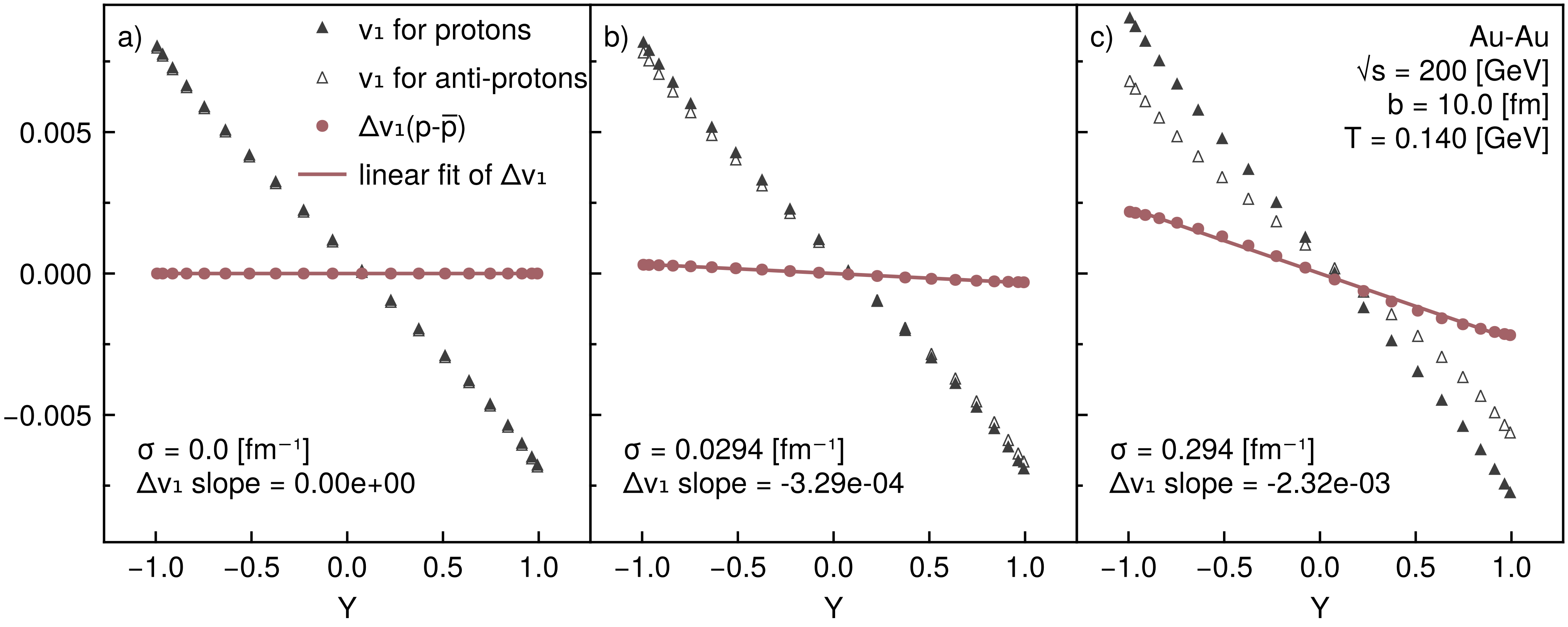
An observable difference between the charge of protons and anti-protons is illustrated in Fig. 5, where the conductivity of QGP is varied across the panels. The rapidity dependence of (anti-)proton charge dependent directed flow Eq.(20) separates in panels b and c. That separation is captured by a nonzero difference from Eq.(19). This is a similar result as the observations at the STAR experiment [16].
In panel a of Fig. 5 for zero conductivity, , the difference between flows is zero because we have assumed the initial charge density is in equilibrium, i.e., . This means the solution for Ohm’s law in Eq.(5) is always zero. By increasing the conductivity in panels b and c the proton and anti-proton directed flow separate. This is expected from ohm’s law Eq.(5) and our discussions about Figs. 3 and 4 that larger conductivities increase on the freezeout hypersurface, which results in more significant differences between the charged directed flow.
The negative linear slope of in panels b and c of Fig. 5 is a sign that the Faraday current has a greater net effect than the Lorentz current, which is in agreement with Ref. [15]. This shows the approximation of the Faraday current as and the Lorentz current as at the beginning of Sec. III holds for our RRMHD model. Moreover, an order increase in the electric conductivity brought a similar increase in the slope, suggesting this observable could be used to understand , the electric conductivity of QGP. Although, a more refined model is required to draw any quantitative conclusions.
VI.1 Centrality dependence of charge dependent flow
In our previous work [21], of pions were studied instead of protons. The result of that work proposed the electric conductivity of QGP should be or smaller when fit to experimental data. However, experimentally, the values of depend on the type of hadron (pions vs. protons) and the centrality of the collision [16, 18]. The centrality dependence occurs because the EM field intensity is proportional to the number of collision spectators, which means ultra-central collisions should have a smaller intensity than peripheral collisions. Then the decrease in EM intensity translates to smaller slopes of . This trend is reflected in the STAR data of for protons and anti-protons between and centrality [16].
Figure 6 illustrates that our RRMHD model can capture how smaller centralities translate into a smaller . The dependence on electrical conductivity changes non-trivially across centralities, with a conductivity similar to lattice having the least change over centralities [7]. In addition, the slope is always negative, which indicates the Faraday current always has a greater net effect than the Lorentz current in our model. However, as was discussed in Ref. [15], the initial protons in the collision mean the plasma would have a net positive charge. Until this point, we have considered the initial charge density to be zero, . The issue is initial dynamics of QGP have not been agreed upon, so a quantitative charge density distribution is difficult to establish. If we consider a phenomenological model like Ref. [37] for the baryon charge density and multiply it by the initial nuclei to calculate the electric charge density, we can get a rough idea of the initial electric charge density . See appendix A for a detailed discussion on the implementation.
For central collisions of fm, by choosing based on 197Au, we see an increase in ,
| (21) |
This demonstrates that an initial positive charge can result in positive slopes for with our RRMHD model. This result is dependent on how the initial charge density is defined and the conductivity of QGP. For example, the slope does not become positive for the largest conductivity value in Fig. 6 of ,
| (22) |

VII Conclusions
We have demonstrated how our relativistic resistive magneto-hydrodynamic (RRMHD) model can be used to study the charge dependent directed flow across collision centralities. The negative slope of was found to strongly depend on QGP’s electric conductivity, , which is a unique feature of our model. The slope of is caused by an electric charge imbalance on the freezeout hypersurface as illustrated in Figs. 3 and 4 in combination with the Cooper-Frye formula. This is the first work to establish such behavior and test is across centralities, which is shown in Fig. 6.
In future work, we aim to improve our model in several ways. Our results suggest that a complete modeling of requires a combination of baryon and electric charges. This means incorporating the Transported quark effects of Refs. [37, 38] with the electric conductivity effects of our RRMHD model. It is possible to accomplish that incorporation using a phenomenological approach as described in appendix A, or a more sophisticated model of the initial collision stages. Moreover, a dedicated analysis of how different models of the initial stages change the initial EM fields + charge density would be interesting on its own.
Another important improvement is the inclusion of vortical effects on the magnetic field. It has been established by experimental data with phenomenological models that collision participants and the resulting QGP have a large angular momentum. Theoretical models suggest that angular momentum could positively modify the time evolution of the magnetic fields. Incorporating that effect in our model should result in a better description of the electromagnetic fields.
The previous improvements focus on improving the accuracy of calculating the charge density . For a consistent calculation, we should use an equation of state (EoS) that includes the electric chemical potential, for example [39]. Although, considering in this work the charge density was found to be small on the freezeout hypersurface, the impact of changing the EoS to include the electric chemical potential may also be small.
In this work, we have assumed the electric conductivity of QGP is a scalar. But, dimensional analysis shows the conductivity should be temperature-dependent and dedicated calculations of the conductivity agree [7]. Additionally, for intense magnetic fields, the conductivity splits into a component parallel with the magnetic fields and a component perpendicular. Considering both of though effects would change the conductivity from a scalar to a tensor. A future investigation about how a tensor conductivity could affect experimental observables maybe interesting.
We have chosen a single freezeout temperature and then used the Cooper-Frye formula to calculate the final particle distributions. This is quite an oversimplification of the final hadron dynamics that would be better described with an afterburner + EM field calculation. Possible candidates are the kinetic solvers UrQMD, SMASH, or JAM, and ideally, we would like our model to be able to interface with all three.
Lastly, it has been well established that viscous hydrodynamics is required to explain the elliptical flow of final state hadrons. Although, it may seem natural to include viscosity in our model, because of how it could modify the Lorentz current, we do not believe it to be as important as other improvements. For example, our results agree with Ref. [15] even though they use iEBE-VISHNU + a perturbative EM field calculation.
Even without those changes, we have demonstrated a relationship between the negative slope of and QGP’s electric conductivity, in Figs. 5 and 6. This contrasts with other works [37, 38] that have focused on initial baryon charges and currents to explain the experimental data. In addition, we also demonstrated how initial positive charge can also cause positive slopes for , as was originally discussed in Ref. [15]. All of this work suggests an understanding of charge dependent directed flow at STAR [16] and ALICE [18] calls for a consideration of QGP’s electric conductivity.
Acknowledgements.
We thank Azumi Sakai for useful discussions and a thorough review of the initial manuscript. Furthermore, we thank Hidetoshi Taya and Akihiko Monnai for insightful discussions about early versions of this work. The numerical computation in this work was carried out at the Yukawa Institute Computer Facility. N.J.B. is grateful for the financial support from Hiroshima University’s presidential discretionary fund and Start-Up program fund. This work was also supported by JSPS KAKENHI Grant Numbers, JP20K11851, JP20H00156, JP24K07117 (T.M.), JP20H00156, JP20H11581 (C.N.), JP21H04488, JP24K00672, and JP24K00678 (H.R.T.). Perceptually uniform color maps are used in this study to prevent visual distortion of the data and to better serve those with color vision deficiency [40].Appendix A Effects from an initial charge density
We include a rough estimate of the initial charge density based on the phenomenological ansatz used to calculate and initial baryon number in Ref. [37]. This involves reusing the wounded nucleon’s weight profile of the tilted optical Glauber model. Because this is a rough estimate, we assume an initial charge density of,
| (23) |
The terms are the thickness functions of the individual nuclei shifted in the transverse plane by the impact parameter ,
| (24) |
where are the normalized nuclei Fermi distributions. We have used a radius of , a width of , and a nuclear saturation density of for 197Au. The functions in Eq.(23) impose a tilt in the longitudinal direction and define a longitudinal profile [31]. For the initial baryon number calculation in Ref. [37], an additional longitudinal weighting is preformed with that has two free parameters and . We ignore in this work because fixing those parameters requires solving the hydrodynamic evolution with a nonzero baryon current such that the ratio of transported and produced baryons at central rapidities can be reproduced. We do include a ratio parameter between the initial number of baryons vs. number of protons, which acts as a conversion from the initial baryon charge to the initial electric charge.
Appendix B Charge dependent freeze-out algorithm
We start from the usual Cooper-Frye formula,
| (25) |
and take the local thermal distribution,
| (26) |
where is the quantized electric charge of the hadron. For this work, we simplify the electric charge chemical potential to the linear approximation of the local charge density . This results in,
| (27) |
where is the hadronic degrees of freedom.
Appendix C Dependence on the intensity of the initial electromagnetic fields
We mentioned in Sec. III the pre-equilibrium dynamics after the collision could change the configuration of the initial EM fields. Results in Ref. [26], which uses a Kinetic model for the pre-equilibrium dynamics, suggests the EM fields decay like in a vacuum initially. The initial condition we used assumes the EM fields are in a conducting medium, thus the EM fields decay is that of in a medium [25]. After comparing the two methods at the initialization time of our simulation , we find a difference of approximately in the intensity of the magnetic field at the center of the grid.
We reproduce the panel of Fig. 5 after decreasing the intensity of initial EM fields by 0.1 across the entire computational domain. In Fig. 7, the slope of is reduced by an order of magnitude proportional to the same reduction of the initial EM fields from to . This suggests our results are equally sensitive to the electric conductivity of QGP and the initial EM fields.

References
- Jacak and Müller [2012] B. V. Jacak and B. Müller, The exploration of hot nuclear matter, Science 337, 310 (2012), https://www.science.org/doi/pdf/10.1126/science.1215901 .
- Bzdak and Skokov [2012] A. Bzdak and V. Skokov, Event-by-event fluctuations of magnetic and electric fields in heavy ion collisions, Physics Letters B 710, 171 (2012), arXiv:1111.1949 [hep-ph] .
- Deng and Huang [2012] W.-T. Deng and X.-G. Huang, Event-by-event generation of electromagnetic fields in heavy-ion collisions, Physical Review C 85, 044907 (2012), arXiv:1201.5108 [hep-ph] .
- Hattori and Satow [2016] K. Hattori and D. Satow, Electrical conductivity of quark-gluon plasma in strong magnetic fields, Physical Review D 94, 114032 (2016), arXiv:1610.06818 [hep-ph] .
- Li et al. [2018] W. Li, S. Lin, and J. Mei, Conductivities of magnetic quark-gluon plasma at strong coupling, Physical Review D 98, 114014 (2018), arXiv:1809.02178 [hep-th] .
- Astrakhantsev et al. [2020] N. Y. Astrakhantsev, V. V. Braguta, M. D’Elia, A. Y. Kotov, A. A. Nikolaev, and F. Sanfilippo, Lattice study of electromagnetic conductivity of quark-gluon plasma in external magnetic field, Physical Review D 102, 054516 (2020), arXiv:1910.08516 [hep-lat] .
- Aarts and Nikolaev [2021] G. Aarts and A. Nikolaev, Electrical conductivity of the quark-gluon plasma: perspective from lattice QCD, The European Physical Journal A 57, 118 (2021), arXiv:2008.12326 [hep-lat] .
- Ghosh and Shovkovy [2024] R. Ghosh and I. A. Shovkovy, Electrical conductivity of hot relativistic plasma in a strong magnetic field, Physical Review D 110, 096009 (2024), arXiv:2404.01388 [hep-ph] .
- [9] G. Almirante, N. Astrakhantsev, V. V. Braguta, M. D’Elia, L. Maio, M. Naviglio, F. Sanfilippo, and A. Trunin, Electrical conductivity of the quark-gluon plasma in the presence of strong magnetic fields, arXiv:2406.18504 [hep-lat] .
- Yin [2014] Y. Yin, Electrical conductivity of the quark-gluon plasma and soft photon spectrum in heavy-ion collisions, Physical Review C 90, 044903 (2014), arXiv:1312.4434 [nucl-th] .
- Rapp [2024] R. Rapp, Electric conductivity of qcd matter and dilepton spectra in heavy-ion collisions, Physical Review C 110, 054909 (2024), arXiv:2406.14656 [hep-ph] .
- Hirono et al. [2014] Y. Hirono, M. Hongo, and T. Hirano, Estimation of the electric conductivity of the quark gluon plasma via asymmetric heavy-ion collisions, Physical Review C 90, 021903 (2014), arXiv:1211.1114 [nucl-th] .
- STAR Collaboration [2017] STAR Collaboration, Charge-dependent directed flow in cu + au collisions at s n n = 200 gev, Physical Review Letters 118, 012301 (2017), arXiv:1608.04100 [nucl-ex] .
- Gürsoy et al. [2014] U. Gürsoy, D. Kharzeev, and K. Rajagopal, Magnetohydrodynamics, charged currents, and directed flow in heavy ion collisions, Physical Review C 89, 054905 (2014), arXiv:1401.3805 [hep-ph] .
- Gürsoy et al. [2018] U. Gürsoy, D. Kharzeev, E. Marcus, K. Rajagopal, and C. Shen, Charge-dependent flow induced by magnetic and electric fields in heavy ion collisions, Physical Review C 98, 055201 (2018), arXiv:1806.05288 [hep-ph] .
- STAR Collaboration [2024] STAR Collaboration, Observation of the electromagnetic field effect via charge-dependent directed flow in heavy-ion collisions at the relativistic heavy ion collider, Physical Review X 14, 011028 (2024), arXiv:2304.03430 [hep-ph] .
- STAR Collaboration [2014] STAR Collaboration, Beam-energy dependence of the directed flow of protons, antiprotons, and pions in au+au collisions, Physical Review Letters 112, 162301 (2014), arXiv:1401.3043 [nucl-ex] .
- A Large Ion Collider Experiment Collaboration(2020) [ALICE] A Large Ion Collider Experiment (ALICE) Collaboration, Probing the Effects of Strong Electromagnetic Fields with Charge-Dependent Directed Flow in Pb-Pb Collisions at the LHC, Physical Review Letters 125, 022301 (2020), arXiv:1910.14406 [nucl-ex] .
- Inghirami et al. [2016] G. Inghirami, L. Del Zanna, A. Beraudo, M. H. Moghaddam, F. Becattini, and M. Bleicher, Numerical magneto-hydrodynamics for relativistic nuclear collisions, The European Physical Journal C 76, 659 (2016), arXiv:1609.03042 [hep-ph] .
- Inghirami et al. [2020] G. Inghirami, M. Mace, Y. Hirono, L. Del Zanna, D. E. Kharzeev, and M. Bleicher, Magnetic fields in heavy ion collisions: flow and charge transport, The European Physical Journal C 80, 293 (2020), arXiv:1908.07605 [hep-ph] .
- Nakamura et al. [2023a] K. Nakamura, T. Miyoshi, C. Nonaka, and H. R. Takahashi, Charge-dependent anisotropic flow in high-energy heavy-ion collisions from a relativistic resistive magneto-hydrodynamic expansion, Physical Review C 107, 034912 (2023a), arXiv:2212.02124 [hep-ph] .
- Nakamura et al. [2023b] K. Nakamura, T. Miyoshi, C. Nonaka, and H. R. Takahashi, Relativistic resistive magneto-hydrodynamics code for high-energy heavy-ion collisions, The European Physical Journal C 83, 229 (2023b), arXiv:2211.02310 [nucl-th] .
- Nakamura et al. [2023c] K. Nakamura, T. Miyoshi, C. Nonaka, and H. R. Takahashi, Directed flow in relativistic resistive magneto-hydrodynamic expansion for symmetric and asymmetric collision systems, Physical Review C 107, 014901 (2023c), arXiv:2209.00323 [nucl-th] .
- Tuchin [2016] K. Tuchin, Initial value problem for magnetic fields in heavy ion collisions, Physical Review C 93, 014905 (2016), arXiv:1508.06925 [hep-ph] .
- Tuchin [2013] K. Tuchin, Time and space dependence of the electromagnetic field in relativistic heavy-ion collisions, Physical Review C 88, 024911 (2013), arXiv:1305.5806 [hep-ph] .
- Yan and Huang [2023] L. Yan and X.-G. Huang, Dynamical evolution of a magnetic field in the preequilibrium quark-gluon plasma, Physical Review D 107, 094028 (2023), arXiv:2104.00831 [nucl-th] .
- McLerran and Skokov [2014] L. McLerran and V. Skokov, Comments about the electromagnetic field in heavy-ion collisions, Nuclear Physics A 929, 184 (2014), arXiv:1305.0774 [hep-ph] .
- Matsuda and Huang [2024] H. Matsuda and X.-G. Huang, Simulation of a (3+1)D glasma in Milne coordinates: Topological charge, eccentricity, and angular momentum, Physical Review D 110, 114032 (2024), arXiv:2409.08742 [hep-ph] .
- Li et al. [2023] H. Li, X.-L. Xia, X.-G. Huang, and H. Z. Huang, Dynamic calculations of magnetic field and implications on spin polarization and spin alignment in heavy ion collisions, Phys. Rev. C 108, 044902 (2023), arXiv:2306.02829 [nucl-th] .
- Dash and Panda [2024] A. Dash and A. K. Panda, Charged participants and their electromagnetic fields in an expanding fluid, Physics Letters B 848, 138342 (2024), arXiv:2304.12977 [hep-th] .
- Bożek and Wyskiel [2010] P. Bożek and I. Wyskiel, Directed flow in ultrarelativistic heavy-ion collisions, Physical Review C 81, 054902 (2010).
- d’Enterria and Loizides [2021] D. d’Enterria and C. Loizides, Progress in the glauber model at collider energies, Annual Review of Nuclear and Particle Science 71, 315 (2021), arXiv:2011.14909 [hep-ph] .
- Cooper and Frye [1974] F. Cooper and G. Frye, Comment on the single particle distribution in the hydrodynamic and statistical thermodynamic models of multiparticle production, Physical Review D 10, 186 (1974).
- Huovinen and Petersen [2012] P. Huovinen and H. Petersen, Particlization in hybrid models, The European Physical Journal A 48, 171 (2012), arXiv:1206.3371 [hep-ph] .
- Mattia et al. [2023] G. Mattia, L. Del Zanna, M. Bugli, A. Pavan, R. Ciolfi, G. Bodo, and A. Mignone, Resistive relativistic MHD simulations of astrophysical jets, Astronomy & Astrophysics 679, A49 (2023), arXiv:2308.09477 [astro-ph] .
- Shen et al. [2016] C. Shen, Z. Qiu, H. Song, J. Bernhard, S. Bass, and U. Heinz, The iEBE-VISHNU code package for relativistic heavy-ion collisions, Computer Physics Communications 199, 61 (2016), arXiv:1409.8164 [nucl-th] .
- Bożek [2022] P. Bożek, Splitting of proton-antiproton directed flow in relativistic heavy-ion collisions, Physical Review C 106, L061901 (2022), arXiv:2207.04927 [nucl-th] .
- Guo et al. [2012] Y. Guo, F. Liu, and A. Tang, Directed flow of transported and nontransported protons in Au + Au collisions from an ultrarelativistic quantum molecular dynamics model, Physical Review C 86, 044901 (2012), arXiv:1206.2246 [nucl-ex] .
- Monnai et al. [2024] A. Monnai, G. Pihan, B. Schenke, and C. Shen, Four-dimensional QCD equation of state with multiple chemical potentials, Physical Review C 110, 044905 (2024), arXiv:2406.11610 [nucl-th] .
- Crameri et al. [2020] F. Crameri, G. E. Shephard, and P. J. Heron, The misuse of colour in science communication, Nature Communications 11, 5444 (2020).